Sage Journals: Discover world-class research

Abstract

To overcome the limitations of traditional data collection methods in large-scale farmland wireless sensor network, in this study, we introduce a mobile sink and propose a virtual potential field-based strategy for mobile sink path planning. Virtual potential field-based strategy constructs a virtual field based on the residual energy, data generation rate, location information and cache urgency of nodes in the monitoring area. The stronger the virtual field, the more attractive it will be to mobile sink, which consequently affects the mobile path of sink node. Rendezvous points are selected in accordance with the maximum-farthest criterion, and the shortest path connecting all rendezvous points is taken as the mobile path of sink. Furthermore, the monitoring nodes employ the distance probability transmission strategy to have the transmission moment selected and the energy consumption optimized with reference to the path control information sent by the sink. The virtual potential fields and the rendezvous points are recalculated periodically according to the dynamic changes of both the node residual energy and the real-time cache. The simulation results showed that excellent transmission efficiency and network lifetime, and the combination of virtual potential field-based strategy and distance probability transmission strategy can have the fairness and real time of nodes guaranteed, thus it may meet the needs of large-scale farmland data collection.

Keywords

Farmland wireless sensor networks mobile sink path planning network lifetime energy efficiency wireless sensor network transmission strategy

Introduction

As the link between the physical world and the information world, wireless sensor networks (WSNs) may realize the digitization of analog data, thus greatly increases the range and accuracy of cognitive ability of human beings, that is why it has been widely used in industries, agriculture, medical treatment, military and other fields. The energy management and resource allocation^1,2 of WSN run through almost all aspects of WSN research, no doubt they are of significance to WSN application. In many researches, a lot of work has been done in terms of energy management, routing strategy³ and load balance. Concepts like mobile sink, intelligent reflector and rechargeable nodes⁴ have been introduced, which provide us with many solutions for optimizing the WSN energy consumption management.

These key issues are also important in agriculture application. The intelligent management of large-scale farmland WSN is crucial for the advancement of agricultural production. Accurate environmental and crop data are essential for the accurate application of the Agricultural Internet of things (IOT) and precision agriculture.

With farmland monitoring areas expanding, the limitations of traditional data collection methods have become more and more evident. For example, multi-hop or cluster-based routing is prone to hot spots,⁵ energy holes and related problems caused by uneven energy consumption. The introduction of mobile sink^2,3 greatly alleviates the problems as mentioned above, though the path planning of mobile sink and data transmission of nodes are still facing great challenge, which restricts the performance of farmland WSNs. Moreover, due to large variations in the types and quantities of monitoring data, efficient collection methods that are suitable for large-scale heterogeneous farmland are still in great needs at present.

There are several key problems for mobile path planning in large-scale farmland monitoring scenarios: first, large monitoring areas make it difficult to guarantee the fair access of each node. For the same reason, it is hard to ensure the timeliness and validity characteristics of data. In addition, low redundancy of node deployment may cause large node spacing, which makes frequent multi-hop transmission costly. What’s more, the heterogeneity of nodes and data makes the transmission load uneven.

The scope of the article is to determine a move strategy for mobile sink before having the transmission strategy of data designed.

In the current study, we aim to (1) improve data collection efficiency and extend the lifetime of farmland WSNs; (2) meet the real-time data collection requirements of large-scale farmland WSNs; (3) avoid the imbalance of node energy consumption and the unfairness of sink access; and (4) reduce the network maintenance costs. To achieve these objectives, a virtual potential field for large-scale farmland monitoring networks was built, and a mobile sink path as well as a data collection strategy suitable for farmland data characteristics is designed.

The main contributions in this article include the following aspects. First, we build a virtual potential field to reflect the state of the nodes in WSNs; second, we propose a method to select rendezvous points (RPs) from the virtual potential field; third, we recalculate RPs periodically to adapt the dynamic changes of nodes. Finally, distance probability transmission strategy minimizes transmission energy consumption. Quantities of simulations prove the efficiency of our presented method in aspects of balance of energy consumption, network lifetime and the efficiency of data gathering.

The rest of this article is organized as follows. A brief summary of some latest research achievement is given in section ‘Related work’. In section ‘Scenario assumptions and parameter descriptions’, the scenario assumptions and parameter descriptions are illustrated. In section ‘Behaviour strategy of nodes in large-scale farmland WSNs’, our algorithm is described in detail. In section ‘Simulation and results’, simulations are conducted and the results are analysed. Finally, we conclude the whole article in section ‘Conclusion’.

Related work

During the monitoring of a WSN with a mobile sink, it is found that the data collection efficiency of the WSN is significantly affected by the mobile mode of the sink. This issue has been the focus of many researches, and extensive progress has been made on it. The principle moving modes of the mobile sink are fixed paths,^6,7 random paths⁸ (including random movement under certain constraints), autonomous moving^9–11 and rendezvous-based paths.¹²

The fixed path refers to the reciprocating movement along pre-designed paths such as straight lines¹³ and loops. The movement without path calculations is simple to operate; however, due to its poor flexibility, this mode has a limited effect on the lifetime extension of the network. In Chhieng et al.,¹⁴ the network area is subtly divided and the space filling curve is employed to design the mobile route. By adjusting the granularity of the path according to the actual needs, the path ensures the fairness of the network. However, this moving method requires frequent turns, and the granularity cannot be changed continuously, thus it is still difficult to meet the challenge of changing network environment.

Random movement allows the sink to move randomly in the monitoring area, or allow sink to randomly decide the next moving direction under certain constraints. The flexibility of this type of algorithm is greater than that of the fixed path, yet generating to the situation that the real-time state of the network can be complicated and the fairness of data transmission cannot be guaranteed.

Autonomous moving denotes the ability of the mobile sink to choose and adjust its own motion state according to the needs of the network. Generally, the algorithm drives the mobile sink to move to nodes with higher residual energy or areas with a high node density or transmission requirements. This avoids congestion and network hot areas. In Bi et al.,⁹ the sink is moved to nodes with high residual energy, while nodes with low residual energy are avoided in order to alleviate the energy consumption imbalance resulting from data forwarding in multi-hop transmission scenarios. In Reiser et al.,¹⁵ a four-wheel robot is employed as a mobile sink to locate all nodes follow a predefined way-point path, thus an appropriate autonomous path is generated according to node locations as well as their received signal strength indication (RSSI) collected from the predefined path.

Rendezvous-based paths select appropriate RPs in the monitoring area and subsequently plan the shortest path to connect the RPs. Optimization objectives (reducing data delivery delays, shortening mobile path and extending the network lifetime) can vary with selection method. For example, in Cheng and Yu,¹⁶ the mobile sink accesses the overlapping area of the sensor communication range in a proper sequence, instead of the location of the sensor itself, and the travelling salesman problem (TSP) algorithm is applied to obtain the path. This type of algorithm often employs node clustering and allows mobile sink access cluster heads to shorten the mobile distance, which may reduce the delivery delay and energy consumption and improve the network lifetime. The authors of Nguyen et al.¹² combine two methods, the cluster-head election algorithm and the mobile sink trajectory optimization algorithm, to propose the optimal movement strategy. The strategy minimizes both the energy consumption and data gathering periods and achieves both a long network lifetime and an optimal mobile sink schedule. In Chu and Ssu,¹⁷ a cluster-based mobile sink exploration (CMSE) scheme is developed to guide data packets efficiently to mobile sinks and multiple routing paths are established from a sensor to the sink to enhance network longevity.

Recently, the rise of articles-machine learning algorithms provides many optimization schemes for WSN data collection and path determination. In Wang et al.,¹⁸ an improved particle swarm optimization combined with mutation operator is introduced to search the parking positions and the genetic algorithm is adopted to schedule the moving trajectory for mobile sinks. Donta et al.¹⁹ propose an extended ant colony optimization-based mobile sink path construction, with RPs re-selection and virtual RPs to improve WSNs’ performance. The unsupervised learning-based hierarchical agglomerative clustering method is used in Donta et al.²⁰ to solve the problem in three-dimensional (3D) WSNs with mobile sink. These algorithms usually need a certain amount of training samples to ensure the effectiveness of the model. So, we try to use less prior knowledge to build a more concise model.

With respect to the data transmission of a mobile sink–integrated WSN, the majority of research focuses on balancing the energy consumption of nodes and prolonging the life span of the network through reasonable routing, clustering and cluster head election methods. In Sha et al.,²¹ network is divided into several virtual regions and one or more leaders are selected in each region according to their residual energy, which reduces the cost of cluster head election and rotation, at the same time balances the energy consumption of the whole network. In Nguyen et al.¹² and Liu et al.,²² the priority or transmission power (radius) of nodes is assigned to different energy states in order to balance the energy consumption of the nodes. Kostin et al.²³ employ a routing scheme based on expanding ring search and anycast messaging. The scheme randomly selects smaller broadcasting propagation distances in different propagation directions, thus avoiding the excessive energy consumption of nodes and network traffic. Several performance metrics are also investigated to test the effectiveness of the scheme. In Wang et al.,²⁴ nodes are cleverly clustered and energy consumption of different routing paths are skilfully calculated to choose the optimal scenario. CHs are connected into a chain using the greedy algorithm to enhance network performance. In the delay-tolerant WSN^25–27 framework, a time interval is specified between the generation and collection of data. In practical applications, it is also necessary to formulate data transmission strategies according to the specific needs of the network. For example, Li et al.²⁵ proposed a novel social-based routing approach for mobile social delay-tolerant networks. Social energy is generated via node encounters and shared by the communities of encountering nodes, which quantify the ability of a node to forward packets to others. In Jacquet et al.,²⁶ analytical tools are used to derive generic theoretical upper bounds for the information propagation speed in large-scale mobile and intermittently connected networks.

Each of the sink mobility strategies and transmission rules can improve the transmission performance of the WSN; however, each method has its own limitations. Fixed paths and paths based on fixed RPs are easy to implement, yet their overall flexibility is poor, and it is difficult for them to adapt to the dynamic topology changes caused by network node failure and death. Although random paths are flexible, they are unable to meet the real-time requirements of the network effectively. While the autonomous path selection method is able to respond to network changes, yet it cannot guarantee the fairness of the nodes. This may prevent sink access to nodes for an extended period of time. RP-based path performance is closely related to the RP selection strategy. In order to fulfil the node transmission requirements and to account for the access flexibility and network fairness, in this study, a dynamic RP selection criterion based on node status is developed to improve the data collection performance of farmland WSNs by continuously rotating the RPs.

Scenario assumptions and parameter descriptions

Basic network hypothesis

Based on the need for cost efficiency and data accuracy, large-scale farmland WSNs exhibit the following characteristics: large monitoring area, node sparseness, and complex node compositions and data types. Therefore, the energy consumption of a single transmission is high and unbalanced. It is necessary to balance the energy consumption of each node to avoid rapid death, which consequently results in data and energy voids.

We made the following assumptions based on the above characteristics:

N sensor nodes denoted by {node₁, node₂ …, node_N} are randomly and evenly deployed in square farmland areas of $W \times W$ .

The ith sensor node has initial energy E_0i and produces a L_0i-length packet. Its status is expressed as {(x_i, y_i), [E_i, E_0i], [l_i, L_0i]} which represent {(coordinate position), [residual energy, initial energy], [current buffer length, data generation rate]}.

The speed of mobile sink (MS) is v, and the endurance time of MS carrier is $T_{r_\max}$ .

The motion height of MS and Doppler effect on data transmission are not considered. Transmission times, data collision and retransmit between nodes are also ignored.

In the MS-integrated WSN, the periodic movement of MS in the monitoring area is known as a ‘round’. $Δ T (Δ T > T_{r_\max})$ is denoted as the single-round interval of the network. The MS begins a new network information collection round in integral times of $Δ T$ and all nodes produce a packet waiting to be transmitted.

Data transmission characteristics and energy consumption model

The farmland WSN is a typical monitoring delay-tolerant WSN that allows a network in which nodes do not have to send data immediately when it is received, rather they can temporarily cache it and send it at the appropriate time. Therefore, delay insensitivity can be used for network energy consumption optimization, in avoiding frequent data transmission and continuous channel listening, thus node energy can be saved to increase the lifetime of the network.

However, due to the node sparseness in farmland WSNs, the channel between nodes can be obscured by crops, thus increasing the transmission cost between nodes. Therefore, the massage transmission between nodes must be reduced to avoid excessive energy consumption.

The energy consumption required by the nodes in the WSN to send and receive messages can be described by equations (1) and (2),^12,28 where $E_{re}$ and $E$ are the energy consumption required by the nodes for receiving and sending messages, respectively; $E_{clc}$ , $ε_{fs}$ and $ε_{mp}$ are constants that represent the circuit energy consumption factor, free space path loss factor and multipath loss factor, respectively; l is the length of the data packet. d is the distance between source and destination nodes; k is the path loss factor determined by the environment, generally between 2 and 6; d₀ is the threshold that distinguishes free paths from multipath paths, as shown in equation (3)

E_{re} = l \times E_{clc}

(1)

Etr = {\begin{matrix} l (E_{clc} + ε_{fs} d^{k}) & d \leq d_{0}, k = 2 \\ l (E_{clc} + ε_{mp} d^{k}) & d > d_{0}, k = 4 \end{matrix}

(2)

d_{0} = \sqrt{\frac{ε_{fs}}{ε_{mp}}}

(3)

When the transmission distance is less than or equal to d₀, the channel is considered to be a free space path with a path loss factor of $ε_{fs}$ and the value of k is 2. While for transmission distances greater than d₀, the channel is considered to be a multipath path with a path loss factor $ε_{mp}$ , with k is equal to 4.

Network lifetime and energy balance index

In practical WSN applications, the network is expected to function as long as possible after deployment. The lifetime of a WSN usually refers to the time interval T from the start of the WSN operation up until the WSN is unable to function properly due to the energy exhaustion of the nodes. Lifetime T is an important measure of WSN performance. In the MS-integrated WSN, the number of rounds (ROUNDs) is often used as a measure of WSN lifetime. In the current study, the relationship between T and ROUNDs is as follows

T = Δ T \times ROUNDs

(4)

The farmland WSN monitoring process is associated with a redundancy in node deployment. More specifically, when the proportion of dead nodes increases to a certain value, the network cannot function properly because of the energy and information holes, which result in network failure.

The energy of the nodes in the WSN is gradually consumed as the network runs. Thus, we aim to keep as many surviving nodes as possible during the WSN operation, namely, the lifetime of all nodes should be as approximate as possible.

In order to measure the energy balance of the nodes in the WSN, we define the energy balance index (EBI) of the network is defined as follows, where R_x denotes the number of rounds as x% of the nodes die

EBI = \frac{R_{50}}{R_{90} - R_{10}}

(5)

EBI represents the ratio of R₅₀ (WSN lifetime) to the difference in the number of rounds from 10% to 90% of node deaths. The larger the EBI value, the better the energy consumption balance of the nodes. To raise the EBI not only increases the stability of WSN performance, but also helps to prolong its lifetime.

In summary, under the aforementioned network assumptions and scenarios, the aim of the current study is to design an effective sink mobile path that cooperates with the node routing strategy, reduces the energy consumption of nodes, and improves the network lifetime and energy balance to meet the needs of large-scale farmland WSN applications.

Behaviour strategy of nodes in large-scale farmland WSNs

VPFBS: virtual potential field-based strategy for mobile sink path planning

In large-scale farmland WSNs with a mobile sink, the mobile strategy of the MS and the message transmission strategy of the nodes form the most crucial components of the network. Here, we have a discussion of the path planning of the MS.

Mobile sink path planning process

For an efficient MS path, not only the energy consumption balance and fair transmission of nodes but also the limitation of the actual movement ability of mobile carriers (e.g. endurance time and mobile speed) needs to be considered. Furthermore, in order to minimize unnecessary data transmission and channel listening, nodes require a priori knowledge of the MS movement track to reduce the frequent transmission of control information. The nodes must also remain dormant during the non-data transmission stage to avoid excessive energy consumption and prolong the lifetime of the network.

An MS path planning scheme is proposed based on a virtual potential field that is suitable for large-scale farmland WSN with mixed heterogeneous nodes (i.e. nodes in the network have different functions, data generation rates, initial energy). By calculating the virtual potential field in the entire monitoring network area, the selected RP locations can simultaneously accommodate the complex combinations of different deployment and functions of nodes and balance the energy consumption. The virtual potential fields and RPs are recalculated periodically to adapt to the real-time changes of the network.

Figure 1 depicts an example of the MS movement in the monitoring area. In Figure 1(a) nodes are randomly distributed. The virtual potential field is calculated as shown in Figure 1(b). Then, five RPs are selected through the virtual potential field at the current moment (Figure 1(c)). Finally, Figure 1(d) shows that the MS accesses each RP sequentially along the shortest path, and the monitoring nodes send messages at the closest location to the MS. In the next round, the calculation of potential field (b), selection of RPs (c) and traversal of RPs (d) are repeated.

Figure 1.

Path planning steps for mobile sink: (a) node distribution, (b) virtual field calculation, (c) path planning and (d) RP selection.

After network initialization, the operation process of the MS is described as follows:

The MS calculates the virtual potential field P at all sampling points in the monitoring area based on the location of the nodes, the remaining energy, the rate of data generation and the urgency of the node cache (Part B).

The peak of the virtual potential field P obtained in step 1 is used as the candidate point for the RP. The number of RPs (NR) is determined according to the actual requirements of the constraints and the RPs are selected from the candidate points as described in Part C.

The shortest path connecting the RPs is used as the moving path, where the MS accesses all RPs one by one at a uniform speed and collects node messages during the moving process. In each round, the MS continuously records the real-time energy and cache status of each node while collecting information. This information is used to calculate the real-time virtual potential field and also broadcasts control instructions to inform nodes of the next round motion track and wake-up control information.

The MS recalculates the virtual potential field, RP and moving path after each round based on the current node states. It then moves to the initial RP of the next round and waits for the next traversal.

The process is repeated until the network fails.

Once the behaviour of the MS is determined, the monitoring nodes will send the collected information to the MS via the transmission strategy as described in section ‘DPTS: distance probability transmission strategy for monitoring nodes’.

Construction of virtual potential field based on multi-factor node states

As described in Part A, as a characterization of the information transfer requirements in the monitoring area, the virtual potential field directly affects the selection of the RPs and the sink path. Here, we define and calculate the virtual potential field at any point in the monitoring area based on the distribution and current status (data generation rate, remaining energy, data cache) of the nodes.

Considering the data transfer requirements and the limitation of the sink movement resulting from environmental obstacles or boundaries, the virtual potential field in the network area is defined as the sum of the attraction potential field generated by the nodes and the exclusion potential field generated by the boundaries and obstacles.

Attractive potential field from nodes

The virtual potential field generated by a single sensor node i at any point in monitoring area is defined as

P_{node (i)} = P (Esr, L, dis, ITU) = P (Esr) P (L) P (dis) P (ITU)

(6)

Namely, the virtual potential field generated by node i is defined by the product of four components related to the remaining energy: P(Esr), the data generation rate: P(L), the impact range: P(dis), and the cached data urgency of node i: P(ITU). We then define virtual potential field component related to the residual energy of node i, as equation (7), where $P (Esr)$ is the component of the virtual potential field that is related to the residual energy of node i. Esr_i and Er represent the relative residual energy of node i and the average relative residual energy of all nodes, respectively

P (Esr) = \frac{Er - Es r_{i}}{Er} + 1

(7)

When the residual energy of node i is low, its attraction to MS increases, which subsequently drives the MS closer to the node, prevents the node from generating excessive energy consumption due to a long transmission distance and improves the energy balance of the network. Assuming that P(L) denotes the component related to the node data generation rate, then we get

P (L) = \frac{L_{i}}{\bar{L}}

(8)

where L_i and $\bar{L}$ denote the data generation rate for node i and the average data generation rates for all nodes, respectively. Due to the heterogeneity of the nodes, L_i may vary greatly. The introduction of P(L) can avoid the premature death of high data rate nodes, which will be more attractive to MS. We then define P(d) as the component that limits the influence range of the virtual potential field produced by a single node

P (dis) = {\begin{matrix} (e^{- \frac{dis}{d_{0}}} - e^{- 1}) & dis \leq d_{th} \\ 0 & dis > d_{th} \end{matrix}

(9)

where dis is the distance between the sample point and node i; d_th is the threshold of the influence range of a node. It is assumed that a single node can generate a virtual potential field within the radius of d_th centred at its own location that decreases with distance. In practical applications, d_th can be set based on the spatial accuracy of data. In the current study, we set d_th = d₀. In order to represent the latency urgency of node cached messages and to allow the data in the cache to be transmitted without long breaks, P(ITU) is defined as the information time urgency component

P (ITU) = α \frac{l_{i}}{\bar{L}}

(10)

where l_i is the current cache size of node i; $α$ is the information time emergency factor. Here, we take $α = R' - R + 1$ , where the earliest packet in the cache of node i is generated in round R and the current round is round R′. P(ITU) increases as the packet waiting rounds(R′–R) increase, which provides sufficient attraction for the MS. Furthermore, for an equal number of waiting rounds, nodes with more caches will generate larger P(ITU) values, which can take the real-time and fairness of network data transmission into account.

The virtual potential field generated by a node in a flat area is determined by the node’s current remaining energy, data generation rate, geographic location and the urgency of the cached data. The virtual potential fields of the entire monitoring area can be obtained by overlaying the virtual potential fields produced by each of the WSN nodes. Figure 2 presents the virtual potential field generated by 10 nodes with randomly distributed states and locations in a planar 1000 m × 1000 m monitoring area, with a spatial sampling interval of 10 m. The x-axis and y-axis represent the number of sample points in two directions on the plane, while the z-axis is the virtual potential field value corresponding to each sample point. Each node produces a potential peak at its corresponding location, whereby the size of the peak is positively related to its relative residual energy, data generation rate and information time emergency.

Figure 2.

Virtual potential field generated by nodes.

Repulsion of potential field from edge

The efficiency of the message transmission may be reduced for short distances between the MS and the monitoring area edge or obstacle. Thus, the MS path should be located far away from the both edge and the obstacle. For a square monitoring area whose vertex coordinates are (0, 0) (0, m) (m, 0) and (m, m), we define the negative boundary potential field P_edge as follows

P_{edge} = P_{edge} (x, y) = β \sum_{j = 1}^{4} P e_{j}

(11)

Note that no other obstacles are considered and the monitoring area boundary produces a constant rejection potential field for the MS. The value of P_edge decreases as the location moves away from the boundary. In equation (11), $β$ denotes the boundary potential field factor, with $β < 0$ . If each boundary is defined to have an impact range of d₀, the potential fields generated by the four boundaries are described as follows

\begin{matrix} P e_{1} = {\begin{matrix} \frac{1}{y} & y \leq d_{0} \\ 0 & y > d_{0} \end{matrix} P e_{2} = {\begin{matrix} \frac{1}{x} & x \leq d_{0} \\ 0 & x > d_{0} \end{matrix} \\ P e_{3} = {\begin{matrix} \frac{1}{m - y} & m - y \leq d_{0} \\ 0 & m - y > d_{0} \end{matrix} P e_{4} = {\begin{matrix} \frac{1}{m - x} & m - x \leq d_{0} \\ 0 & m - x > d_{0} \end{matrix} \end{matrix}

(12)

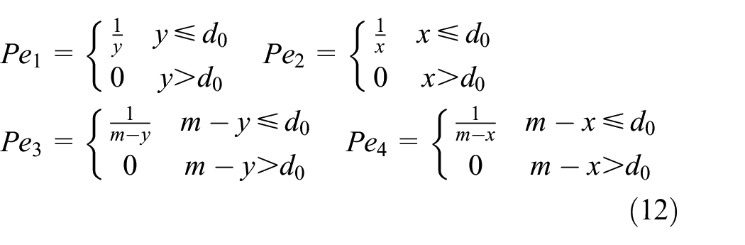
Figure 3 presents an example of a boundary potential field with a 1 km × 1 km monitoring area and a sampling interval of 10 m.

Figure 3.

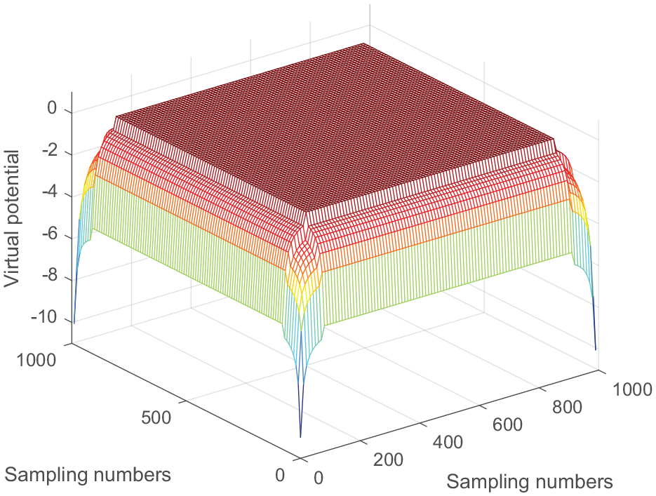
Virtual potential field generated by region boundaries.

Following equations (6) and (11), the virtual potential field can be obtained by overlaying the node potential field and the edge potential field of the monitoring area

P = P_{node} + P_{edge} = \sum_{i = 1}^{N} P_{node (i)} + β \sum_{j = 1}^{4} P e_{j}

(13)

where N represents the total number of nodes in the network, and P_node and P_edge are the virtual potential fields generated by all nodes and the region boundary (or barrier), respectively.

For the real scenario with a large number of nodes, the virtual potential fields produced by each node overlap each other. This can statistically reflect the attraction to the MS. Regions with a higher virtual potential field contain a greater amount of data to be transmitted and generally have a higher node density. Preferential access to these areas can increase the fairness of the data transmission.

In Northeast and North China, to improve the level of mechanization, farmland tends to have an area greater than 1000 acres in order. Thus, in the current study, we set the farmland area to be a square with a side length of 1000 m. Figure 4 presents a 3D diagram of a virtual potential field with 1000 nodes randomly distributed in a square monitoring area with a side length of 1000 m as well as a projection of the virtual potential field and node deployment in the monitoring plane.

Figure 4.

Virtual potential field and its corresponding node distribution: (a) 3D graph of virtual potential and (b) projection of virtual potential.

For areas with a dense node distribution, the virtual potential field is larger, and the probability of the MS approaching these areas is also greater, which is conducive to the efficient transmission of node information. Due to limitations in the communication range and energy, it is difficult for nodes to obtain the complete real-time status of other nodes in the whole network. The MS is able to track the status of each node while moving and collecting data and can maintain the ‘node status list’ that stores the latest information of all nodes. This information is subsequently used to plan the path and send control messages to each node.

Selection and rotation of RPs

During the network operation, the energy consumption and cache state of the nodes are constantly changing. The MS must adjust its own path to adapt to the new network state and optimize the energy consumption of the nodes. As detailed in Part A, the TPS path connecting all RPs is taken as the moving track of the MS. Thus, to optimize the MS trajectory, the optimal number and location of the RPs need to be determined.

Constraints on the number of RPs

The number of RPs (NR) strongly affects the network performance.^29,30 Statistically, the moving distance of the MS in each round increases with the number of RPs, while the average distance between the nodes and MS paths decreases. The smaller transmission distance and lower node energy consumption extend the life cycle of the network. Furthermore, NR is limited by the MS maximum working time $T_{r_\max}$ and the network single-round interval $Δ T$ . The length of each movement path, D_r, needs to be met

{\begin{matrix} D_{r} < T_{r_\max} \times v = D_{r_\max} \\ D_{r} < Δ T \times v \end{matrix}

(14)

For a constant NR, the path length D_r varies greatly with RP location. In this scenario, due to $T_{r_\max} < Δ T$ , D_r does not exceed the maximum distance of a single round.

To determine the limit for NR as well as the relationship between NR and the length of a single-round path, we perform 100 sets of simulations for each NR. The maximum of 100 sets of simulated path distances are selected, and a 10% margin is set as the NR selection limit to ensure that the MS traverses all the RPs in a single movement. More specifically, the longest path threshold is equal to the longest simulated path multiplied by 1.1. Section ‘Simulation and Results’ provides more details on the relationship between NR and the maximum path length.

In practical applications, an appropriate NR must be selected based on MS mobility, latency requirements and network lifespan.

Selection of RP location

Once the virtual potential field and the number of RPs have been determined, the RPs are selected to determine the moving path of the MS. Initially, the entire monitoring area is divided into girds according to the appropriate granularity, and the virtual potential field is then sampled at the cross points to obtain the distribution of the virtual potential field in the monitoring area. A larger virtual potential field indicates more data and a greater information density close to the location, which needs MS to access preferentially. Following this, the maximum points are selected as the candidate RP positions and are placed in the PEAKs set. Due to the large network area, the complex node distribution and the large number of elements in PEAKs, not all of points can be selected as RPs, that is why filtering is required. Assuming that the number of RPs required is NR (NR < crad (PEAKs)), the RP selection process is described as follows:

1. Initialize the empty RPs set to store the selected RPs, take the point with the largest virtual potential field value from the PEAKs set and move it into the RPs set as the initial RP.

2. The three points a, b and c with the highest virtual potential field values in PEAKs are used as candidate RPs. The sum of the distances from these three points to each point in the RPs set is calculated separately. For a given point in time, if the elements in two sets are shown in Figure 5, then calculate D_a, D_b and D_c

\begin{matrix} D_{a} = \sum_{i = 1}^{p} D (a, RPi) \\ D_{b} = \sum_{i = 1}^{p} D (b, RPi) \\ D_{c} = \sum_{i = 1}^{p} D (c, RPi) \end{matrix}

(15)

where D (a, RP_i) represents the distance between points a and RP_i.

3. Add the point corresponding to the maximum values of D_a, D_b, D_c as a new RP to the RPs set, and delete the point from the PEAKs set. This ensures that the newly selected RP is as far away as possible from the existing RPs while a high potential field value is guaranteed. Thus, the concentration of RPs in certain areas is avoided, allowing for the fairness of transmission. This selection strategy is denoted as the ‘maximum-farthest’ strategy.

4. Return to step 2 until the number of points in the RPs reaches the preset number NR.

Figure 5.

Changes in RPs and PEAKs during the RP selection.

The RPs are obtained and the shortest path through these points can be calculated. The MS moves along this path, collecting monitoring data and update the node status list.

RP rotation

The virtual potential field changes constantly while the network runs, preventing the original path from achieving the optimal effect. Therefore, the MS needs to calculate a new path based on the real-time states of the nodes following each collection round and notifies all nodes in the next round. The MS runs until the network fails. Table 1 details the path used in each round and the behaviour of the MS, and Figure 6 presents the flow of the MS.

Table 1.

MS path control.

Round	Round 1	Round 2	Round 3	…	Round r
Path used in current round	Initial path	Initial path	Path 1	…	Path r-2
Control information for current round	-	Inform nodes Path 1	Inform nodes Path 2	…	Inform nodes Path r-1
Work done by MS following current round	Real-time network status ↓ Virtual field $\begin{matrix} Calculate RP \\ ↓ \end{matrix}$ Path 1	Real-time network status ↓ Virtual field $\begin{matrix} Calculate RP \\ ↓ \end{matrix}$ Path 2	Real-time network status ↓ Virtual field $\begin{matrix} Calculate RP \\ ↓ \end{matrix}$ Path 3	…	Real-time network status ↓ Virtual field $\begin{matrix} Calculate RP \\ ↓ \end{matrix}$ Path r

MS: mobile sink.

Figure 6.

Farmland WSN mobile sink flowchart.

DPTS: distance probability transmission strategy for monitoring nodes

In this section, we describe the data transmission strategies of monitoring nodes in WSN, that is, how nodes select the appropriate time and mode to ensure effective data transmission while minimizing their own energy consumption.

Farmland monitoring WSNs require high network integrity to ensure the spatial accuracy of monitoring data. In order to achieve good EBI and lifetime, nodes must be periodically awakened.³¹

Following the description of a delay-tolerant WSN in section ‘Scenario assumptions’, the timeliness requirements of farmland WSNs are generally in the order of ‘hours’. For the large area, sparse node distribution and variable wireless channel conditions make it difficult to establish a stable multi-hop link and retransmit mechanism between nodes due to the higher single transmission energy consumption and link maintenance costs. The nodes thus send data to the sink through a single-hop transmission, which reduces the complexity of network routing and the control information between nodes, and saves energy.

For this scenario, we employ the simulation conditions in section ‘VPFBS: virtual potential field-based strategy for mobile sink path planning’ and select the path for the sink node according to the method. During the moving process, all nodes send data at the closest time to the sink node and randomly generate 100 sets of evenly distributed nodes for each number of RPs. The average energy consumption required to send the fixed-length packets is then calculated. The average energy consumption of the nodes initially decreases sharply as the number of RPs increases and subsequently decreases at a slower rate (Figure 7). When the number of RP is less than 20, most of nodes consume a large amount of energy, as they require long-distance data transmission due to the large distance from the moving path. As the number of RPs increases, the transmission distance of the nodes is reduced and data can be transmitted with lower energy consumption.

Figure 7.

Average single-round energy consumption of nodes against the number of RPs.

Pre-experiments reveal a great variation in the energy consumption of each node, which may reduce the network EBI. Moreover, a small number of nodes with large transmission distances (distance from node to moving path, denoted as d_i) will always be present, regardless of how the mobile path changes. Direct transmission may result in the quick death of the nodes. In order to solve this problem, the real-time property of the data is slightly sacrificed, allowing nodes to adopt the following packet delivery strategy: (1) when the distance of node i to the mobile path satisfies d_i > 2d₀, the node does not send message and waits for the next round; (2) when 2d₀ ≥ d_i ≥ d₀, node i sends a message with a probability of 0.5; and (3) when d₀ > d_i, node i sends a message in the current round. Note that the nodes send their message at the closest time to the sink.

When a node chooses not to send a packet in the current round, the monitoring data are stored in the cache of the node. In the subsequent calculation of the virtual potential field, the node will produce a larger potential field. In particular, when a movement path is far away from a local area, many nodes in the area are unable to send data, increasing the P(ITU) component in next path calculation. The probability of the MS preferentially accessing this area increases significantly, ensuring the fairness of transmission.

Figure 8 presents the state transition diagram of a node in the WSN. Following initialization, the node searches for the path control information from the MS in order to know the next wake-up time and then decides whether to send the packet according to its current distance from the MS. The node subsequently sums the remaining energy and cache usage in the packet such that the MS can update the node status list. The node can join the next round of information collection based on the control information following its first wake-up and decides whether to send sensor information according to the relative relationship between its current location and the MS path. The distributed node control facilitates the easy and feasible summation of the nodes.

Figure 8.

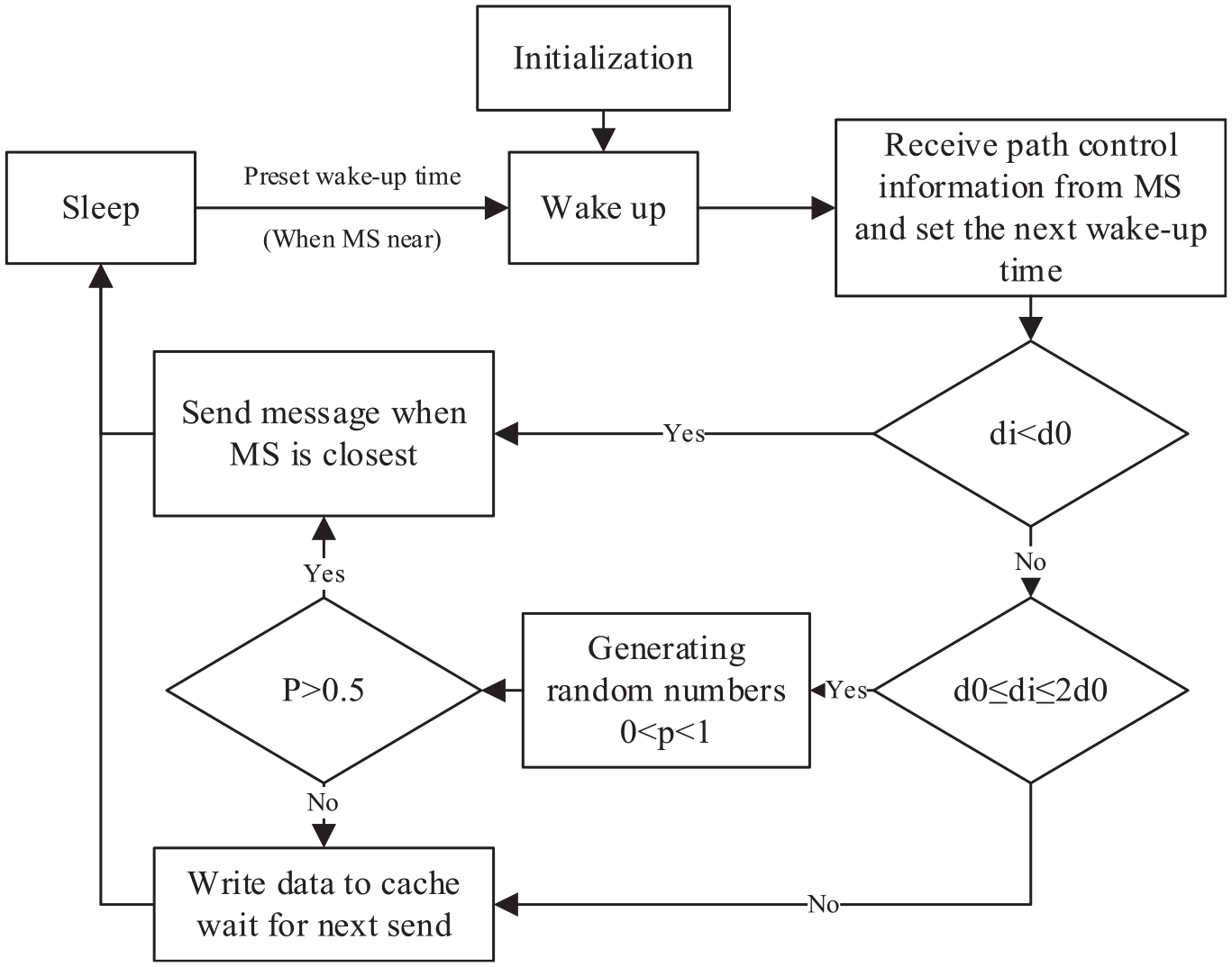
Diagram of the monitoring node state transition.

Simulation and results

According to the information as mentioned above, we simulate the MS-based farmland WSN with an agricultural UAV as the carrier of mobile sink. Table 2 reports the simulation parameters,^32–34 and assumptions of simulation are described in section ‘Basic network hypothesis’. In simulation, VPFBS mobile strategy and distance probability transmission strategy (DPTS) routing protocol are used.

Table 2.

Simulation parameters.

Parameter	Value
Simulation area	$W \times W = 1000 m \times 1000 m$
Initial energy of nodes	$E_{0 i} = 0.5 J$
Number of nodes	$N = 1000$
Data generation rate of node i	$L_{i} = normrnd (1024, 10) bit / h$
Sink node movement rate	$v = 10 m / s$
Distance threshold	$d_{0} = 88.7 m$
Multi-path channel parameter	$ε_{mp} = 0.0013 pJ / (bit \cdot m^{4})$
Frees pace channel parameter	$ε_{fs} = 10 pJ / (bit \cdot m^{2})$
Energy consumption on circuit	$E_{clc} = 50 nJ / bit$

In order to investigate the relationship between the number of RPs and the maximum path length of the MS, we determine the variations in the average length D_mean and maximum length D_max of a single-round path with NR (Figure 9 and Table 3). The length of a single-round path is observed to increase with the number of RPs. The ‘maximum-farthest’ strategy is adopted when selecting the RPs, resulting in a ‘dispersed’ distribution of RPs and a relatively stable increasing trend of the path length.

Figure 9.

Variation of path length with number of RPs.

Table 3.

Variation of path length with number of RPs.

NR	5	10	15	20	25	30	35	40
Average pathlength (m)	1774.6	2608.6	3002.9	3334.1	3562.3	3858.5	4098.9	4302.0
Maximum pathlength (m)	2615.0	3087.1	3303.6	3557.8	3829.8	4029.6	4337.5	4483.2
NR	45	50	55	60	65	70	75	80
Average pathlength (m)	4480.4	4737.4	4973.7	5323.3	5558.3	5920.6	6211.4	6515.3
Maximum pathlength (m)	4713.6	4970.7	5208.8	5560.9	6032.0	6316.9	6631.5	7200.7

NR: number of RPs.

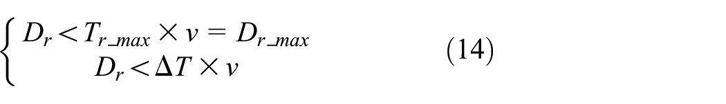
Based on the description in section VPFBS Part C, the single-round endurance of MS D_{r_max} must satisfy the following equation

\begin{matrix} D_{r_\max} = T_{r_\max} \times v > 1.1 \times max (path_length) \\ = path_length_threshold \end{matrix}

(16)

Table 4 details the minimum D_{r_max} required to select NR. In practical applications, the range of suitable RP numbers can be determined in accordance with the situation of the mobile carrier.

Table 4.

Path length thresholds for different values of NR.

NR	5	10	15	20	25	30	35	40
Pathlength threshold (m)	2876.5	3395.8	3634.0	3913.6	4212.8	4432.6	4771.3	4931.5
NR	45	50	55	60	65	70	75	80
Pathlength threshold (m)	5185.0	5467.8	5729.7	6117.0	6635.2	6948.6	7294.7	7920.8

NR: number of RPs.

When the number of RP changes, the distance d between the node and mobile path directly affects the energy consumption and energy balance of the nodes.

Figure 10(a) depicts the relationship between the mean and median of transmission distance d and NR. When NR is less than or equal to 25, the mean and median of d decrease sharply as values of NR increase, indicating the key role of NR in the energy consumption and lifetime of the entire network. As NR continues to increase, d decreases slowly, reducing the impact of NR on the overall performance of the network. This needs to be weighed against the cost of increasing NR and the improvement of energy consumption. In addition, the median of d is significantly smaller than the equivalent mean values, indicating that the RP selection strategy enables the majority of the nodes to be as close to the path as possible. Despite the few nodes that are far away from the path, the RP rotation and probability forwarding mechanisms can avoid the excessive energy consumption of these nodes, thus improving the energy balance performance.

Figure 10.

Variation of statistical values of d with NR: (a) variation of transmission distance with NR and (b) variation of dispersion of transmission distance.

Figure 10(b) demonstrates the variations of the standard deviation and relative standard deviation (RSD) of d with NR. For NR values less than 25, as NR increases, the standard deviation of the node transmission distance decreases and the RSD increases. For NR > 25, the standard deviation of d gradually decreases while the RSD does not change greatly. Thus, as the number of RPs increases, the dispersion of the node transmission distance is reduced. The increasing RSD for N < 25 may be attributed to the visible decrease of the average transmission distance. Furthermore, when NR < 25, increasing the NR values may significantly optimize the energy consumption performance.

Accordingly, the simulation data related to the transmission distance d are shown in Table 5.

Table 5.

Variation of statistical values of d with NR.

NR	5	10	15	20	25	30	35	40
Average of d (m)	179.76	129.03	110.47	89.41	86.49	77.42	69.67	64.97
Median of d (m)	158.82	108.09	89.48	74.08	67.35	61.82	56.47	52.27
RSD of d	0.74	0.78	0.80	0.82	0.84	0.83	0.82	0.83
Standard deviation of d	0.66	0.57	0.50	0.42	0.39	0.35	0.32	0.28
NR	45	50	55	60	65	70	75	80
Average of d (m)	58.84	55.47	52.13	50.44	48.01	45.71	42.73	42.37
Median of d (m)	47.59	44.35	41.86	40.77	38.50	36.42	35.34	34.35
RSD of d	0.84	0.85	0.84	0.84	0.85	0.85	0.83	0.85
Standard deviation of d	0.24	0.21	0.19	0.18	0.15	0.14	0.11	0.11

NR: number of RPs; RSD: relative standard deviation.

We investigate variations in the proportion of nodes with transmission distance d greater than threshold d₀ and 2d₀ in order to determine the proportion of nodes that transmit information in the current round. The proportion of nodes with d > d₀ decreases from 66.38% for 5 RPs to 11.13% for 80 RPs, while for d > 2d₀, the proportion is reduced from 14.49% to 0.52% (Figure 11 and Table 6). As NR increases, the MS path is closer to the nodes, with nodes transmitting data in the current round. Based on the energy consumption model and the data transmission strategy, it can be inferred that as NR increases, the transmission energy consumption decreases, and the probability of a package waiting for the next round is subsequently reduced.

Figure 11.

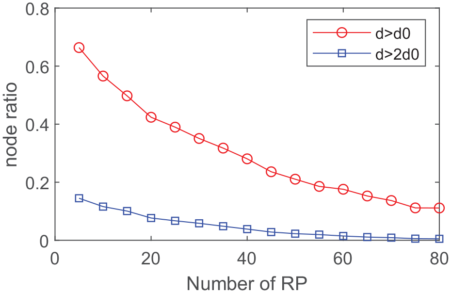
Node proportion trend for d > d₀ and d > 2d₀.

Table 6.

Node proportion trend for d > d₀ and d > 2d₀.

NR	5	10	15	20	25	30	35	40
d > d₀	66.38%	56.57%	49.76%	42.38%	38.97%	35.07%	31.75%	28.06%
d > 2d₀	14.49%	11.60%	10.07%	7.67%	6.72%	5.85%	4.85%	3.86%
NR	45	50	55	60	65	70	75	80
d > d₀	23.61%	21.05%	18.56%	17.58%	15.26%	13.70%	11.16%	11.13%
d > 2d₀	2.84%	2.28%	1.97%	1.48%	1.11%	0.91%	0.56%	0.52%

NR: number of RPs.

In order to observe the information collection in real time, Figure 12 presents the simulation results of the real-time data performance across NR values. As NR increases, the proportion of nodes that can complete the message transmission in the current round increases from 53.53% for 5 RPs to 92.21% for 80 RPs. In addition, the node proportion for two (more than two) rounds decreases from 34.11% to 7.4% (12.36% to 0.38%). Hence, for NR > 15, more than 90% of nodes can control the delay within two rounds. This can essentially meet the real-time requirements of large-scale farmland management.

Figure 12.

Variation of real-time transmission probability with NR.

For large-scale farmland monitoring applications with weak infrastructure, the network lifespan is considered as the most important performance indicator of WSNs. Figure 13 and Table 7 present the network lifespan simulation results. The lifespan is observed to increase with NR, particularly for NR < 40. This has an impact on the increase of the network lifespan.

Figure 13.

Network lifespan changes with NR.

Table 7.

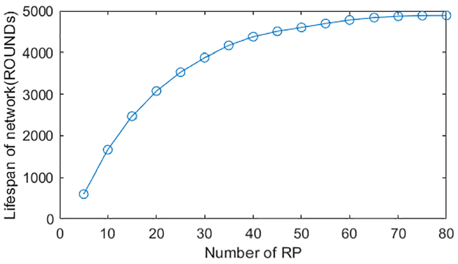
Network lifespan changes with NR.

NR	5	10	15	20	25	30	35	40
Lifespan (ROUNDs)	601	1661	2470	3077	3531	3881	4165	4376
NR	45	50	55	60	65	70	75	80
Lifespan (ROUNDs)	4507	4600	4695	4780	4838	4870	4885	4890

NR: number of RPs.

In order to further observe the changes of surviving nodes during the network operation, we simulated the surviving nodes for NR values of 10, 20, 30 and 40 (Figure 14). The first node and last death nodes appear at (505, 2945) (1090, 4096) and (2615, 4466) (3715, 4785), respectively, while the lifespan R₅₀ is determined as 1661, 3077, 3881 and 4376. Moreover, as the RP number increases, the lifespan of the network is significantly improved and the negative steepness of the curve (reflected by the EBI) increases. In practical applications, this indicates a longer monitoring time and a higher energy balance.

Figure 14.

Number of surviving nodes against rounds.

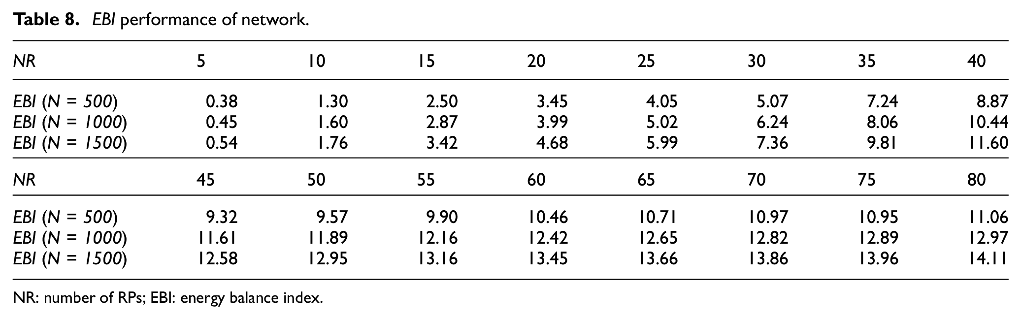
We employ the EBI index to measure the energy consumption balance. The EBI is observed to increase monotonically with NR (Figure 15 and Table 8). In particular, the EBI increases steadily for NR values within the range of 5–30, while for NR values 30–40, this increase becomes steeper and the energy consumption balance of network nodes is partially optimized. The EBI then adopts a gradual increasing trend for NR values greater than 45. For different initial number of nodes, EBI increases with the total number of nodes. Based on these results, an NR value close to 40 can achieve a satisfactory EBI.

Figure 15.

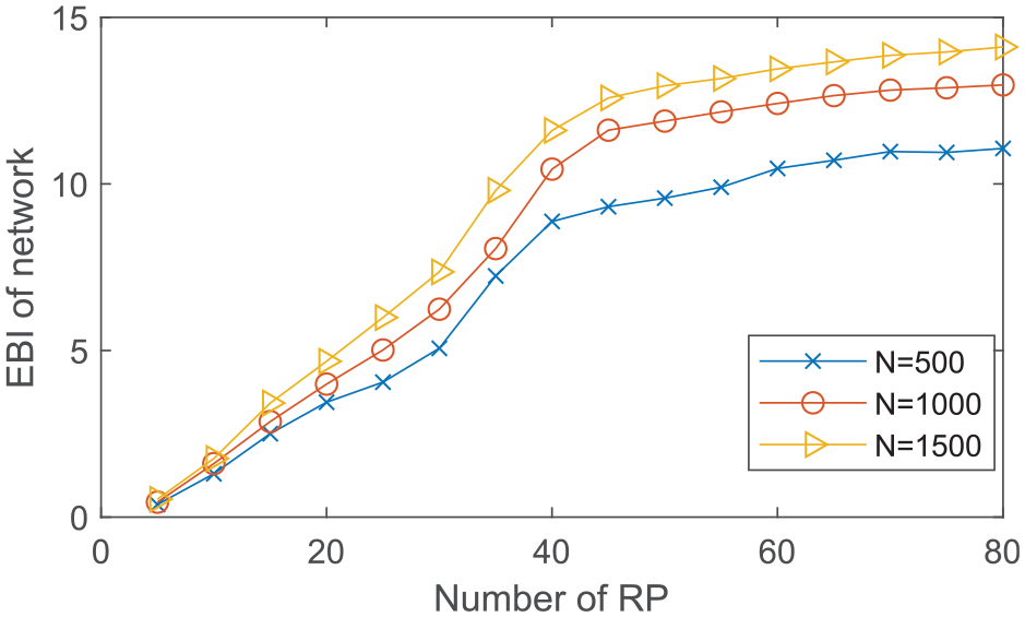
EBI performance of network.

Table 8.

EBI performance of network.

NR	5	10	15	20	25	30	35	40
EBI (N = 500)	0.38	1.30	2.50	3.45	4.05	5.07	7.24	8.87
EBI (N = 1000)	0.45	1.60	2.87	3.99	5.02	6.24	8.06	10.44
EBI (N = 1500)	0.54	1.76	3.42	4.68	5.99	7.36	9.81	11.60
NR	45	50	55	60	65	70	75	80
EBI (N = 500)	9.32	9.57	9.90	10.46	10.71	10.97	10.95	11.06
EBI (N = 1000)	11.61	11.89	12.16	12.42	12.65	12.82	12.89	12.97
EBI (N = 1500)	12.58	12.95	13.16	13.45	13.66	13.86	13.96	14.11

NR: number of RPs; EBI: energy balance index.

In order to describe the energy consumption balance of each round more accurately, the standard deviation of relative residual energy of all surviving nodes after each round is calculated. The slower the growth rate and the lower the maximum value, the better the energy balance of the network will be. When NR equals 10, 20, 30, the energy consumption balance improves significantly with the increase of NR (Figure 16). The network lifetime and node death distribution can also be seen from the change of this performance metric.

Figure 16.

Standard deviation of the relative residual energy of each round.

In summary, as NR increases, the mobile path becomes longer, the transmission distance and energy consumption of the nodes get reduced, and the lifespan of the network may increase. For the MS, path length must meet the threshold in Table 3, the NR, target monitoring time T, time accuracy requisites and the single-round interval $Δ T$ can be weighed according to the simulation results of R₅₀. This allows for the network lifespan and data delay requirements to be met under the limitation of MS motion capability.

In terms of computational complexity, unlike machine learning algorithms, which require a lot of iterations, proposed algorithm has polynomial time complexity O(n) and linear space complexity. Moreover, the complexity of the algorithm can be directly affected by adjusting the distance between sampling points and the influence range of each node, so as to meet the requirements of different accuracy and computing time limits.

Conclusion

In the current study, we investigate the data collection of an MS-integrated large-scale farmland WSN under several constraints. We demonstrate the effective collection of information via the delay-allowed WSN using the following strategies: the construction of a virtual potential field based on the state of nodes; the selection of RPs; traversing each RP with a TPS path as the moving path of the MS; and employing a probability transmission strategy based on transmission distance.

Simulation analysis demonstrates that our scheme can collect real-time data effectively in large-scale farmland and realize the design requirements. In practical applications, the trade-off between several indicators can achieve the required energy consumption and network lifetime. As a precondition for the large-scale application of precision agriculture, the farmland WSN data collection scheme proposed in this study achieves real-time and effective collection of farmland information, adapts to the development requirements of modern agriculture intellectualization and fine industrialization. It can be said that the proposed strategy has a good application prospect. Due to constraints in time, we are unable to perform further optimizations, such as designing RP selection criteria according to real-time requirements, varying the number of RPs across the network operation stages and performing RP rotation at different intervals to reduce overhead costs. These problems will be the focus in future research.

Footnotes

Handling Editor: Dr Peio Lopez Iturri

Declaration of conflicting interests

The author(s) declared no potential conflicts of interest with respect to the research, authorship and/or publication of this article.

Funding

The author(s) disclosed receipt of the following financial support for the research, authorship and/or publication of this article: This work was supported in part by the National Natural Science Foundation of China under Grant 61871041, in part by the Project of Agricultural Equipment Department of Jiangsu University under Grant 4111680005, in part by the Beijing Science and technology project under Grant Z191100004019007 and in part by the Youth Found of Beijing Academy of Agriculture and Forestry Sciences under Grant QNJJ202030.

ORCID iD

Ying Yang

Data availability

The data used to support the findings of this study are available from the corresponding author upon request.

References

Hady

. Duty cycling centralized hierarchical routing protocol with content analysis duty cycling mechanism for wireless sensor networks. Comput Syst Sci Eng 2020; 35: 347–355.

Tabatabaei

. A novel fault tolerance energy-aware clustering method via social spider optimization (SSO) and fuzzy logic and mobile sink in wireless sensor networks (WSNs). Comput Syst Sci Eng 2020; 35: 477–494.

Vijayalakshmi

Anandan

. Global levy flight of cuckoo search with particle swarm optimization for effective cluster head selection in wireless sensor network. Intell Autom Soft Co 2020; 26: 303–311.

Gao

Zhang

, et al. Maximum data generation rate routing protocol based on data flow controlling technology for rechargeable wireless sensor networks. Comput Mater Con 2019; 59: 649–667.

Wang

Gao

Yin

, et al. An enhanced PEGASIS algorithm with mobile sink support for wireless sensor networks. Wirel Commun Mob Com 2018; 2018: 9472075.

Luo

Hubaux

J-P

. Joint mobility and routing for lifetime elongation in wireless sensor networks. In: Proceedings of the IEEE 24th annual joint conference of the IEEE computer and communications societies, Miami, FL, 13–17 March 2005. New York: IEEE.

Somasundara

Kansal

Jea

, et al. Controllably mobile infrastructure for low energy embedded networks. IEEE T Mobile Comput 2006; 5: 958–973.

Shah

Roy

Jain

, et al. Data MULEs: modeling a three-tier architecture for sparse sensor networks. In: Proceedings of the 1st IEEE international workshop on sensor network protocols and applications, Anchorage, AK, 11 May 2003, pp.30–41. New York: IEEE.

Sun

, et al. HUMS: an autonomous moving strategy for mobile sinks in data-gathering sensor networks. EURASIP J Wirel Comm 2007; 2007: 064574.

10.

Sun

. BoSS: a moving strategy for mobile sinks in wireless sensor networks. Int J Sens Netw 2009; 5: 173–184.

11.

Huang

Liu

. A genetic algorithm based strategy for mobile sinks in wireless sensor networks. J Comput Theor Nanos 2011; 4: 3528–3536.

12.

Nguyen

Van Nguyen

. Efficient approach for maximizing lifespan in wireless sensor networks by using mobile sinks. ETRI J 2017; 39: 353–363.

13.

Wang

Zhang

Shen

, et al. An improved stable election based routing protocol with mobile sink for wireless sensor networks. In: Proceedings of the 2013 IEEE international conference on green computing and communications and IEEE internet of things and IEEE cyber, physical and social computing, Beijing, China, 20–23 August 2013. New York: IEEE.

14.

Chhieng

Wong

Fong

, et al. Autonomous path based data acquisition in sensor networks. J Supercomput 2016; 72: 4021–4042.

15.

Reiser

Paraforos

Khan

, et al. Autonomous field navigation, data acquisition and node location in wireless sensor networks. Precis Agric 2017; 18: 279–292.

16.

Cheng

. Data gathering in wireless sensor networks: a combine–TSP–reduce approach. IEEE T Veh Technol 2016; 65: 2309–2324.

17.

Chu

W-C

Ssu

K-F

. Sink discovery in location-free and mobile-sink wireless sensor networks. Comput Netw 2014; 67: 123–140.

18.

Wang

Gao

Zhou

, et al. Optimal coverage multi-path scheduling scheme with multiple mobile sinks for WSNs. Comput Mater Con 2020; 62: 695–711.

19.

Donta

Amgoth

Annavarapu

CSR

. An extended ACO-based mobile sink path determination in wireless sensor networks. J Amb Intel Hum Comp. Epub ahead of print 13 October 2020. DOI: 10.1007/s12652-020-02595-7.

20.

Donta

Rao

BSP

Amgoth

, et al. Data collection and path determination strategies for mobile sink in 3D WSNs. IEEE Sens J 2020; 20: 2224–2233.

21.

Sha

Qiu

, et al. Virtual region based data gathering method with mobile sink for sensor networks. Wirel Netw 2018; 24: 1793–1807.

22.

Liu

Zhang

Shen

, et al. GEERM: an improved grid-based energy-efficient routing method for WSN with single controlled mobile sink, http://icact.org/upload/2016/0264/20160264_finalpaper.pdf

23.

Kostin

Fanaeian

Al-Wattar

. Anycast tree-based routing in mobile wireless sensor networks with multiple sinks. Wirel Netw 2016; 22: 579–598.

24.

Wang

Gao

Liu

, et al. Energy efficient routing algorithm with mobile sink support for wireless sensor networks. Sensors 2019; 19: 1494.

25.

Jiang

, et al. SEBAR: social-energy-based routing for mobile social delay-tolerant networks. IEEE T Veh Technol 2017; 66: 7195–7206.

26.

Jacquet

Mans

Rodolakis

. Information propagation speed in mobile and delay tolerant networks. IEEE T Inform Theory 2010; 56: 5001–5015.

27.

Yun

Xia

. Maximizing the lifetime of wireless sensor networks with mobile sink in delay-tolerant applications. IEEE T Mobile Comput 2010; 9: 1308–1318.

28.

Wang

Cao

Sherratt

, et al. An improved ant colony optimization-based approach with mobile sink for wireless sensor networks. J Supercomput 2018; 74: 6633–6645.

29.

Sharma

Puthal

Jena

, et al. Erratum to: rendezvous based routing protocol for wireless sensor networks with mobile sink. J Supercomput 2017; 73: 1189–1191.

30.

Suh

Berber

. Rendezvous points and routing path-selection strategies for wireless sensor networks with mobile sink. Electron Lett 2016; 52: 167–169.

31.

Yomo

Asada

Miyatake

. On-demand data gathering with a drone-based mobile sink in wireless sensor networks exploiting wake-up receivers. IEICE T Commun 2018; E101B: 2094–2103.

32.

Jan

Hameed

Ali

, et al. A balanced energy consuming and hole alleviating algorithm for wireless sensor networks. In: Proceedings of the 2017 31st international conference on advanced information networking and applications workshops (WAINA), Taipei, Taiwan, 27–29 March 2017. New York: IEEE.

33.

Naranjo

PGV

Shojafar

Mostafaei

, et al. P-SEP: a prolong stable election routing algorithm for energy-limited heterogeneous fog-supported wireless sensor networks. J Supercomput 2017; 73: 733–755.

34.

Tunca

Isik

Donmez

, et al. Ring routing: an energy-efficient routing protocol for wireless sensor networks with a mobile sink. IEEE T Mobile Comput 2015; 14: 1947–1960.

A mobile sink–integrated framework for the collection of farmland wireless sensor network information based on a virtual potential field

Abstract

Keywords

Introduction

Related work

Scenario assumptions and parameter descriptions

Basic network hypothesis

Data transmission characteristics and energy consumption model

Network lifetime and energy balance index

Behaviour strategy of nodes in large-scale farmland WSNs

VPFBS: virtual potential field-based strategy for mobile sink path planning

Mobile sink path planning process

Construction of virtual potential field based on multi-factor node states

Attractive potential field from nodes

Repulsion of potential field from edge

Selection and rotation of RPs

Constraints on the number of RPs

Selection of RP location

RP rotation

DPTS: distance probability transmission strategy for monitoring nodes

Simulation and results

Conclusion

Footnotes

Declaration of conflicting interests

Funding

ORCID iD

Data availability

References