Sage Journals: Discover world-class research

Abstract

To explore the development mechanism of cracks in the process of rock failure, triaxial compression tests with simultaneous acoustic emission monitoring were performed on granite specimens using the MTS rock mechanics test system. The frequency-domain information of the acoustic emission signal was obtained by the fast Fourier transform. The Gutenberg–Richter law was used to calculate the acoustic emission signals and obtain the b-value dynamic curve in the loading process. Combined with the stiffness curve of granite specimens and acoustic emission signal in the time domain and frequency domain, the crack development characteristics in different stages were analyzed. The results showed that the acoustic emission signals of granite samples under triaxial compression can be divided into four stages: quiet period 1, active stage 1, quiet period 2, and active stage 2. b-value attained its maximum value in the active phase 2 when it is close to the sample loss, and then drops rapidly, which means the propagation of cracks and the formation of large cracks. The acoustic emission signal’s dominant frequency was not more than 500 kHz, mostly concentrated in the medium-frequency band (100–200 kHz), which accounted for more than 80%. The proportion of signals in each frequency band can reflect the distribution of the three kinds of cracks, while the change in low-frequency signals can reflect the breakthrough of microcracks and the formation time of macrocracks in granite samples. By fully analyzing the characteristics of acoustic emission signals in the time domain and frequency domain, the time and conditions of producing large cracks can be determined accurately and efficiently.

Keywords

Dominant frequency granite triaxial compression Fourier transform crack identification

Introduction

The occurrence of failure is a process from quantitative change to qualitative change, and the fracture of the rock mass is also a process from microcrack to macrocrack. In the process of rock fracture, the energy stored in the rock was released in the form of an elastic wave during the formation of structural defects such as fractures, twins, and dislocations. Moreover, the mechanical properties of the rock are greatly affected by the initiation and development of large cracks. Therefore, it is imperative to adopt a monitoring technology that can accurately and efficiently reflect the timing of the initiation and occurrence of large-scale cracks in rocks in real-time.

With the growing complexity of geological conditions in slope, underground tunnel, and coal mine, accidents such as land slide and collapse occurred frequently. The acoustic emission (AE) signal will be produced in the process of deformation and the failure of the surrounding rock and mine roadway.^1–3 AE technology can detect the cracks produced by deformation without delay.^4,5 Nowadays, as an effective monitoring method, AE technology has been widely used in the geotechnical field.^3,6–8

To understand the AE characteristics of rock materials during deformation, researchers conducted many investigations on AE characteristics with different rock or rock-like materials. For example, literature^9–12 described the failure process of concrete and rock-like materials by analyzing time-domain signals such as the amplitude, energy, ringing number, and event number of AE signals. Schiavi et al.¹³ calculated theb-value dynamic curve of AE amplitude information using Gutenberg–Richter law and analyzed the damage process of compression concrete specimens. However, the relationship between the fracture type and these time-domain parameters has not been determined yet. This will bring some difficulties to the prediction and location of rock fracture types and even fractures. At the same time, the AE frequency domain can reflect the propagation form of rock fracture and indirectly reflect the propagation process of the internal stress field.^6,14–16 Therefore, the AE spectrum characteristics have gradually become an essential means of the interpretation of the rock failure mechanism.¹⁷

Due to the rapid development of computer processors and sensors, the AE waveform has been studied extensively. When the rock is in the triaxial compression state, the primary fracture is a shear crack, while tensile crack exists at the same time.^18,19 Zang et al.²⁰ investigated the microscopic mechanism of rock failure and proposed the first motion polarity method and moment tensor method. The results showed that the low dominant frequency waveform (L-shaped waveform) is generated by microtensile crack, and the high dominant frequency waveform (H-shape waveform) is caused by microshear crack. Rathnaweera et al.²¹ and Cai et al.²² found that the frequency of stress release wave could reflect not only the type of crack but also the size of crack. Subsequently, Schiavi et al.¹³ studied the frequency information of elastic waves in the compression process of concrete specimens from both microscopic and macroscopic aspects and found that the low-frequency signals appearing before the failure could represent the sudden transition from microcracks to locally distributed macrocracks, symbolizing the catastrophic failure of brittle materials. Through research, Wang et al.²³ also found that the frequency is inversely proportional to the crack size. That is, the high-frequency AE signal corresponds to the initiation of microcracks, while the low frequency is related to the formation of large cracks. Therefore, AE signals released by rocks during loading, especially frequency-domain information, can effectively describe the crack morphology of rocks.

As mentioned above, the time series characteristics of AE have been widely studied, and the time and frequency analysis of AE monitoring is expected to be one of an essential means to study the formation mechanism of internal cracks in the rock mass. Nonetheless, to date, little attention has been paid to the combination of the time domain and frequency domain with the development stage of rock fractures. The development of fractures runs through the whole process of rock loading. Through the basic parameters (ringing count, event number, absolute energy, cumulative count, etc.) of AE, the evolution characteristics of rock fracture occurrence can be obtained. In addition, by analyzing the frequency-domain characteristics of AE (dominant frequency, the amplitude of dominant frequency, etc.), the specific shape of fracture in the process of rock fracture incubation can be obtained. Thus, it is reasonable and necessary to carry out the time–frequency and b-value analysis of AE combined with several rock loading stages, especially for different frequencies.

In this article, triaxial compression tests with synchronous AE measurements were carried out on granite samples. The time-domain and frequency-domain information of AE signals were first analyzed using fast Fourier transform (FFT) and Gutenberg–Richter law. The relationship between fracture type and occurrence time and AE signal under the triaxial state of granite was then fully discussed. This study can be used to provide a more efficient and economical method for determining the time and conditions of producing large cracks.

Test system and analysis method

Test device

All the tests involved were carried out with the MTS815.04 rock mechanics experimental system (Figure 1). The bearing capacity and confining pressure of the system can reach 4600 kN and 140 MPa, respectively. Axial force (given by the load cell, with a range of 1000 kN), axial deformation, and lateral displacement were monitored in real-time during the test. The axial deformation was monitored by a linear variation difference instrument (LVDT) (Figure 1), and the lateral deformation was measured by the circumferential extensometer (632.12f-20) of the MTS test system. As shown in Figure 1, the axial and circumferential LVDT were located in the middle of the granite sample to eliminate the end friction effect.²⁴

Figure 1.

MTS loading device.

The PAC company’s PCI-II AE system was used to monitor the waveform and positioning information in the whole loading process. The system has ten independent channels with a bandwidth of 1 kHz–3 MHz and a sampling frequency of 1 MHz. Six micro30 sensors receive the relevant parameters during the test, as shown in Figure 2(a). The sensor has good frequency response characteristics and sensitivity to the AE signal. Six AE sensors were arranged in two layers; each layer is 20 mm away from the end. Each sensor in same layer is 120° adjacent to each other, and the arrangement point is shown in Figure 2(c).

Figure 2.

Layout of acoustic emission device and acoustic emission probe: (a) acoustic emission sensor, (b) acoustic emission amplifier, and (c) acoustic emission sensor layout.

Test material and specimen installation

To investigate the crack development characteristics of granite samples under triaxial compression, simultaneous AE tests were carried out. The granite in Miluo City, Hunan Province, China, was selected for this test. According to ISRM’s recommendation, the required rock samples were made into 50 mm× 100 mm cylinders for the triaxial compression test. The density of granite is approximately 2.87 g/cm³. To keep the sample in its original state and prevent oil from entering the triaxial cell during loading, which will change the pore pressure state and loading environment of the sample, heat-shrinkable sleeve sealing treatment was carried out, as shown in Figure 1 (right).

After the sample was made, the MTS axial displacement meter, circumferential displacement meter, and PAC AE sensors were installed. To ensure the accuracy of the test data, the testing machine and the AE main box were grounded at the same time to reduce the environmental noise interference. Finally, as shown in Figure 2, the preamplifier had a gain of 40 dB and a threshold of 45 dB. The relevant parameters of each channel were consistent. During the test, Vaseline was applied between the sensor and the sample to ensure that the sensor and the sample were fully coupled. In addition, before the test, the probe’s sensitivity was checked, and the probe was positioned. The AE signal emitted by rock fracture was simulated using an automatic pencil of 0.5 mm, a 2.5-mm nib, and a 30°-angle fracture on the surface of the sample. The break lead point’s relative position and the preset probe were observed in AE-win software, and the average wave velocity was adjusted to make it close to the probe.

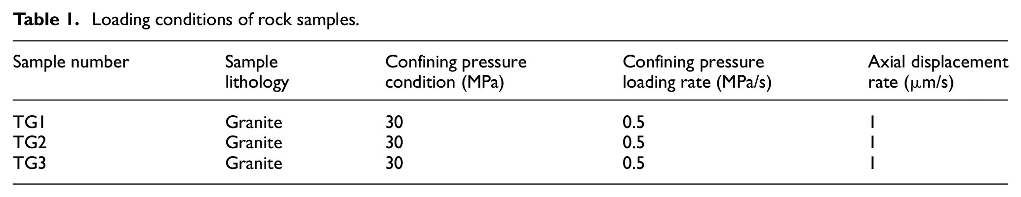
The loading mode was 0.001 mm/s, as recommended by ISRM, and the axial displacement was applied. The test scheme is shown in Table 1. Before loading, the sample was prepressed and fixed to prevent the sample from moving during oil injection. After the oil injection, the air in the triaxial chamber was removed to avoid influencing the test. The confining pressure was raised to the target confining pressure of 30 MPa at the rate of 0.5 MPa/s.

Table 1.

Loading conditions of rock samples.

Sample number	Sample lithology	Confining pressure condition (MPa)	Confining pressure loading rate (MPa/s)	Axial displacement rate (μm/s)
TG1	Granite	30	0.5	1
TG2	Granite	30	0.5	1
TG3	Granite	30	0.5	1

AE data acquisition and analysis method

As shown in Figure 3, a set of data was collected by the system’s acquisition board for each fracture initiation in the loading process. The PCI-II system recorded the collected AE waveform data as a separate data file. Using MATLAB programming, the AE waveform data were obtained by FFT and converted into the spectrum. The AE waveforms’ dominant frequencies were calculated by the batch processing method, and Excel tables were automatically exported.

Figure 3.

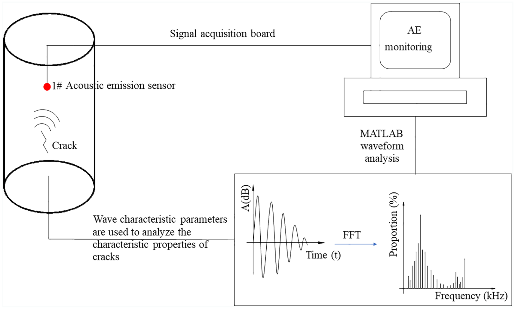
AE data processing technology flowchart.

FFT was used to transform the waveform signal generated by fracture into the frequency-domain signal. The fractured form was analyzed by combining the dominant frequency information. At the same time, the Gutenberg–Richter law was used to calculate the AE amplitude information to obtain the granite crack propagation scale function—b-value under triaxial compression. Finally, dynamic b-value changes in the dominant frequency of AE fracture and the whole loading process were analyzed to identify crack initiation, propagation timing, and fracture types under triaxial compression.

Test results

Mechanical properties

The axial stress–strain curves and related parameters of the target granite samples are illustrated and listed in Figure 4 and Table 2. Figure 4 shows that the dispersion of the target samples was not very large. The statistical data of the mechanical parameters in Table 2 show that the mean square deviation of the test samples was within a reasonable range and was statistically significant. Therefore, it is appropriate to select a group of representative data for further analysis.

Figure 4.

Axial stress–strain curves of granite tested under triaxial compression.

Table 2.

Statistics of mechanical properties of test samples.

Sample	Maximum principal stress (MPa)	Peak strain (%)	Elastic modulus (GPa)
TG1	402.19	0.79	55.28
TG2	378.45	0.88	59.15
TG3	389.44	0.82	56.42
Average	389.96	0.83	56.95
Variance	138.85	2.1e−5	3.95
Standard deviation	11.783	0.0458	1.989
Proportion (%)	3.02	5.52	3.49

Figure 5 shows the stress–strain relationship, the relationship between stress and volume strain, the relationship between axial strain and volume strain, and the stiffness curve of granite samples in the triaxial state for the whole process. From the stress–strain relationship curve, it is evident that the curve changed from the initial microconcave shape to the straight-line state then turned to the convex shape and finally dropped. Moreover, by comparing the relationship between axial strain and volumetric strain and the stiffness curve for the whole process, the whole process of triaxial compression can be divided into four stages: the compaction stage, elastic stage, yield stage, and failure stage. As shown in Figure 5, combined with the stiffness curve for the loading process, the stress state corresponding to each stage node can be qualitatively defined as crack closure stress, σ_cc, damage stress, σ_cd, and peak stress, σ_c.^25–27 The compaction effect of internal pores was observed when the sample was in the compaction state. At this time, the stiffness of the granite sample decreased a little and then increased rapidly. Interestingly, the damage stress threshold, σ_cd, corresponded to the inflection point of the volume strain. That is, when the stress state exceeded the damage stress threshold, the specimen changed from the initial compression state to the volume expansion. This means that the specimen was damaged and a large number of new cracks were initiated. At this time, the granite sample’s stiffness decreased immediately until macroscopic fracture or a loss of stability occurred.

Figure 5.

Stress–strain diagram showing the four stages of crack development.

Analysis of crack morphology

As shown in Figure 6, the elements in the rock mass were subjected to the combined action of normal stress and shear stress to produce the principal stress. According to the stress transformation equations in material mechanics,²⁸ the relationship between normal stress, shear stress, and principal stress was as follows

σ_{α} = \frac{σ_{x} + σ_{y}}{2} + \frac{σ_{x} - σ_{y}}{2} \cos 2 α - τ_{x} \sin 2 α

(1)

τ_{α} = \frac{σ_{x} - σ_{y}}{2} \sin 2 α + τ_{x} \cos 2 α

(2)

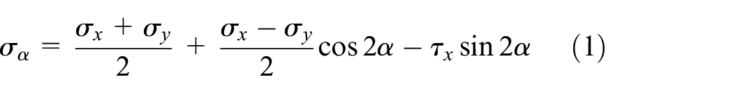
When the element could be stressed in the tangential direction, it was brought into the stress transformation law (1). In order to maximize the normal stress, namely, sin2α = 1, the angle α = 45° was calculated. That is, the angle between the direction of crack development and the axial direction was approximately 45°, shown as the dotted line in Figure 6, and the crack type was a shear crack. Similarly, when the element was subjected only to normal stress, the stress transformation equations was used to calculate α = 0° or 90°. That is, the crack development was approximately horizontal or vertical, as shown in Figure 6 (right), and the crack type was a tensile crack.

Figure 6.

Element stress analysis and crack morphology diagram.

However, in the actual rock mass, the unit body was subjected to the joint action of normal stress and shear stress at the same time, resulting in the primary normal stress and main tangential stress. When the principal stress was greater than the strength of the element, the crack developed along the principal stress’s vertical direction. Crack extension was affected by many factors, such as rock structure, heterogeneity, stress pattern, and so on. Nevertheless, for rocks with little structural change, the impact of load on the crack plays a key role, and the analysis of crack morphology can reflect the load-bearing form to a certain extent, that is, the approximate crack type can be judged. For example, when the principal stress was greater than the principal tangential stress, σ_α > τ_α was brought into the stress transformation equations, the angle α was less than 45°. The crack type with low angle can be roughly regarded as the tensile–shear crack. The crack strike was also perpendicular to the primary normal stress direction, but mainly tensile crack. When the principal tangential stress was greater than the principal normal stress, σ_α < τ_α was brought into the stress transformation equations, and the angle α > 45° was obtained. Similarly, considering the non-uniformity of rock materials, the crack form with a large angle can be roughly regarded as the tensile–shear crack. The crack strike was also perpendicular to the main normal stress, but mainly shear crack.

Considering that the stress of rock mass under triaxial compression is in accordance with Mohr–Coulomb criterion. In the actual rock mass fracture form, the internal friction angle of the rock sample should be considered, that is, in the actual state, the failure form of the main crack should be shear crack, and the angle should be 45°+φ/2. However, due to the heterogeneity of the rock, structural differences, and other factors, the internal force of the unit body changes, that is, the appellate stress state is likely to occur. Therefore, in the process of rock fracture, all three types of cracks exist.

As shown in Figure 7, the red line can roughly represent the main shear crack of granite under triaxial compression. It should be noted that besides the main shear crack, it also contains tiny cracks at various angles. For example, in Figure 7 (TG-2), there were microcracks with different angles around the main shear crack. And those cracks whose angle is close to horizontal or vertical can be roughly judged as tensile crack. The rest of the cracks can be roughly regarded as tensile–shear cracks. Furthermore, the other two rock samples also have three types of crack morphology.

Figure 7.

Macrocracks diagrams of samples.

Analysis of time and frequency characteristics of AE

Time-domain analysis of AE

Figure 8(a)-(d) shows the time-domain signal of granite’s AE and the characteristics of stiffness and stress during loading process. Several obvious and exciting phenomena can be found through comparative analysis. According to the changing trend in mechanical properties and AE characteristic parameters, the crack development of granite under triaxial compression can be divided into four stages: quiet period 1 (crack closure), active stage 1 (crack initiation), quiet period 2 (crack stable propagation), and active stage 2 (crack unstable propagation).

Figure 8.

Characteristic diagram of AE time-domain signal and stiffness and stress during loading. (a) AE amplitude, (b) AE energy, (c) AE impact rate, and (d) local AE impact rate.

Due to the existence of initial pores in the specimen and the slight friction between the end of the specimen and the loading indenter, the specimen’s stiffness changed significantly during the stage I. The stiffness curves decreased first and then increased to the initial stiffness. In this stage, a low-amplitude, low-energy impact occurred occasionally, and the energy duration was very short. At this time, the activity of AE was weak and in a quiet period.

During the stage II, the rock mass’s original cracks were further compacted, and no damage was caused to the rock mass. The rock sample became progressively denser, and the mechanical properties became progressively stronger. The stiffness of the sample continued to increase until it reached the maximum value (50.8 GPa). In this process, the AE parameters, such as amplitude, number of hits, energy, and other characteristic parameters, began to change. In particular, the energy and impact rate increased significantly compared with the previous stage. This marks the first active period of AE.

At the end of the stage II, the sample’s stiffness reached its peak and then began to fall. It indicates that the samples’ AE characteristics have entered another stage, a relatively quiet period. At this stage, the specimen’s stress state exceeded the volume strain reverse bending point (damage stress threshold, σ_cd). However, the damage degree was limited. As a result, the impact rate, energy, and amplitude of the AE were limited, the signals with low energy and high amplitude appeared occasionally, and the duration was very short.

With the further development of the test, the cleavage planes of minerals, such as biotite and feldspar, promote the weak plane’s further development. When the sample’s stiffness was lower than the initial stiffness, that is, when the strain reached 0.65%, another active period was entered. At this stage, the energy, amplitude, and impact rate of the AE increased obviously. The impact rate increased exponentially with the amplitude of 100 dB. Energy also increased sharply, breaking through 6e10 (aJ). This was because the soft surface produced massive dislocation displacement under the action of high pressure, and significant energy was released. When the load exceeded the peak stress level, the sample was unstable and failed, with cracks produced due to the fracture moving out. The energy, impact rate, and amplitude of AE decreased.

From the perspective of the AE time domain, low-amplitude and low-energy AE signal indicate the generation of microcracks, which had little contribution to the change in the overall mechanical properties of the rock samples. In contrast, it was a high-amplitude and high-energy signal, which corresponds to large fractures and even macrocracks.^29,30 Therefore, the generation of such signals had a significant impact on the rock samples’ overall mechanical properties. In conclusion, AE amplitude and energy can reflect the fracture degree of the crack, while the AE rate can roughly reflect the occurrence time of large cracks. In this experiment, large cracks were most likely to occur in the last active period.

b-value calculation and analysis

As a function to describe the crack propagation scale, AE b-value can be used to track the evolution law of rock fractures. Under triaxial compression, the damage degree inside the rock at different stress stages is different, and the AE characteristics are also quite different. The time-varying b-value can well reflect the changing state of the crack inside the rock at different loading stages, as well as the scale extension of the microcracks inside the rock.^31–33 The G–R relation between magnitude and frequency of seismic activity proposed by Gutenberg and Richter as follows¹³

\lg N = a - bm

where m is the magnitude, N is the magnitude within ΔM—the number of specimens, and a and b are the constants. For the estimation of b-value, the most common method is the maximum likelihood method

b = \frac{\log_{10}^{e}}{\bar{M} - (M_{C} - \frac{Δ M}{2})}

where $\bar{M}$ is the average magnitude, M_c is the final magnitude, ΔM is the magnitude distribution width, and $M_{C} - (Δ M / 2)$ is considered as the initial magnitude level.

As b-value is a statistical value, it is related to the integrity of statistical data, the number of samples, calculation step, and other factors. In this article, AE data of representative specimens in the triaxial compression test at a loading rate of 0.001 mm/s were used. Meanwhile, the scanning algorithm was used to calculate the b-value in the stress deformation of specimens. With a sampling window of 250 and a step length of 50, the b-value sequence of granite samples changing with time was calculated to analyze b-value’s variation characteristics.

The b-value sequence was superimposed with the granite stress–strain curve to analyze the influence of stress state change on the b-value. According to the above analysis results, AE b-values at each stress stage were calculated to examine the internal damage of rocks at different stages and the variation characteristics of AE b-values. As shown in Figure 8, the AEb-values of rocks exhibited various degrees of fluctuation in the four stages. The change process of itsb-value is as follows: (1) When the sample is in the initial compaction stage, namely, the quiet period 1, the b-value presented a downward trend. It means that the primary voids existing in the rock sample are compressed at this stage. (2) When the rock sample is in the elastic stage, the elasticity can be stored in its interior largely, without apparent rupture. Therefore, this stage’s b-value remains constant, which includes the active stage 1 and the calm stage 2. (3) As the load is applied, after the elastic stage, it entered into active stage 2. The b-value began to increase, the crack started to breed, and the microcrack started to sprout, leading to a decrease in the b-value. With the aggregation and penetration of small-scale microcracks and the formation of large-scale cracks, sudden instability occurred. At this time, the value of b showed a trend of sudden decline, shown as the dotted line in Figure 9. Therefore, the fluctuation of b-value can more accurately describe the granite fracture process.

Figure 9.

Stress–strain and b-value curves of granite.

Spectrum analysis of AE signal

Because the AE signal contains a large amount of information, it is not enough to interpret it only from the time domain and b-value. Therefore, based on the monitoring data, the AE parameters and waveform were extracted, and the AE frequency domain was analyzed. Since the AE signal is a nonstationary signal, it can be considered to be composed of numerous sine or cosine signals, expressed as follows

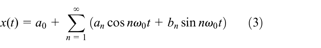
x (t) = a_{0} + \sum_{n = 1}^{\infty} (a_{n} \cos n ω_{0} t + b_{n} \sin n ω_{0} t)

(3)

where n = 1, 2, 3…, $ω_{0} = 2 π / T$ , while $a_{0}$ , $a_{n}$ , and $b_{n}$ are the Fourier coefficients, and the following equations express their values

a_{0} = \frac{1}{T} \int_{- T / 2}^{T / 2} x (t) d t

(4)

a_{n} = \frac{2}{T} \int_{- T / 2}^{T / 2} x (t) \cos n ω_{0} t d t

(5)

b_{n} = \frac{2}{T} \int_{- T / 2}^{T / 2} x (t) \sin n ω_{0} t d t

(6)

Through the sum difference product formula of the sine function and cosine function, the AE signal expression can be simplified into Fourier series with engineering significance, as shown in equation (7)

x (t) = a_{0} + \sum A_{n} \cos (n ω_{0} t + φ_{n})

(7)

where $A_{n} = \sqrt{a_{n}^{2} + b_{n}^{2}}$ is the amplitude of the harmonic component when n = 1, A₁ is the value component of the fundamental wave, $φ_{n} = - \arctan (b_{n} / a_{n})$ is the amplitude of the harmonic component, and a₀ is the DC component.

The frequency spectrum of the periodic signal of the $A_{n} - ω$ diagram (amplitude–frequency diagram) can be obtained by a Fourier expansion. The spectrum of the periodic signal is composed of infinite spectral lines. Each line represents a harmonic component, and its height represents the magnitude of the corresponding harmonic component bat value. Figure 10 is the schematic amplitude spectrum of a signal.

Figure 10.

Amplitude diagram of Fourier transform signal.

The FFT is a classic spectrum analysis method to analyze nonstationary signals. Therefore, FFT technology was used to transform the AE signal waveform into a frequency spectrum, and its dominant frequency and amplitude were statistically analyzed. The frequency corresponding to the highest point of amplitude in the two-dimensional (2D) spectrum was defined as the dominant frequency waveform signal. The highest point of the amplitude was defined as the dominant frequency amplitude. For example, the typical AE waveform (lead breaking signal) and its spectrum are shown in Figure 11. The dominant frequency was 40 kHz, and the amplitude of the dominant frequency was approximately 0.12 dB. Because each rock sample had many AE data sets, batch processing was the key to AE signal processing. In this article, a batch processing program was programmed in MATLAB, which can process many AE waveform files quickly and effectively.

Figure 11.

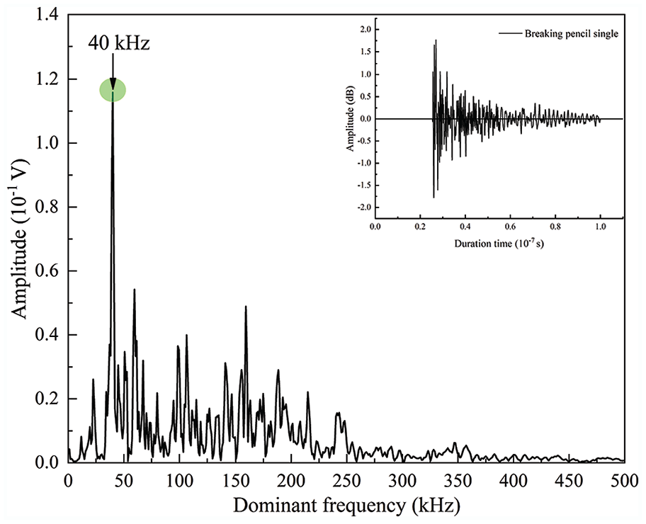
Time–frequency conversion diagram of the lead breaking signal.

In this study, MATLAB software was used to write a batch processing program to identify and read the time domain of all signals automatically. The FFT program was used to convert them into a frequency-domain diagram. Each AE waveform’s dominant frequency was obtained by analyzing the frequency spectrum of the AE waveform of the granite specimen during triaxial compression. The frequency range of the AE waveform after the FFT transformation was 0–500 kHz. The reference band can divide the whole frequency range into three frequency segments: 0–100, 100–200, and 200–500 kHz corresponding to low frequency, intermediate frequency, and high frequency, respectively.³⁴ The dominant frequency and amplitude of dominant frequency were extracted in each batch. Then, the polarity method was used to calculate the number and proportion of different frequencies and amplitudes. Figure 12 shows the histogram of the proportion of triaxial AE signals of granite with six other statistical methods. The comparative analysis of each channel parameter’s proportion shows that the data distribution of channel 1 was relatively complete. Therefore, the parameters collected by channel one was selected as the target object for further research and analysis.

Figure 12.

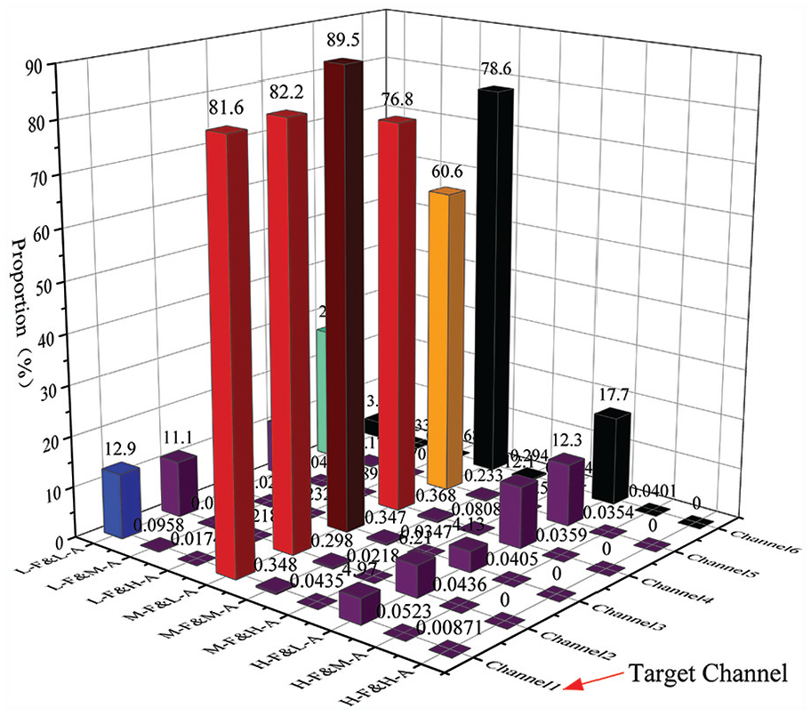
Ratios of main frequency parameters of each channel.

The signal obtained by the target channel was filtered and analyzed by FFT. It was found that the waveforms carry information on the rock mass stress state, structure, physical mechanics, and so on. Figure 13(a)–(d) shows the different stress stages under the triaxial compression of granite. As shown in Figure 13(a), when the AE waveform was in the compaction stage, the amplitudes of the AE signals were low and similar in value. However, the dominant frequencies were 184 and 230 kHz. As shown in Figure 13(b), a phenomenon similar to the compaction stage can be observed when in the elastic stage. That is, the amplitude of each frequency was identical. However, this occurred only after 300 kHz, and the two dominant frequencies were 388.3 and 430 kHz. As shown in Figure 13(c), both the amplitude and the trend were significantly different from the previous two stages when approaching the peak value. The amplitude of the dominant frequency was greater than that of the first two stages, and the dominant frequency changed from multiple frequencies to a single dominant frequency of 40.5 kHz. This was consistent with the dominant frequency and amplitude of the broken lead signal before the test. As shown in Figure 13(d), the spectrum of AE signals at each stage was compared. There were obvious differences: the dominant frequency of AE signals changed from multiple peaks of intermediate frequency to multiple peaks of high frequency and from low compaction stage to elastic stage. With the increase in stress, the dominant frequency shifted from multiple high-frequency peaks to a single low-frequency peak. In particular, AE was mainly manifested as medium- and low-frequency signals with a single dominant frequency when approaching the failure. The dominant frequency was related to the signal attenuation. That is, the higher the main signal frequency was, the more pronounced the signal attenuation was.^13,14,35 However, the signal attenuation of a large-scale fracture was slow, the signal duration of microfractures was short, and the signal decline was substantial. The low-frequency AE signals generated near the failure stage were consistent with the dominant frequency and amplitude of the lead break signal before the test, as shown in Figure 14. Therefore, large-scale cracks usually showed low dominant frequencies, while microcracks showed high dominant frequencies. Consequently, it is believed that this type of signal was likely to be generated by the fracture signal similar to the broken lead, that is, the frequency-domain characteristics of the signal generated by the large crack. Therefore, the occurrence time of a large crack was close to the peak state.

Figure 13.

AE spectrum of granite in different stress stages under triaxial compression: (a) time-domain conversion of the compaction stage, (b) elastic phase time-domain conversion, (c) yield stage time-domain conversion, and (d) signal set near three stress eigenvalues.

Figure 14.

Comparison of lead breaking signal and yield signal: (a) lead breaking signal and (b) yield signal.

The loading process of granite accompanied the initiation, development, and extension of cracks. Based on the AE frequency information, the crack development type can be determined by the development timing, especially the extension time. In this article, the AE frequency was divided into three levels: low frequency (0–100 kHz), intermediate frequency (100–200 kHz), and high frequency (200–500 kHz). Different dominant frequencies reflect the information under other stress states, that is, other fracture forms. Li et al.³⁶ found that, when the dominant frequency of the AE signal is low, tensile cracks will occur; when the dominant frequency is high, shear cracks will appear. The coupling between high frequency and low frequency is the coupling form of tensile fracture and shear crack.

All AE frequencies in the compression process were classified and counted, and the dominant frequency distribution diagram and dominant frequency ratio diagram were drawn, as shown in Figures 15 and 16. The frequency-domain distribution diagram of AE shown in Figure 15 demonstrates that, in the compaction stage, there were fewer high-frequency, medium-frequency, and low-frequency signals. With the further increase in stress until the yield stage, the frequency signals grew. The frequency distribution was most concentrated near the peak value. Then, due to the sample’s instability and failure, the AE probe fell off, reducing the AE signal. However, from the signal collected, the signal was still far beyond the other two frequency bands. Therefore, in the whole loading process, the tension shear coupling cracks were dominant and accompanied by pure tension or pure shear cracks.²⁰

Figure 15.

Dominant frequency distribution of acoustic emission in the whole loading medium.

Figure 16.

Different frequency ratios in the whole loading medium.

Further analysis of the frequency-domain trend chart of AE in Figure 16 shows that the increasing frequency proportion trend was not the same. The dominant frequency signal showed a growing trend. In the initial loading stage, the number of AE events and signals generated by the original fracture’s closure under high confining pressure in the initial compaction stage was less. Therefore, the proportion of the dominant frequency signal was relatively small, which means that the cracks were less developed. The frequency band proportion of this stage shows that the tensile–shear crack was more developed than the tensile crack and shear crack. After entering the elastic stage, the proportion of medium-frequency bands increased rapidly, and the tensile shear-type microcracks sprouted quickly. The formation of microcracks marks the active stage of AE. When the strain rate was 0.5%, the proportion of medium-frequency bands showed a peak, decreased rapidly and increased with the low-frequency band. This means that the rapid development and extension of tensile shear mode microcracks led to tensile shear macrocracks.

With the load applied, when the strain was further increased to 0.77%, the frequency signal accounted for 22%. This means that the microcracks were fully developed and dominated by tensile–shear cracks. In the yield stage, the low-frequency signal also showed a sharp increase, especially in the range of 0.65%–0.85% strain rate, and the proportion of the low-frequency band was up to 5% and then decreased rapidly. This means that the shear cracks corresponding to the low-frequency band germinated, developed rapidly, and passed through in this period. A macroshear crack was formed through the specimen, as shown in Figure 7.

As mentioned above, the variation in each frequency band’s ratio curve can reflect the timing of the breakthrough of microcracks and the formation of large cracks in granite samples. Simultaneously, the failure of microcracks was also an essential reason for the final macrofracture. This also indicates the failure and macrofracture of the specimen, and the macrocrack formation time was close to that shown in the cyan section in Figure 16.

Analysis of main frequency amplitude

The dominant frequency amplitude of the AE was extracted. The amplitude of each dominant frequency under triaxial compression was further analyzed to obtain the amplitude diagram of the dominant frequency of the AE, as shown in Figure 17, demonstrating that the proportion of each dominant frequency amplitude was different. The low-amplitude signal (0.02 V > A) was significantly higher than the medium- and low-amplitude signal. In addition, the changing trend in each dominant frequency amplitude was consistent. In particular, the trend in the low-amplitude signals was more pronounced. This shows that the low-amplitude signal played a dominant role in the AE process of granite. In the whole loading process, for low-frequency signals, the unit time statistics of high-amplitude signals reached 450 hitting’s, which were far more significant than those of medium- and low-amplitude signals. This was because the amplitude of the dominant frequency was closely related to the strength of the AE signal. The stronger the AE signal was, the higher the amplitude was, the weaker the intensity was, and the lower the amplitude was. However, the strength of AE signals showed the generation and development of macro- and microcracks. This further indicates that the high amplitude corresponded to the macroscopic fracture mode.

Figure 17.

Relationship between AE main frequency–amplitude and stress–strain (F stands for frequency, A stands for amplitude, L-F stands for less than 100 kHz, and L-A stands for less than 0.02 V. M-F represents 100–200 kHz and M-A represents 0.02–0.2 V. H-F is higher than 400 kHz and H-A is higher than 0.2 V). (a) Low dominant frequency amplitude and (b) medium and high main frequency amplitude.

Conclusion

Using the MTS815.04 rock mechanics test system and AE measurement system, AE characteristics of granite under triaxial loading have been studied in depth. The AE data were processed in batch using MATLAB software. The original AE signal in the time domain was converted into a frequency-domain diagram containing the main frequencies of FFT. Combined with the time-domain and frequency-domain characteristics of the AE signals and mechanical properties of granite sample, the types and development time of triaxial compression cracks were discussed. The main findings of this study are summarized as follows:

During the triaxial compression of granite, AE signals existed in quiescent and active periods, which alternated. Quiet period 1 was distributed in the compaction stage. When the sample’s strength was restored to the initial stiffness, it entered active stage 1. When the stiffness reached the maximum value, it entered quiet period 2. After the stiffness decreased to the initial stiffness, it entered active stage 2. b-value obtained by statistical means of the Gutenberg–Richter law on AE data fluctuates significantly during the active stage 2. This means that there is a large crack occurring at this stage.

Cracks with high-amplitude and high-energy AE signals dramatically influenced rock samples mechanical properties. That is, the emission amplitude parameters and energy parameters can reflect the crack scale; low energy corresponds to small-scale cracks, and high energy corresponds to large-scale racks. However, the AE impact rate can indirectly correspond to the occurrence time of large cracks.

There were three types of cracks in granite samples during triaxial compression: tensile crack, shear crack, and tension–shear crack. When a shear crack occurred, the dominant frequency of the AE signal was higher. However, the dominant frequency of the AE signal was low when a tensile crack occurred. The high and low frequency was the tension–shear crack of the coupling form of tensile crack and shear crack.

The initiation of microtensile–shear cracks occurred throughout the loading process. The shear cracks corresponding to the low-frequency band were the most obvious, and they extended to form the macroshear cracks at the maximum value. Therefore, the proportion of signals in each frequency band can reflect the distribution of three kinds of cracks. The change in signals in each frequency band can indicate the breakthrough of microcracks and macrocracks in granite samples.

The dominant frequency of the AE was reliable to judge the formation time and shape of macrocracks. Significantly, the dominant frequency amplitude of the AE is considered, which substantially improves the reliability of the judgment.

Footnotes

Handling Editor: Francesc Pozo

Declaration of conflicting interests

The author(s) declared no potential conflicts of interest with respect to the research, authorship, and/or publication of this article.

Funding

The author(s) disclosed receipt of the following financial support for the research, authorship, and/or publication of this article: This study was financially supported by the Second Tibetan Plateau Scientific Expedition and Research Program (Grant No. 2019QZKK0904), the National Natural Science Foundation of China (Grant No. 41831290), and the Natural Science Foundation of Zhejiang Province (Grant No. LQ20E080006).

ORCID iD

Linxiang Wang

References

Lockner

. The role of acoustic emission in the study of rock fracture. Int J Rock Mech Min Sci Geomech Abstr 1993; 30: 883–899.

Wang

. Rock mechanical problems and optimization for the long and deep diversion tunnels at Jinping II hydropower station. J Rock Mech Geotech Eng 2011; 3: 314–328.

Cai

Morioka

Kaiser

, et al. Back-analysis of rock mass strength parameters using AE monitoring data. Int J Rock Mech Min Sci 2007; 44: 538–549.

Sinclair

ACE

Connors

Formby

. Acoustic emission analysis during fatigue crack growth in steel. Mater Sci Eng 1977; 28: 263–273.

Tang

Okubo

, et al. Study on the progressive failure characteristics of coal in uniaxial and triaxial compression conditions using 3D-digital image correlation. Energies 2018; 11: 1215.

Shiotani

Ohtsu

Ikeda

. Detection and evaluation of AE waves due to rock deformation. Constr Build Mater 2001; 15: 235–246.

Wong

LNY

. The Brazilian disc test for rock mechanics applications: review and new insights. Rock Mech Rock Eng 2013; 46: 269–287.

Miao

Feng

. Rock burst process of limestone and its acoustic emission characteristics under true-triaxial unloading conditions. Int J Rock Mech Min Sci 2010; 47: 286–298.

Liu

Zhu

. Multi-scale effect of acoustic emission characteristics of 3D rock damage. Arab J Geosci 2019; 12: 668.

10.

Feng

. Practice of monitoring country rock failure status during excavation in metal mine by acoustic emission. Chinese J Geophys 2005; 48: 1518–1525.

11.

Kramadibrata

Simangunsong

Matsui

, et al. Role of acoustic emission for solving rock engineering problems in Indonesian underground mining. Rock Mech Rock Eng 2011; 44: 281–289.

12.

Peng

Yang

S-Q

. Comparison of mechanical behavior and acoustic emission characteristics of three thermally-damaged rocks. Energies 2018; 11: 2350.

13.

Schiavi

Niccolini

Tarizzo

, et al. Acoustic emissions at high and low frequencies during compression tests in brittle materials. Strain 2011; 47: 105–110.

14.

Behnia

Chai

Shiotani

. Advanced structural health monitoring of concrete structures with the aid of acoustic emission. Constr Build Mater 2014; 65: 282–302.

15.

Aker

Kühn

Vavryčuk

, et al. Experimental investigation of acoustic emissions and their moment tensors in rock during failure. Int J Rock Mech Min Sci 2014; 70: 286–295.

16.

Jian-po

Yuan-hui

Shi-da

, et al. Cracking mechanisms in granite rocks subjected to uniaxial compression by moment tensor analysis of acoustic emission. Theor Appl Fract Mech 2015; 75: 151–159.

17.

Wang

, et al. The complexity of the fracture network in failure rock under cyclic loading and its characteristics in acoustic emission monitoring. J Geophys Eng 2018; 15: 2091–2103.

18.

Chang

Lee

. Estimation of cracking and damage mechanisms in rock under triaxial compression by moment tensor analysis of acoustic emission. Int J Rock Mech Min Sci 2004; 41: 1069–1086.

19.

Lei

Nishizawa

Kusunose

, et al. Fractal structure of the hypocenter distributions and focal mechanism solutions of acoustic emission in two granites of different grain sizes. J Phys Earth 1992; 40: 617–634.

20.

Zang

Christian Wagner

Stanchits

, et al. Source analysis of acoustic emissions in Aue granite cores under symmetric and asymmetric compressive loads. Geophys J Int 1998; 135: 1113–1130.

21.

Rathnaweera

Ranjith

, et al. Experimental investigation of thermomechanical behaviour of clay-rich sandstone at extreme temperatures followed by cooling treatments. Int J Rock Mech Min Sci 2018; 107: 208–223.

22.

Cai

Kaiser

Tasaka

, et al. Numerical simulation of acoustic emission in large-scale underground excavations. In: The 42nd U.S. rock mechanics symposium (USRMS), San Francisco, CA, 29 June–2 July 2008.

23.

Wang

Ning

Ren

. Frequency characteristics of the released stress wave by propagating cracks in brittle materials. Theor Appl Fract Mech 2018; 96: 72–82.

24.

Hawkes

Mellor

. Uniaxial testing in rock mechanics laboratories. Eng Geol 1970; 4: 179–285.

25.

Eberhardt

Stead

Stimpson

. Quantifying progressive pre-peak brittle fracture damage in rock during uniaxial compression. Int J Rock Mech Min Sci 1999; 36: 361–380.

26.

Eberhardt

Stead

Stimpson

, et al. Identifying crack initiation and propagation thresholds in brittle rock. Can Geotech J 1998; 35: 222–233.

27.

Eberhardt

Stead

Stimpson

, et al. Changes in acoustic event properties with progressive fracture damage. Int J Rock Mech Min Sci Geomech Abstr 1997; 34: 633–633.

28.

Hubbert

Rubey

. Role of fluid pressure in mechanics of overthrust faulting I. Mechanics of fluid-filled porous solids and its application to overthrust faulting: reply to discussion by Francis birch. GSA Bull 1961; 72: 1445–1451.

29.

. Crack initiation and failure mechanism of granite with single crack. Geotech Geol Eng 2020; 38: 651–661.

30.

Bussiba

Kupiec

Ifregane

, et al. Damage evolution and fracture events sequence in various composites by acoustic emission technique. Compos Sci Technol 2007; 68: 1144–1155.

31.

Birck

Riera

Iturrioz

. Numerical DEM simulation of AE in plate fracture and analogy with the frequency of seismic events in SCRs. Eng Fail Anal 2018; 93: 214–223.

32.

Boettcher

McGarr

Johnston

. Extension of Gutenberg-Richter distribution to MW −1.3, no lower limit in sight. Geophys Res Lett 2009; 36: L10307.

33.

. Application of Gutenberg-Richter relation in AE data processing. Int J Appl Sci Eng 2009; 7: 69–78.

34.

Zhang

Deng

. A new method for determining the crack classification criterion in acoustic emission parameter analysis. Int J Rock Mech Min Sci 2020; 130: 104323.

35.

Kolář

Petružálek

Lokajíček

, et al. Acoustic emission events interpreted in terms of source directivity. Pure Appl Geophys 2020; 177: 4271–4288.

36.

Deng

Zheng

, et al. Dominant frequency characteristics of acoustic emissions in white marble during direct tensile tests. Rock Mech Rock Eng 2017; 50: 1337–1346.

Identification of crack development in granite under triaxial compression based on the acoustic emission signal

Abstract

Keywords

Introduction

Test system and analysis method

Test device

Test material and specimen installation

AE data acquisition and analysis method

Test results

Mechanical properties

Analysis of crack morphology

Analysis of time and frequency characteristics of AE

Time-domain analysis of AE

b-value calculation and analysis

Spectrum analysis of AE signal

Analysis of main frequency amplitude

Conclusion

Footnotes

Declaration of conflicting interests

Funding

ORCID iD

References