Sage Journals: Discover world-class research

Abstract

It is known that the vibration impulses occurred from a bearing defect are non-periodic but cyclostationary due to the slippage of rollers. The vibration status is often perceived to be synonymous with quality and thus used for predictive maintenance before breakdown. As a result, the analysis of vibration has been used as a key condition tool for fault detection, diagnosis, and prognosis. Any defect in a bearing causes some vibration that consists of certain frequencies depending on the nature and location of the defect. Although many techniques for time–frequency analysis are reported to measure vibration signals, they were found less efficient in practical applications. For this reason, this article develops an on-line bearing vibration detection and analysis using enhanced fast Fourier transform algorithm. The relation between major vibration frequency and dispersed leakage caused from fast Fourier transform can be induced, and it is then used to establish a mathematical model to find major frequencies of vibration signal. Also, the dispersed energy can be collected to retrieve its original gravitational acceleration. The proposed model is developed using a simple arithmetic operation based on fast Fourier transform so that it is feasible for more efficient calculation in impulse signal analysis. Both measurement calibration and practical results verify that the proposed scheme can achieve accurate, rapid, and reliable outcomes.

Keywords

Vibration fast Fourier transform enhanced fast Fourier transform harmonics non-stationary

Introduction

The rolling bearings are being applied almost in every type of rotating machinery. With improvement in modern manufacturing technology and materials, the bearing fatigue life is not the limiting factor of failures in service. Instead, many bearings’ premature malfunction may occur from unbalance, misalignment, surface roughness, geometrical imperfections, discrete defects, contamination, and extreme temperature. In the past, machinery vibration was often located at low frequency, perhaps 100 Hz or below. Nowadays, modern technology has moved the level of surface imperfections within the order of nanometers; significant vibrations may still be generated within the frequency range between 20 Hz and 20 kHz.^1–3 As a fault of rolling bearings begins to develop, the resulting pulses of vibration known as the bearing frequencies repeat periodically. A greater increase in a band of high-frequency vibration may appear before a rolling-element bearing burnt out. Accordingly, the condition monitoring for the detection of degrading bearings before breakdown has been a crucial task in machinery industry.^4–7

Different methods such as vibration, acoustic, temperature, and wear debris analysis have been reported for detection and diagnosis of bearing defects. Among these, vibration measurement focused on spectral analysis is the most widely used approach for bearing defect detection.^8–14 Both low- and high-frequency ranges of the vibration spectrum are of interest in assessing the condition of the bearing. The conventional discrete Fourier transform (DFT) is a popular tool in spectrum analysis. If the vibration events are under the stationary conditions, it is efficient. The advent of fast Fourier transform (FFT) has made spectra measurement easier and more efficient. In practice, however, the interested realistic signals such as defective rolling-element bearings are usually cyclostationary and non-stationary. The limitation of the DFT or FFT makes it unable to resolve the time dependence of the signal spectrum.^15–17

A number of techniques for time–frequency analysis such as short-time Fourier transform (STFT), Wigner–Ville distribution (WVD), and continuous wavelet transform (CWT) are available to decompose complicated signals. These methods can map the signal in a two-dimensional (2D) form in time and frequency domain. However, the time and frequency resolutions using the STFT cannot be improved simultaneously because of the fixed time-bandwidth product from a defined window function.^18–20 WVD is a joint time–frequency analysis suitable for non-stationary signal processing. But, its produced interference terms can cause misinterpretation of the signal analysis due to the bilinear characteristic.²¹ However, the CWT algorithm can give simultaneously both frequency and time information for the vibration event. Unfortunately, its inherent problems in large computational time and fixed-scale frequency resolution discourage further applications in a real circumstance. Also, the effectiveness in identification of transient elements in the dynamic signal depends on the type of the wavelet function.^22–26

In view of such constraints, the Hilbert–Huang transform (HHT) approach provides multi-resolution in the instantaneous frequencies resulting from the intrinsic mode functions (IMFs) of the signal. Therefore, the vibration signal can be analyzed using IMFs that is extracted from the process of empirical mode decomposition (EMD). It is, however, that HHT may lead to errors in characteristic defect frequencies of the rolling-element bearings. The time resolution also affects its corresponding frequency of the signal significantly.^27–29

Enhanced FFT model

Background of Fourier transformation

The Fourier transform (FT) analysis is used to reconstruct a periodical waveform by series harmonic components, where harmonic frequency is defined as a multiple of fundamental. If a waveform $i_{s} (t)$ is periodical and satisfies Dirichlet condition, it can be expressed as

i_{s} (t) = \sum_{n = - \infty}^{\infty} i_{n} e^{j 2 π ft}

(1)

where $i_{n} = 1 / T \int_{0}^{T} i_{s} (t) e^{- j 2 π ft} dt$ , and $T (= 1 / f)$ is the period. $i_{0}$ is the direct current (DC) component.

For performing FT in a general computer or microprocessor, the time–domain signal must be converted into a discrete form. Accordingly, DFT is then introduced as

i_{s} [n] = \sum_{k = 0}^{N - 1} I_{s} [k] W_{N}^{kn}

(2)

where $I_{s} [k] = 1 / N \sum_{n = 0}^{N - 1} i_{s} [n] W_{N}^{- kn}$ and $W_{N} = \exp (j 2 π / N)$ .

$i_{s} [n]$ is assumed periodic with the period T. The Fourier fundamental angular frequency ( $Δ ω$ ) is defined as

Δ ω = \frac{2 π}{T}

(3)

If the waveform is sampled using p(p > 1) periods, then $Δ ω$ can be represented as

Δ ω = \frac{2 π}{pT} = \frac{ω_{0}}{p}

(4)

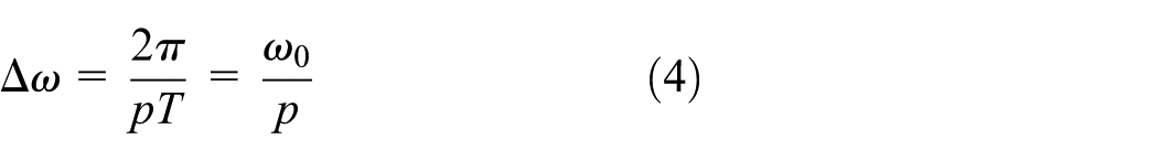
where $ω_{0} = 2 π / T$ .

From equation (4), the Fourier fundamental frequency ( $Δ f$ ) can be defined as

Δ f = \frac{1}{pT} = \frac{1}{p N_{s} T_{s}} = \frac{1}{N T_{s}} = \frac{f_{s}}{N}

(5)

where $N_{s} \overset{Δ}{=} N / p$ and $T_{s} \overset{Δ}{=} 1 / f_{s}$ . Note that the signal is sampled N points using the sampling rate $f_{s}$ .

The waveform power (P) can be expressed using the Parseval relation as^30,31

P = \frac{1}{N} \sum_{n = 0}^{N - 1} i_{s} {[n]}^{2} = \sum_{k = 0}^{N - 1} I_{s} {[k]}^{2}

(6)

At the frequency $f_{k}$ , the power can be expressed as

P [f_{k}] = I_{s} [k]^{2} + I_{s} [N - k]^{2} = 2 I_{s} [k]^{2}

(7)

where k = 0,1, 2, …, N/2 − 1.

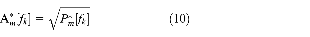
The amplitude of the mth harmonic at $f_{k}$ is thus calculated as

A_{m} [f_{k}] = \sqrt{P [f_{k}]} = \sqrt{2} I_{s} [k]

(8)

where m = 1, 2, …, M.

When the sampling window is not synchronized with the fundamental, the mth harmonic power at $f_{k}$ will disperse over around the $f_{k}$ . Based on the concept of group harmonics, all spilled power around the adjacent harmonics can be collected into a “group power” as^32,33

P_{m}^{*} [f_{k}] = \sum_{Δ k = - τ}^{+ τ} (A_{m} [f_{k + Δ k}])^{2}

(9)

where $τ$ denotes the group bandwidth.

Therefore, the true harmonic amplitude can be retrieved from collecting all dispersed power as

A_{m}^{*} [f_{k}] = \sqrt{P_{m}^{*} [f_{k}]}

(10)

The proposed enhanced FFT algorithm

The proposed enhanced fast Fourier transform (e-FFT) algorithm is to improve the FFT for suiting non-stationary vibration signal measurement. According to the empirical observation from FFT analysis, the relationship between harmonic frequency and dispersed energy can be classified into small-frequency deviation and big-frequency deviation, illustrated as follows.³⁴ Case 1 for small-frequency deviation is shown in Figure 1(a); it indicates that the second larger magnitude ( $A_{m} [f_{k + 1}]$ ) at $f_{k + 1}$ is located at the right side of the dominant frequency at $f_{k}$ , where $A_{m} [f_{k}] > A_{m} [f_{k + 1}]$ . In practice, however, $f_{k}$ may be wrongly interpreted as the dominant harmonic frequency. In a real circumstance, the true frequency is found to be equal to $f_{k}$ plus the “frequency deviation” ( $Δ f_{k}$ ) defined in equation (11). It is also found that higher $A_{m} [f_{k + 1}]$ will introduce more amount of deviation ( $Δ f_{k}$ ) distant from $f_{k}$ . Case 2 for a big-frequency deviation is shown in Figure 1(b); it reveals the situation that the second larger amplitude ( $A_{m} [f_{k}]$ ) at $f_{k}$ is located at the left side of the dominant frequency at $f_{k + 1}$ , where $A_{m} [f_{k}] < A_{m} [f_{k + 1}]$ . The $f_{k + 1}$ can be wrongly interpreted as the dominant harmonic frequency in such a case. Similarly, the true frequency should be equal to $f_{k}$ plus the “frequency deviation” ( $Δ f_{k}$ ). Higher $A_{m} [f_{k + 1}]$ will also introduce more amount of deviation ( $Δ f_{k}$ ) distant from $f_{k}$ . Note that the small- and big-frequency deviations for case 1 and case 2 are defined in the proposed model based on the generic phenomenon of frequency deviation condition. From this principle, the “small” and “big” only denote the deviation situation or margin rather than a real value.

Figure 1.

Relation between harmonic frequency and dispersed energy: (a) small-frequency deviation and (b) big-frequency deviation.³⁴

From the above principle, a mathematical model can be deduced from the relation between the frequency deviation amount and dispersed energy distribution.³⁵ It concludes that the real frequency can be represented by the dominant frequency ( $f_{k}$ ) plus “frequency deviation” ( $Δ f_{k}$ ), that is, $f_{k} + Δ f_{k}$ .

The frequency deviation range (FDR) is therefore defined as³⁵

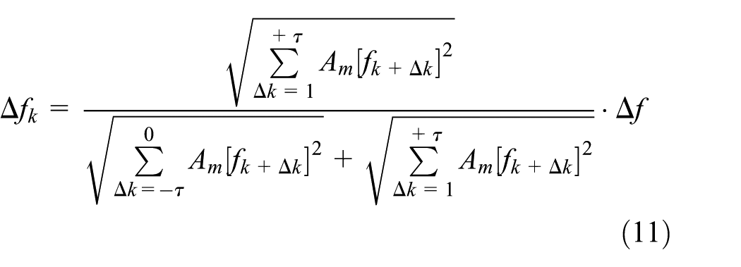
Δ f_{k} = \frac{\sqrt{\sum_{Δ k = 1}^{+ τ} A_{m} {[f_{k + Δ k}]}^{2}}}{\sqrt{\sum_{Δ k = - τ}^{0} A_{m} {[f_{k + Δ k}]}^{2}} + \sqrt{\sum_{Δ k = 1}^{+ τ} A_{m} {[f_{k + Δ k}]}^{2}}} \cdot Δ f

(11)

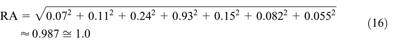
where $Δ f$ is determined by N and $f_{s}$ due to $Δ f = f_{s} / N$ , and $τ = 0, 1, 2, 3, \dots$

On the basis of the group-harmonic concept, the collected energy dispersed around the major harmonic can be used for retrieving the original amplitude. Thus, the restored amplitude (RA) can be defined as³⁵

RA = \sqrt{\sum_{Δ k = - τ}^{+ τ} A_{m} {[f_{k + Δ k}]}^{2}}

(12)

where $τ = 0, 1, 2, 3, \dots$

The following case is demonstrated for more understanding the idea for the definition of both $Δ f$ and RA. Assume the signal, that is, $v (t) = 0.3 \sin (2 π \cdot 670 \cdot t) + 1.0 \sin (2 π \cdot 3180 \cdot t)$ , contains two major vibration signal frequencies located at 670 and 1250 Hz, and their amplitudes are set as 0.3 and 1, respectively. Please note that $f_{s} = 12.8 kHz$ , N = 128, and $τ = 3$ , where $Δ f = 100 Hz$ . The waveform and its spectrum using FFT are shown in Figure 2(a) and (b), respectively. It is clear to see some energy dispersed around the neighbor sides at both 700 and 3200 Hz significantly so that FFT is unable to calculate the spectrum accurately because the signal is not stationary.

Figure 2.

$v (t)$ spectrum using FFT: (a) waveform and (b) spectrum.

At 670 Hz, the FDR beyond 600 Hz can be calculated using equation (11) as

\begin{matrix} Δ f_{k} & = \frac{\sqrt{{0.24}^{2} + {0.045}^{2} + {0.02}^{2} + {0.012}^{2}}}{\sqrt{{0.046}^{2} + {0.062}^{2} + {0.13}^{2}} + \sqrt{{0.24}^{2} + {0.045}^{2} + {0.02}^{2} + {0.012}^{2}}} \cdot Δ f \\ = \frac{0.25}{0.14 + 0.25} \cdot 100 \approx 64.1 Hz \end{matrix}

(13)

\begin{matrix} RA & = \sqrt{{0.046}^{2} + {0.062}^{2} + {0.13}^{2} + {0.24}^{2} + {0.045}^{2} + {0.02}^{2} + {0.012}^{2}} \\ \approx 0.29 ≅ 0.3 \end{matrix}

(14)

This vibration frequency (664 Hz) is found equal to 600 Hz ( $f_{k}$ ) plus 64 Hz ( $Δ f_{k}$ ), very close to the actual frequency value (670 Hz).

At 3180 Hz, the FDR beyond 3100 Hz can be calculated using equation (11) as

\begin{matrix} Δ f_{k} & = \frac{\sqrt{{0.93}^{2} + {0.15}^{2} + {0.082}^{2} + {0.055}^{2}}}{\sqrt{0.0 7^{2} + {0.11}^{2} + {0.24}^{2}} + \sqrt{{0.93}^{2} + {0.15}^{2} + {0.082}^{2} + {0.055}^{2}}} \cdot Δ f \\ = \frac{0.95}{0.27 + 0.95} \cdot 100 \approx 77.89 ≅ 78 Hz \end{matrix}

(15)

\begin{matrix} RA & = \sqrt{0.0 7^{2} + {0.11}^{2} + {0.24}^{2} + {0.93}^{2} + {0.15}^{2} + {0.082}^{2} + {0.055}^{2}} \\ \approx 0.987 ≅ 1.0 \end{matrix}

(16)

This vibration frequency (3178 Hz) is found equal to 3100 Hz ( $f_{k}$ ) plus 78 Hz ( $Δ f_{k}$ ), very close to the actual frequency value (3180 Hz).

The $f_{1}$ and $f_{2}$ are assumed as two arbitrary near major harmonics, where the amplitude of $f_{1}$ is bigger than the $f_{2}$ . If only one major component exits, $f_{2}$ is set as zero. The selection of the group bandwidth ( $τ$ ) is determined by the following rule

\begin{matrix} | f_{1} - f_{2} | < 4 Δ f \Rightarrow τ = 1 \\ 4 Δ f \leq | f_{1} - f_{2} | < 6 Δ f \Rightarrow τ = 2 \\ 6 Δ f \leq | f_{1} - f_{2} | < 8 Δ f \Rightarrow τ = 3 \\ 8 Δ f \leq | f_{1} - f_{2} | < 10 Δ f \Rightarrow τ = 4 \\ | f_{1} - f_{2} | \geq 10 Δ f \Rightarrow τ = 5 \end{matrix}

As stated above, the rule for the selection of the group bandwidth ( $τ = 1 - 5$ ) is determined by the distance between two close harmonics locations to avoid overlapping of each other. This principle is developed based on the empirical observation from FFT analysis.

The flowchart of the proposed e-FFT model is shown in Figure 3, and its implementation procedure is illustrated as follows. Note that the purpose of Figure 3 is to find the FDR and RA for vibration signal spectrum in different locations. Accordingly, the major spectrums of vibration signal can be obtained accurately:

Determine $f_{s}, N$ and sample the signal.

Implement FFT.

Determine the number (M) of major harmonics.

Define the biggest amplitude and second big amplitude at $f_{1}$ and $f_{2}$ , respectively.

Check whether $| f_{1} - f_{2} | < 4 Δ f$ . If yes, select $τ = 1$ and go to Step 10. Otherwise, go to next step.

Check whether $4 Δ f \leq | f_{1} - f_{2} | < 6 Δ f$ . If yes, select $τ = 2$ and go to Step 10. Otherwise, go to next step.

Check whether $6 Δ f \leq | f_{1} - f_{2} | < 8 Δ f$ . If yes, select $τ = 3$ and go to Step 10. Otherwise, go to next step.

Check whether $8 Δ f \leq | f_{1} - f_{2} | < 10 Δ f$ . If yes, select $τ = 4$ and go to Step 10. Otherwise, go to next step.

Select $τ = 5$ .

Calculate $Δ f_{k}$ , RA.

Exclude the $f_{1}$ component (the biggest amplitude) that has been identified, and M = M − 1.

Check whether M = 0. If yes, the procedure stops. Otherwise, go back to Step 4.

Figure 3.

Flowchart of the proposed e-FFT model.

Experimental results

Measurement calibration setup

For the purpose of measurement calibration, the proposed e-FFT model is first performed using known quantity of hardware signals generated from the function generator. The calibration platform setup is shown in Figure 4, but the drilling machine is substituted with the function generator. This calibration ensures that the model can be applied to any practical vibration signal analysis without the loss of measurement precision:

Function generator. It can generate sine and square waveforms to calibrate the measurement result.

Accelerometer amplifier circuit. In Figure 5, the accelerometer amplifier circuit using accelerometer (PCB352A25/NC) is designed to detect and amplify the vibration signal. It mainly consists of four parts: Part A—buffer circuit: it provides a high-input impedance so that the signal from the accelerometer can be read without loss. Note that DC of 18 V with current regulative diode (CRD) is required to activate the accelerometer. Part B—amplification circuit: it can amplify the detected signal of accelerometer with magnification factor = 158. Part C—clamp circuit: it magnifies the signal 6.8 times but limits the output signal within the 5 V range. Part D—second-order filter: it can filter out the undesired noise signal and allow only 0.6–6 k(Hz) signals to pass through the circuit.

Microprocessor (PIC18F4520) with e-FFT model. It is mainly used as the signal-processing tool to implement e-FFT algorithm. The function also includes signal receiving/transmission from/to the Function Generator and the Computer (Data Acquisition and Display System) via RS232/RS485.

Data Acquisition System. The system based on LabVIEW package can receive the data (real-time results from e-FFT model) from the microprocessor and then transmit it to the Data Server immediately. Therefore, the data can be thus read from the Data Server and be displayed on the computer instantly.

Data Server. The MySQL database is used to receive the data from the Data Acquisition System.

Figure 4.

Performance platform.

Figure 5.

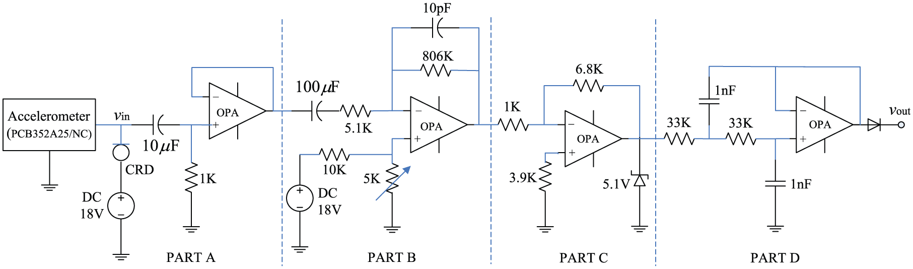
Accelerometer amplifier circuit.

The parameters of e-FFT model are set as f_s = 12.8 kHz and N = 128, that is, $Δ f = 100 Hz$ , for the model performances presented in this section. In this case, the sampling time ( $N \times 1 / f_{s} = 1 / Δ f$ ) is equal to 0.1 s so that it is sufficient to catch up with slight random of the bearing fault signal in practice.

Experimental platform setup

The experimental platform is set up as shown in Figure 4, where the drilling machine is the vibration source using 1 hp alternating current (AC) of 110 V motor with 1730 r/min.

Measurement calibration results

To calibrate the measurement, two known waveforms, that is, sine and triangle waveforms, generated from the Function Generator are employed for test, where both low and high frequencies, that is, 440 Hz and 2.06 kHz, are considered. Please note that every waveform is magnified 1074 times from accelerometer amplifier circuit, and the vibration strength, that is, the spectrum, is presented with the unit “g” (acceleration of gravity) according to the 2.5 mV/g conversion relation from the accelerometer (PCB352A25/NC) datasheet. The $f_{\sin} / a_{\sin}$ and f_square/a_square denote the fundamental frequencies/amplitudes for sine and square waveforms, respectively:

1. Sine waveform at $f_{\sin} = 440 Hz$ and $a_{\sin} = 0.18 g$

In this case, the sine waveform with $f_{\sin} = 440 Hz$ and $a_{\sin} = 0.18 g$ is shown in Figure 6(a), where the peak amplitude is 1.05 V. In Figure 6(b), the frequency and amplitude obtained from FFT are found as $f_{\sin} = 400 Hz$ and $a_{\sin} = 0.13 g$ , respectively. Obviously, the spectrum has a considerable spectral leakage so that a big error occurs. However, the spectrum analysis using e-FFT achieves an accurate outcome, that is, f_sin = 440 Hz and a_sin = 0.17g, almost equal to the real values, as shown in Figure 6(c).

2. Sine waveform at f_sin = 2.06 kHz and a_sin = 0.18g

The sine waveform with f_sin = 2.06 kHz and a_sin = 0.18g is shown in Figure 7(a), where the peak amplitude is 1.04 V. The spectrum using FFT is obtained as f_sin = 2.1 kHz and a_sin = 0.15g, as shown in Figure 7(b). Similarly, the result has a significant error due to the serious leakage problem. In Figure 7(c), the spectrum using e-FFT reaches a highly precise measurement outcome, that is, f_sin = 2.07 kHz and a_sin = 0.18g, almost same as the real values.

3. Square waveform at f_square = 440 Hz and a_square = 0.24g

The square waveform with f_square = 440 Hz and a_square = 0.24g is shown in Figure 8(a), where the peak amplitude is 1.11 V. The spectrum using FFT is obtained as f_square = 400 Hz and a_square = 0.19g, as shown in Figure 8(b). It can be seen that the leakage spreads around the major components so that it causes some significant errors. In Figure 8(c), the spectrum from e-FFT analysis achieves an accurate result, that is, f_square = 440 Hz and a_square = 0.24g for the fundamental component, exactly equal to the real values. The other components also have similar results.

4. Square waveform at f_square = 2.06 kHz and a_square = 0.24g

The square waveform with f_square = 2.06 kHz and a_square = 0.24g is shown in Figure 9(a), where the peak amplitude is 1.13 V. The spectrum using FFT is obtained as f_square = 2.1 kHz and a_square = 0.21g, as shown in Figure 9(b). It is found that the leakage spreading around the fundamental component is evident. Therefore, both f_square and a_square cannot reach a correct outcome. In Figure 9(c), clearly the spectrum analysis using e-FFT accomplishes a quite satisfactory measurement, that is, f_square = 2.07 kHz and a_square = 0.24g, almost same as the real values.

Figure 6.

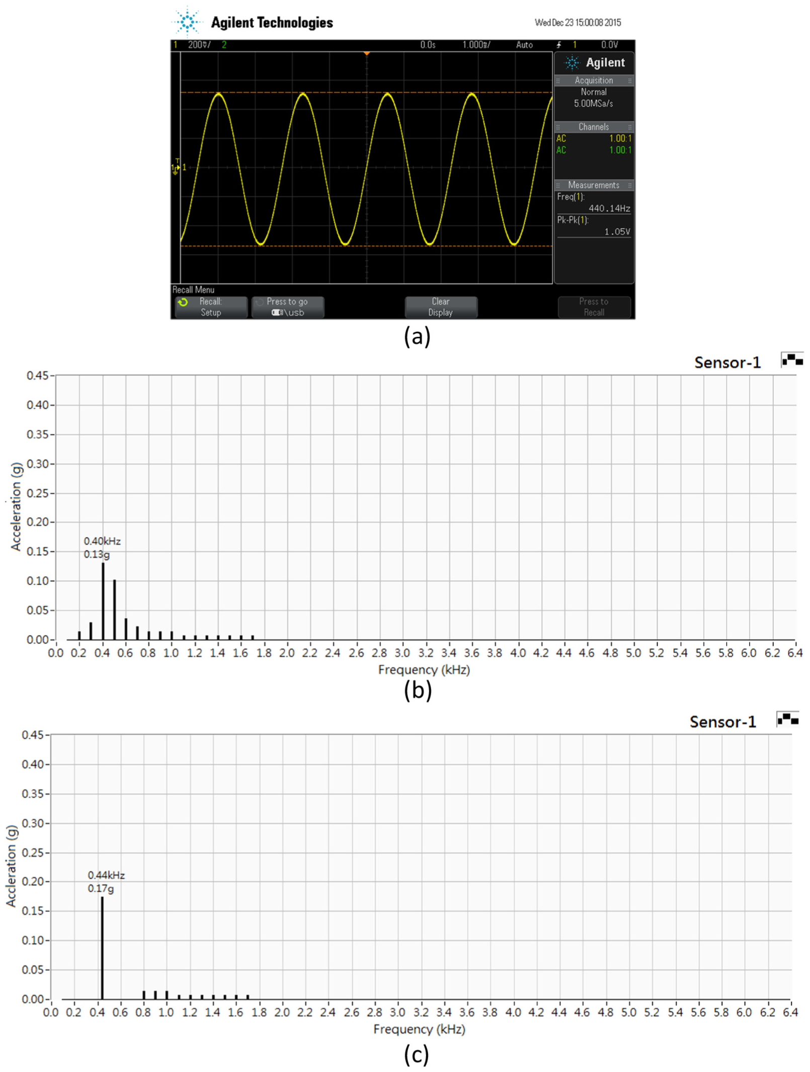
Signal analysis using sine waveform at 440 Hz: (a) sine waveform, (b) spectrum with FFT, and (c) spectrum with e-FFT.

Figure 7.

Signal analysis using sine waveform at 2.06 kHz: (a) sine waveform, (b) spectrum with FFT, and (c) spectrum with e-FFT.

Figure 8.

Signal analysis using square waveform at 440 Hz: (a) square waveform, (b) spectrum with FFT, and (c) spectrum with e-FFT.

Figure 9.

Signal analysis using square waveform at 2.06 kHz: (a) square waveform, (b) spectrum with FFT, and (c) spectrum with e-FFT.

The comparison between FFT and e-FFT is concluded in Table 1. We see that the results from e-FFT model are almost identical to the real values, but traditional FFT is unable to achieve a correct analysis.

Table 1.

Comparison between FFT and e-FFT.

Methods	Waveforms
Methods	Sine waveform		Square waveform
	f _sin = 440 Hz	f _sin = 2.06 kHz	f_square = 440 Hz	f_square = 2.06 kHz
	a _sin = 0.18g	a _sin = 0.18g	a_square = 0.24g	a_square = 0.24g
FFT	f _sin = 400	f _sin = 2.10 k	f_square = 400	f_square = 2.10 k
FFT	a _sin = 0.13	a _sin = 0.15	a_square = 0.19	a_square = 0.21
e-FFT	f _sin = 440	f _sin = 2.07 k	f_square = 440	f_square = 2.07 k
e-FFT	a _sin = 0.17	a _sin = 0.18	a_square = 0.24	a_square = 0.24

FFT: fast Fourier transform; e-FFT: enhanced fast Fourier transform.

Online practical measurement results

To verify the effectiveness of the proposed model for online measurement, the bearing of drilling machine is used as the major vibration source, as shown in Figure 4, where the vibration signal is acquired and analyzed using FFT and e-FFT for comparison. Also, the accelerometer mounting is placed at the surface of bearing near the cutter for testing. Two cases with the small- and big-size cutters were considered for test, which is given as follows:

1. Performance results for drilling machine using small-size cutter

The vibration spectrum (acceleration of gravity) analysis using small-bore cutter is shown in Figure 10. The waveform is shown in Figure 10(a), and its peak amplitude is 1.73 V. The results from FFT and e-FFT measurement are shown in Figure 10(b) and (c), respectively. With FFT, it is seen that the spectrum spreads widely and disorderly. More importantly, there are two major frequencies found being located at 200 and 300 Hz with a low amplitude below 0.05g. However, the e-FFT model has recovered its actual spectrum components more effectively, where the major component is obtained as 260 Hz with 0.05g.

2. Performance results for drilling machine using big-size cutter

The vibration spectrum analysis using big-bore cutter is shown in Figure 11. The waveform is shown in Figure 11(a). Its peak amplitude as 4.66 V implies that the vibration strength is much higher than the case using small-size cutter. The results from FFT and e-FFT measurement are shown in Figure 11(b) and (c), respectively. With FFT, there are totally five major spectrum components beyond 0.05g at different locations. The frequencies are found as 0.90, 1.00, 3.40, 3.70, and 3.80 kHz, and their amplitudes are 0.05g, 0.09g, 0.06g, 0.05g, and 0.07g, respectively. Contrastively, the e-FFT model has successfully regained its major spectrum frequencies as 0.96, 3.36, and 3.76 kHz with respective amplitudes as 0.10, 0.07, and 0.08 g. Obviously, this outcome reveals that only three strong vibration components appear in the vibration signal in reality.

Figure 10.

Vibration spectrum analysis using small-bore cutter: (a) vibration waveform, (b) spectrum with FFT, and (c) spectrum with e-FFT.

Figure 11.

Vibration spectrum analysis using big-bore cutter: (a) vibration waveform, (b) spectrum with FFT, and (c) spectrum with e-FFT.

Observation determination of group bandwidth ( $τ$ ), sampled point (N), and sampling rate (f_s)

The group bandwidth ( $τ$ ) plays a crucial role in the proposed approach and it should be chosen appropriately. The larger group bandwidth ( $τ$ ) may collect all dispersed power and thus regain the actual amplitude more accurately. However, a large $τ$ may lead to a dispersed power overlap within near major vibration harmonics. Consequently, $τ$ should be chosen as large as possible but small enough to avoid the overlap between two neighboring vibration harmonics. In this study, the selection rule of $τ$ (1–5) has been formulated, depending on the distribution situation of dispersed energy.

It is also important to note that the N can be extended to $N = 2^{m}$ , for example, 64, 128, 256, 512, 1024, …, using f_s = 12.8 kHz, where $Δ f = 200, 100, 50, 25, 12.5, \dots$ , respectively. Correspondingly, the sampling time will be 5, 10, 20, and 40 ms, …, respectively. As can be seen, an increasing N can obtain lower $Δ f$ to achieve higher resolution, but it will pay for longer sampling time. Hence, both $Δ f$ and sampling time should come to a compromise, particularly for the instantaneous rate of vibration change to be taken account.

Conclusion

The vibration status caused from rolling-element bearings is a critical health condition of the rotating machinery. Currently, many techniques such as FFT, STFT, and CWT have been reported for time–frequency analysis. However, they may still suffer from less efficiency in analyzing non-stationary signals produced from the rolling machine. The proposed e-FFT model can collect dispersed energy and thus recover its original amplitude effectively. Also, the frequency can be regained using a simple arithmetic computation accurately. Before practical analysis, the model was calibrated with known sine and triangle waveforms to verify its reliability and precision. The group bandwidth ( $τ$ ) is determined between 1 and 5 according to the selection rule of the e-FFT so that it can reach the most correct solution. Based on $Δ f = 100$ , the sampling time for acquiring vibration signal takes only 0.01 s so that it can react to rapid change of machine vibration. As can be seen from Table 1, it is evident that the e-FFT model is superior to traditional FFT. Additionally, if the machine is involved in different vibration sources, the influence between each other may not be avoided. For example, it may result in several sideband frequencies due to the effect of linear superposition and nonlinear effects from additional machine vibrations. This problem becomes too complex to be resolved easily by current techniques, particularly in the isolation and diagnosis of the complex bearing signals. Therefore, it is worthy to work out for the future research work.

Footnotes

Academic Editor: Balla Prasad

Declaration of conflicting interests

The author(s) declared no potential conflicts of interest with respect to the research, authorship, and/or publication of this article.

Funding

The author(s) received no financial support for the research, authorship, and/or publication of this article.

References

Lacey

SJ.

An overview of bearing vibration analysis. Mainten Asset Manag 2008; 23: 32–42.

Zhu

. Investigation on full ceramic bearing fault diagnostics using vibration and AE sensors. In: 2012 IEEE conference on prognostics and health management, Colorado, USA, 18–21 June 2012, pp.1–2. New York: IEEE.

Pan

Tsao

Using appropriate IMFs for envelope analysis in multiple fault diagnosis of ball bearings. Int J Mech Sci 2013; 69: 114–124.

Slavic

Brkovic

Boltezar

Typical bearing-fault rating using force measurements-application to real data. J Vib Control 2012; 17: 2164–2174.

Randall

Antoni

Rolling element bearing diagnostics. Mech Syst Signal Pr 2011; 25: 485–520.

Aherwar

Saifullah Khalid

Vibration analysis techniques for gearbox diagnostic: a review. Int J Adv Sci Eng Tech 2012; 3: 4–12.

Fan

A hybrid approach for fault diagnosis of planetary bearings using an internal vibration sensor. Measurement 2015; 64: 71–80.

Milan Singh

Sumathi

. Vibration parameter estimation methods for ultrasonic measurement systems—a review. IET Sci Measurement Technol 2015; 9: 492–504.

Lee

D -H

Lee

Ahn

J -W.

Mechanical vibration reduction control of two-mass permanent magnet synchronous motor using adaptive notch filter with fast Fourier transform analysis. IET Electr Power Appl 2012; 6: 455–461.

10.

Rui

Wang

Zhu

. Vibration characteristics of various surfaces using an LDV for long-range voice acquisition. IEEE Sens J 2011; 11: 1415–1422.

11.

Singleton

Strangas

Aviyente

Extended Kalman filtering for remaining-useful-life estimation of bearings. IEEE T Ind Electron 2015; 62: 1781–1790.

12.

Study on fault detection of rolling element bearing based on translation-invariant denoising and Hilbert-Huang transform. J Comp 2012; 7: 1142–1146.

13.

Saxena

Chowdhury

Devendiran

Assessment of gearbox fault detection using vibration signal analysis and acoustic emission technique. J Mech Civ Eng 2013; 7: 52–60.

14.

Bhende

Awari

Untawale

Assessment of bearing fault detection using vibration signal analysis. J Tech Non-Tech 2011; 2: 249–261.

15.

Rai

Mohanty

AR.

Bearing fault diagnosis using FFT of intrinsic mode functions in Hilbert–Huang transform. Mech Syst Signal Pr 2007; 21: 2607–2615.

16.

Atoui

Meradi

Boulkroune

. Fault detection and diagnosis in rotating machinery by vibration monitoring using FFT and Wavelet techniques. In: 2013 8th international workshop on systems, signal processing and their applications (WoSSPA), Algiers, Algeria, 12–15 May 2013, pp.401–406. New York: IEEE.

17.

Patil

Gaikwad

. Vibration analysis of electrical rotating machines using FFT: a method of predictive maintenance. In: 2013 fourth international conference on computing, communications and networking technologies (ICCCNT), Tiruchengode, India, 4–6 July 2013, pp.1–6. New York: IEEE.

18.

Qin

Chen

Bao

Continuous wavelet transform for nonstationary vibration detection with phase-OTDR. Opt Express 2012; 20: 20459–20465.

19.

Satish

Short-time Fourier and wavelet transform for fault detection in power transformers during impulse tests. IEE Proc Sci Meas Tech 1998; 145: 77–84.

20.

Gao

Yan

Non-stationary signal processing for bearing health monitoring. Int J Manuf Res 2006; 1: 18–40.

21.

Staszewski

Worden

Tomlinson

GR.

Time-frequency analysis in gearbox fault detection using the Wigner-Ville distribution and pattern recognition. Mech Syst Signal Pr 1997; 11: 673–692.

22.

Baydar

Ball

Detection of gear failures via vibration and acoustic signals using wavelet transform. Mech Syst Signal Pr 2003; 17: 787–804.

23.

Sifuzzaman

Islam

Ali

MZ.

Application of wavelet transform and its advantages compared to Fourier transform. J Phys Sci 2009; 13: 121–134.

24.

Bendjama

Bouhouche

Boucherit

MS.

Application of wavelet transform for fault diagnosis in rotating machinery. Int J Mach Lear Comp 2012; 2: 82–87.

25.

Bendjama

Bouhouche

Moussaoui

. Wavelet transform for bearing faults diagnosis. In: Proceedings of the 2013 conference of advances in control engineering, Istanbul, Turkey, 5–7 September 2013, pp.85–88. Scientific Cooperations.

26.

Djebala

Ouelaa

Benchaabane

. Application of the Wavelet Multi-resolution Analysis and Hilbert transform for the prediction of gear tooth defects. Meccanica 2012; 47: 1601–1612.

27.

Zhang

Zheng

Hilbert-Huang transform and marginal spectrum for detection and diagnosis of localized defects in roller bearings. J Mech Sci Technol 2009; 23: 291–301.

28.

Yan

Gao

RX.

Hilbert–Huang transform-based vibration signal analysis for machine health monitoring. IEEE T Instrum Meas 2006; 55: 2320–2329.

29.

Feldman

Hilbert transform in vibration analysis. Mech Syst Signal Pr 2011; 25: 735–802.

30.

Oppenheim

Schafer

RW.

Discrete-time signal processing. Upper Saddle River, NJ: Prentice Hall, 1989.

31.

Press

Flannery

Teukolsky

. Numerical recipes-The art of scientific computing. Cambridge: Cambridge University Press, 1986, pp.420–429.

32.

IEC 61000–4–7: 2002. Electromagnetic compatibility (EMC) Part 4: testing and measurement techniques Section 7: general guide on harmonics and interharmonics measurements and instrumentation for power supply systems and equipment connected thereto.

33.

Hanzelka

Bien

Power quality application guide. Kraków: AGH University of Science and Technology, 2004.

34.

Lin

HC.

Separation of adjacent interharmonics using maximum energy retrieving algorithm. IET Sci Measurement Technol 2016; 10: 92–99.

35.

Lin

HC.

Development of leakage energy allocation approach for time-varying interharmonics tracking. IET Gener Transm Distrib 2015; 9: 798–804.