Analytical evaluation of geometric dilution of precision for three-dimensional angle-of-arrival target localization in wireless sensor networks

Abstract

This article focuses on the evaluation of geometric dilution of precision for three-dimensional angle-of-arrival target localization in wireless sensor networks. We calculate a general analytical expression for the geometric dilution of precision for three-dimensional angle-of-arrival target localization. Unlike the existing works in the literature, in this article, no assumptions are made regarding the observation ranges, noise variances, or the number of sensors in the derivation of the geometric dilution of precision. Necessary and sufficient conditions regarding the existence of geometric dilution of precision are also derived, which can be readily used to evaluate the observability of three-dimensional angle-of-arrival target localization in wireless sensor networks. Moreover, a concise procedure is also presented to calculate the geometric dilution of precision when it exists. Finally, several examples are used to illustrate our results, and it is shown that the performance of the proposed regular deployment configurations of angle-of-arrival sensors is better than the one with random deployment patterns.

Introduction

Target localization plays an important role for many applications in both military and civilian fields. ¹ A typical application is the global navigation satellite system (GNSS), which can provide autonomous geo-spatial positioning with global coverage and allow small electronic receivers to obtain their locations to high precision using time signals transmitted along a line-of-sight (LOS) by radio from satellites.^2,3 Another emerging application is indoor target localization. To promote market adoption for indoor localization systems, the definition of benchmarking methodologies, common evaluation criteria, standardized methodologies useful to developers, testers, and end users was first proposed, ⁴ and then an attempt to define what is next for indoor localization systems was also performed. ⁵ For indoor and outdoor target localization, the most popular topics of target localization are all involved in the performance measure of accuracy and the corresponding localization algorithm. In this article, we are only interested in the performance measure for three-dimensional (3D) passive target localization using angle-of-arrival (AOA) sensors via a wireless sensor network (WSN).

The most used performance measures of target localization are the geometric dilution of precision (GDOP), ⁶ the Cramér–Rao lower bound (CRLB), ⁷ and the root mean squared (RMS) error.^8,9 In many practical applications, the GDOP plays an important role for evaluating the accuracy of target localization for both two-dimensional (2D) and 3D scenarios. The concept of GDOP is first defined as the ratio of the RMS position error to the RMS ranging error, ⁶ and subsequently, many researchers adopt RMS position error as GDOP directly.^10–12 Actually, as pointed out by Zhong et al., ¹² there are no essential differences between the above-mentioned two definitions. GDOP can be derived from CRLB (if it exists), while CRLB is the inverse of the Fisher information matrix (FIM) and also is the lower bound of any estimation error covariance matrix, ⁹ which, however, can be attained by using any unbiased estimators.

In this article, we adopt the second definition of GDOP, i.e., it is defined as the trace of the CRLB. GDOP shows how the localization accuracy is affected by the sensor-target geometry and can be used to evaluate the final localization estimation. ¹³ The specific style of GDOP for characterizing the performance measure of target localization depends primarily on the adoption of specific sensors. In WSNs, the most frequently used sensors for target localization include range-only sensors, ¹⁴ AOA-based sensors,^15–17 time-difference-of-arrival (TDOA)-based sensors, frequency-difference-of-arrival-based sensors, ¹⁸ and so on. Since GDOP can be used to characterize the target estimate’s uncertainty, many researchers are dedicated to deriving the analytical formulas of GDOP for target localization with the above-mentioned sensors used in some specific application scenarios.^19–27

Until now, most of the existing works have been concentrated on the derivation of analytical formulas of GDOP for 2D case.^{20–23,28,29} Indeed, there exist many application scenarios which are inherently involved in 3D space. For example, the following application scenarios, the determination of user’s location in the GNSS and the aerial target localization and tracking, are all involved in 3D. For 3D space, with the increase in the dimension of the FIM or CRLB, the derivation of GDOP for the arbitrary number of sensors becomes more challenging. To handle this problem, many works have been devoted to deriving the CRLB for the evaluation of 3D AOA target localization.^{16,17,27,30–32} Zhong et al. ¹² propose an analytical formula of GDOP for 3D bearings-only passive target localization. However, an additional assumption on the observation noise variances is needed. Huang et al. ¹⁶ derive the CRLB for the AOA-assisted GNSS collaborative positioning in order to fuse information from GNSS satellites and terrestrial wireless systems. Shim et al. ¹⁷ investigate the CRLB on AOA estimation of an RF lens–embedded antenna array and confirm that the CRLB of an RF lens–embedded antenna array may be better than the CRLB for a conventional uniform linear array in a certain desired range. Xu and Doğançay ³³ derive the formula of the FIM for 3D AOA target localization, then use it to solve the problem of optimal sensor–target geometries. The formula of CRLB for positioning with both range and AOA measurements in a 3D environment is derived by Yu, ²⁶ where the CRLB is used to evaluate positioning accuracy under realistic conditions. The theoretical limit of AOA for cooperative vehicle-to-vehicle scenario is considered in Youn et al., ²⁷ where the theoretical limit is represented as CRLB. Noroozi and Sebt ³⁰ propose the algebraic solution for 3D TDOA/AOA localization in multiple-input-multiple-output passive radar, and the corresponding CRLB is also derived. Kazemi et al. ³¹ and Li et al. ³² are, respectively, devoted to finding the closed-form solution of estimators, and using the derived CRLB, the performance of the proposed algorithms can reach or converge to the CRLB. In Rui and Ho ³⁴ and Moreno-Salinas et al., ³⁵ the minimization of the trace of the CRLB (i.e. GDOP) using time-of-arrival sensors and AOA sensors are considered, respectively, for 2D and/or 3D target localization. However, some restrictive assumptions are made which require that either the number of sensors is even or the observation ranges and/or noise variances are identical for the derivation of the CRLB or GDOP. Although many works have been performed on the derivation of CRLB for 3D AOA target localization, however, very few studies in the literature have considered the problem of deriving explicit expressions of GDOP for 3D AOA target localization in general application scenario.

Along with the determination of the formula of the GDOP (CRLB), the existence conditions of GDOP (CRLB) for AOA target localization have also attracted the attention of researchers. For this case, the existence conditions of GDOP are equivalent to the observability conditions for AOA-based target localization. The observability conditions for bearing-only (angles-only) target localization/tracking have been widely studied.^36–39 However, most of the existing works on the observability problem have primarily focused on the scenario where only one single observer (own-ship) is used for localization or to track the target. For multiple 3D AOA sensors case in WSNs, to the best of our knowledge, the observability conditions have been rarely studied.

Motivated by the above discussions, this article is devoted to determining the explicit expression of GDOP as well as the existence conditions of GDOP for 3D AOA target localization in more general application scenarios. First, we derive the FIM for 3D AOA sensors using the measurement likelihood function according to the observation equations of azimuth and elevation angles. Then, rearranging the FIM as a special form, the Cauchy–Binet formula is adopted to derive the analytical formula of GDOP. Finally, the conditions are derived regarding the existence of the GDOP. The main contributions of this article are threefold: (1) a general analytical formula of GDOP with closed form for 3D AOA target localization is proposed, where no restrictive assumptions are needed on the number of sensors, the observation ranges and noise variances; thus, the presented formula of GDOP can be used to evaluate the accuracy of 3D AOA target localization for most general scenarios; (2) some existing works on the GDOP for 2D/3D AOA target localization can be regarded as the special case of the proposed approach, which can be directly deduced from the proposed general analytical formula of GDOP; (3) a necessary and sufficient condition for the invertibility of the FIM for 3D AOA target localization is given, which can be used to judge the existence of GDOP. Moreover, a concise procedure of evaluating the GDOP for 3D AOA target localization is presented.

The remainder of this article is organized as follows. Section “Problem formulation” gives the problem formulation of 3D AOA target localization, and the derivation of the FIM is addressed in section “Derivation of the FIM for 3D AOA sensors.” Section “Derivation of the GDOP for 3D AOA sensors” is dedicated to characterizing the generalized GDOP using explicit expression for 3D AOA target localization. Some special cases of GDOP are studied in section “Special case studies,” and then in section “Illustrative examples” several examples are illustrated and section “Conclusion” concludes the article.

Notations and definitions

The two-norm for a vector of $\mathit{x}\in {\mathbb{R}}^{n_x}$ is defined as $\parallel \mathit{x}\parallel =\parallel \mathit{x}{\parallel }_2=\sqrt{{\mathit{x}}^{\top }\mathit{x}}$ . $〈\mathit{a},\mathit{b}〉$ denotes the inner product between two vectors $\mathit{a}$ and $\mathit{b}$ . $\det (\mathit{A})$ or $|\mathit{A}|$ represents the determinant of the matrix $\mathit{A}$ . $\mathrm{tr}(\mathit{A})$ and ${\mathit{A}}^{\top }$ indicate the trace and transpose of the matrix $\mathit{A}$ , respectively.

Problem formulation

Consider the target localization problem of $n(n\ge 2)$ AOA sensors in 3D space using angle-only observations in WSNs. The sensor-target geometry is shown in Figure 1, where ${\mathit{p}}_t:=[x_t,y_t,z_t{]}^{\top }\in {\mathbb{R}}^3$ and ${\mathit{s}}_i:=[x_i,y_i,z_i{]}^{\top }\in {\mathbb{R}}^3$ are the mutually distinct position vectors of the target and sensor i in the Cartesian coordinate system of Oxyz, respectively, $i\in \{1,2,\dots ,n\}$ . Define ${\mathit{r}}_i={\mathit{p}}_t-{\mathit{s}}_i$ as the vector of LOS from sensor i to the target, then $r_i=\parallel {\mathit{r}}_i\parallel$ represents the distance (range) between the target and sensor i. ${\theta }_{\mathrm{ij}}$ is the angle of LOS between the sensors i and j, and ${\theta }_{\mathrm{ij}}={\theta }_{\mathrm{ji}}\in [0,\pi ]$ . ${\beta }_i$ and ${\alpha }_i$ are the azimuth and elevation angles of LOS of the ith sensor, respectively, defined by

$${\beta }_i=h_{i,1}\left({\mathit{p}}_t\right)={\tan }^{-1}\left(\frac{y_t-y_i}{x_t-x_i}\right)$$

(1)

$${\alpha }_i=h_{i,2}\left({\mathit{p}}_t\right)={\sin }^{-1}\left(\frac{z_t-z_i}{r_i}\right)$$

(2)

where ${\tan }^{-1}(·)$ is the four-quadrant arctangent and ${\sin }^{-1}(·)$ is the arcsine.

Figure 1.

Geometric configuration of the target and sensors.

Remark 1

Note that the use of elevation and azimuth angles in 3D AOA target localization inevitably introduces discontinuities and singularities. ⁴⁰ If $\exists i\in \{1,2,\cdots ,n\}$ , ${\alpha }_i\in \{\pm \pi /2\}$ , then the azimuth ${\beta }_i$ is arbitrary and undefined for 0/0 due to $x_t=x_i$ and $y_t=y_i$ in equation (1). Conventionally, for these special cases, there are two mathematical treatments: ⁴¹ one is that the azimuth ${\beta }_i$ is designated as a fixed constant such as zero to guarantee the uniqueness of coordinates, the other is to restrict the elevation of ${\alpha }_i$ over the interval of $(-\pi /2,\pi /2)$ to avoid the indetermination of ${\beta }_i$ . Since the inherent singularities of the use of azimuth/elevation angular representation, these special cases are usually not considered and directly ignored in the literature.^12,33,35 In this article, we also use the convention of ruling out the singular points ${\alpha }_i=\pm \pi /2$ and adopt the second treatment, and then focus on the problem of evaluating the GDOP for 3D AOA target localization with ${\alpha }_i\in (-\pi /2,\pi /2),{\beta }_i\in (-\pi ,\pi ],\forall i\in \{1,2,\dots ,n\}$ .

In practice, the AOA observations of ${\beta }_i$ and ${\alpha }_i$ can be obtained directly by equipping a directional antenna or antenna array on each sensor. ⁴² Define ${\mathit{z}}_i:=[{\tilde{\beta }}_i,{\tilde{\alpha }}_i{]}^{\top }\in {\mathbb{R}}^2$ as the observation vector of sensor i, where ${\tilde{\beta }}_i$ and ${\tilde{\alpha }}_i$ are designated as the observation values of the true angles of ${\beta }_i$ and ${\alpha }_i$ , respectively, then the observation equation can be written with the compact form

$${\mathit{z}}_i={\mathit{h}}_i\left({\mathit{p}}_t\right)+{\mathit{v}}_i$$

(3)

where ${\mathit{h}}_i({\mathit{p}}_t)=[h_{i,1}({\mathit{p}}_t),h_{i,2}({\mathit{p}}_t){]}^{\top }$ is the observation function vector and ${\mathit{v}}_i\in {\mathbb{R}}^2$ is the observation noise vector. All sensor noises are assumed to be mutually independent and identically distributed Gaussian noise sequences with mean zero and covariance ${\mathit{R}}_i$ , that is, ${\mathit{v}}_i~\mathcal{N}(0,{\mathit{R}}_i),i\in \{1,2,\dots ,n\}$ . Here, ${\mathit{R}}_i$ is given by

$${\mathit{R}}_i=\left[\begin{array}{cc}{\sigma }_{{\beta }_i}^2\hfill & 0\hfill \\ \multicolumn{1}{c}{0}& {\sigma }_{{\alpha }_i}^2\hfill \end{array}\right]$$

(4)

where ${\sigma }_{{\beta }_i}^2$ and ${\sigma }_{{\alpha }_i}^2$ are the observation noise variances of ${\beta }_i$ and ${\alpha }_i$ , respectively. The estimation error covariance matrix of ${\mathit{p}}_t$ is defined by

$$\mathit{P}=\mathcal{E}\left\{({\mathit{p}}_t-{\hat{\mathit{p}}}_t){({\mathit{p}}_t-{\hat{\mathit{p}}}_t)}^{\top }\right\}$$

(5)

where ${\hat{\mathit{p}}}_t$ is the estimate of the target position vector ${\mathit{p}}_t$ . It is well known that the inverse of the FIM (when it exists, called the CRLB) is the lower bound of the covariance matrix $\mathit{P}$ ⁹

$$\mathit{P}\ge {\mathit{J}}^{-1}=\mathrm{CRLB}$$

(6)

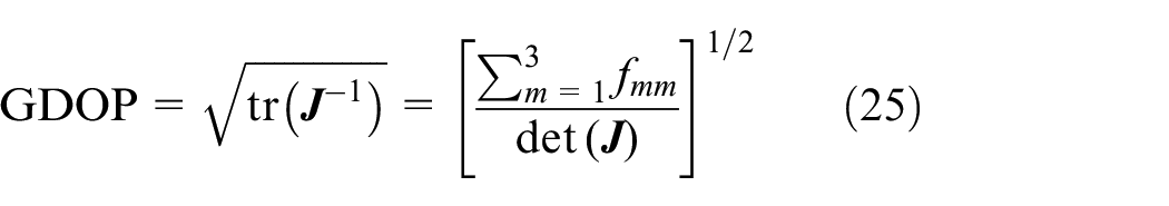
where $\mathit{J}$ is the FIM. Then the GDOP is defined as

$$\mathrm{GDOP}=\sqrt{\mathrm{tr}(\mathrm{CRLB})}$$

(7)

Now the problems are formally defined as below.

Problem 1. For $n\ge 2$ AOA sensors for 3D target localization in Figure 1, determine the necessary and sufficient condition of the invertibility of the FIM.

Problem 2. For $n\ge 2$ AOA sensors for 3D target localization in Figure 1, if the FIM is invertible, determine the analytical explicit expression of GDOP defined in equation (7) with arbitrary observation ranges of $r_i$ and noise variances of ${\sigma }_{{\beta }_i}^2$ and ${\sigma }_{{\alpha }_i}^2$ .

Derivation of the FIM for 3D AOA sensors

Define ${\mathit{z}}_{1:n}\stackrel{\mathrm{\Delta }}{=}\{{\mathit{z}}_i{\}}_{i=1}^n$ , the likelihood function with respect to ${\mathit{p}}_t$ is

$$L\left({\mathit{p}}_t\right)=p({\mathit{z}}_1,{\mathit{z}}_2,\dots ,{\mathit{z}}_n|{\mathit{p}}_t)=p({\mathit{z}}_{1:n}|{\mathit{p}}_t)$$

(8)

where

$$p({\mathit{z}}_{1:n}|{\mathit{p}}_t)=\underset{i=1}{\overset{n}{\Pi }}\frac{1}{2\pi |{\mathit{R}}_i{|}^{1/2}}\exp \{-\frac{1}{2}W\}$$

(9)

with

$$W={[{\mathit{z}}_i-{\mathit{h}}_i\left({\mathit{p}}_t\right)]}^{\top }{\mathit{R}}_i^{-1}[{\mathit{z}}_i-{\mathit{h}}_i\left({\mathit{p}}_t\right)]$$

(10)

Then the FIM is defined by

$$\mathit{J}=\mathcal{E}\left\{\left[{\nabla }_{{\mathit{p}}_t}\ln p({\mathit{z}}_{1:n}|{\mathit{p}}_t)\right]{\left[{\nabla }_{{\mathit{p}}_t}\ln p({\mathit{z}}_{1:n}|{\mathit{p}}_t)\right]}^{\top }\right\}$$

(11)

Note that

$$\ln p({\mathit{z}}_{1:n}|{\mathit{p}}_t)=-\sum _{i=1}^n\{\ln (2\pi |{\mathit{R}}_i{|}^{1/2})+\frac{1}{2}W\}$$

(12)

Thus, we have

$${\nabla }_{{\mathit{p}}_t}\ln p({\mathit{z}}_{1:n}|{\mathit{p}}_t)=\sum _{i=1}^n\left[{\nabla }_{{\mathit{p}}_t}{\mathit{h}}_i^{\top }\left({\mathit{p}}_t\right)\right]{\mathit{R}}_i^{-1}[{\mathit{z}}_i-{\mathit{h}}_i\left({\mathit{p}}_t\right)]$$

(13)

Submitting equation (13) into equation (11) leads to the form of FIM

$$\mathit{J}=\sum _{i=1}^n{\mathit{H}}_i{\mathit{R}}_i^{-1}{\mathit{H}}_i^{\mathrm{T}}$$

(14)

where

$$\begin{array}{c}{\mathit{H}}_i={\nabla }_{{\mathit{p}}_t}{\mathit{h}}_i^{\top }\left({\mathit{p}}_t\right)=\left[\begin{array}{cc}\frac{\partial h_{i,1}\left({\mathit{p}}_t\right)}{\partial x_t}\hfill & \frac{\partial h_{i,2}\left({\mathit{p}}_t\right)}{\partial x_t}\hfill \\ \multicolumn{1}{c}{\frac{\partial h_{i,1}\left({\mathit{p}}_t\right)}{\partial y_t}}& \frac{\partial h_{i,2}\left({\mathit{p}}_t\right)}{\partial y_t}\hfill \\ \multicolumn{1}{c}{\frac{\partial h_{i,1}\left({\mathit{p}}_t\right)}{\partial z_t}}& \frac{\partial h_{i,2}\left({\mathit{p}}_t\right)}{\partial z_t}\hfill \end{array}\right]\hfill \end{array}$$

(15)

Let ${\mathit{D}}_i{\mathit{D}}_i^{\top }={\mathit{R}}_i^{-1}$ , which yields the unique principal (positive definite) solution

$${\mathit{D}}_i=\left[\begin{array}{cc}{({\sigma }_{{\beta }_i})}^{-1}\hfill & 0\hfill \\ \multicolumn{1}{c}{0}& {({\sigma }_{{\alpha }_i})}^{-1}\hfill \end{array}\right]$$

(16)

and then equation (14) can be rewritten as

$$\mathit{J}=\sum _{i=1}^n\left[{\mathit{H}}_i{\mathit{D}}_i\right]{\left[{\mathit{H}}_i{\mathit{D}}_i\right]}^{\top }$$

(17)

where ${\mathit{H}}_i{\mathit{D}}_i$ is denoted as the product of the two matrices ${\mathit{H}}_i$ and ${\mathit{D}}_i$ . Denoting $[{\mathit{H}}_i{\mathit{D}}_i{]}^{\top }$ as ${\mathbf{G}}_i$ with the form of

$${\mathit{G}}_i={\left[{\mathit{H}}_i{\mathit{D}}_i\right]}^{\top }={[{\mathit{a}}_i,{\mathit{b}}_i]}^{\top }$$

(18)

where

$$\{\begin{array}{c}{\mathit{a}}_i=c_i{[-\sin \left({\beta }_i\right),\cos \left({\beta }_i\right),0]}^{\top }\hfill \\ \multicolumn{1}{c}{{\mathit{b}}_i=g_i{[-\sin \left({\alpha }_i\right)\cos \left({\beta }_i\right),-\sin \left({\alpha }_i\right)\sin \left({\beta }_i\right),\cos \left({\alpha }_i\right)]}^{\top }}\end{array}$$

(19)

with

$$c_i={\left[r_i{\sigma }_{{\beta }_i}\cos \left({\alpha }_i\right)\right]}^{-1},g_i={\left[r_i{\sigma }_{{\alpha }_i}\right]}^{-1}$$

(20)

Then the FIM of equation (17) can be formulated as

$$\mathit{J}=\sum _{i=1}^n{\mathit{G}}_i^{\top }{\mathit{G}}_i=\sum _{i=1}^n({\mathit{a}}_i{\mathit{a}}_i^{\top }+{\mathit{b}}_i{\mathit{b}}_i^{\top })=\mathit{F}{\mathit{F}}^{\top }$$

(21)

where

$$\mathit{F}=[{\mathit{G}}_1^{\top },{\mathit{G}}_2^{\top },\dots ,{\mathit{G}}_n^{\top }]=[{\mathit{a}}_1,{\mathit{b}}_1,\dots ,{\mathit{a}}_n,{\mathit{b}}_n]$$

(22)

It is readily observed that the FIM in equation (21) is a positive (semi-)definite matrix.

Derivation of the GDOP for 3D AOA sensors

Recall the definition of GDOP in equation (7). The inverse of FIM (CRLB) should be determined at first for the derivation of GDOP. If the FIM is positive definite or non-singular, then the inverse of $\mathit{J}$ exists, and the CRLB can be written as

$$\mathrm{CRLB}={\mathit{J}}^{-1}=\frac{{\mathit{J}}^{*}}{det(\mathit{J})}$$

(23)

where ${\mathit{J}}^{*}$ is the adjugate of $\mathit{J}$ , denoted as

$${\mathit{J}}^{*}=\left[\begin{array}{ccc}{f}_{11}\hfill & *\hfill & *\hfill \\ \multicolumn{1}{c}{f_{21}}& f_{22}\hfill & *\hfill \\ \multicolumn{1}{c}{f_{31}}& f_{32}\hfill & f_{33}\hfill \end{array}\right]$$

(24)

By the definition of GDOP in equation (7), we have

$$\mathrm{GDOP}=\sqrt{\mathrm{tr}\left({\mathit{J}}^{-1}\right)}={\left[\frac{\sum _{m=1}^3{f}_{\mathrm{mm}}}{det(\mathit{J})}\right]}^{1/2}$$

(25)

The cofactor of $f_{\mathrm{mm}}$ can be determined by the $(m,m)$ minor of $\mathit{J}$

$$f_{\mathrm{mm}}=(-1{)}^{m+m}\det \left({\mathit{J}}_{\mathrm{mm}}\right)=\det \left({\mathit{J}}_{\mathrm{mm}}\right)$$

(26)

where

$${\mathit{J}}_{\mathrm{mm}}={\mathit{F}}_m{\mathit{F}}_m^{\top },{\mathit{F}}_m=[{\mathit{a}}_1^m,{\mathit{b}}_1^m,\dots ,{\mathit{a}}_n^m,{\mathit{b}}_n^m]$$

(27)

and

$$\{\begin{array}{c}{\mathit{a}}_i^1=c_i{[\cos \left({\beta }_i\right),0]}^{\top }\hfill \\ \multicolumn{1}{c}{{\mathit{b}}_i^1=g_i{[-\sin \left({\alpha }_i\right)\sin \left({\beta }_i\right),\cos \left({\alpha }_i\right)]}^{\top }}\\ \multicolumn{1}{c}{{\mathit{a}}_i^2=c_i{[-\sin \left({\beta }_i\right),0]}^{\top }}\\ \multicolumn{1}{c}{{\mathit{b}}_i^2=g_i{[-\sin \left({\alpha }_i\right)\cos \left({\beta }_i\right),\cos \left({\alpha }_i\right)]}^{\top }}\\ \multicolumn{1}{c}{{\mathit{a}}_i^3=c_i{[-\sin \left({\beta }_i\right),\cos \left({\beta }_i\right)]}^{\top }}\\ \multicolumn{1}{c}{{\mathit{b}}_i^3=g_i{[-\sin \left({\alpha }_i\right)\cos \left({\beta }_i\right),-\sin \left({\alpha }_i\right)\sin \left({\beta }_i\right)]}^{\top }}\end{array}$$

(28)

Calculation of the determinant of the FIM

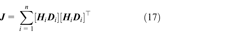
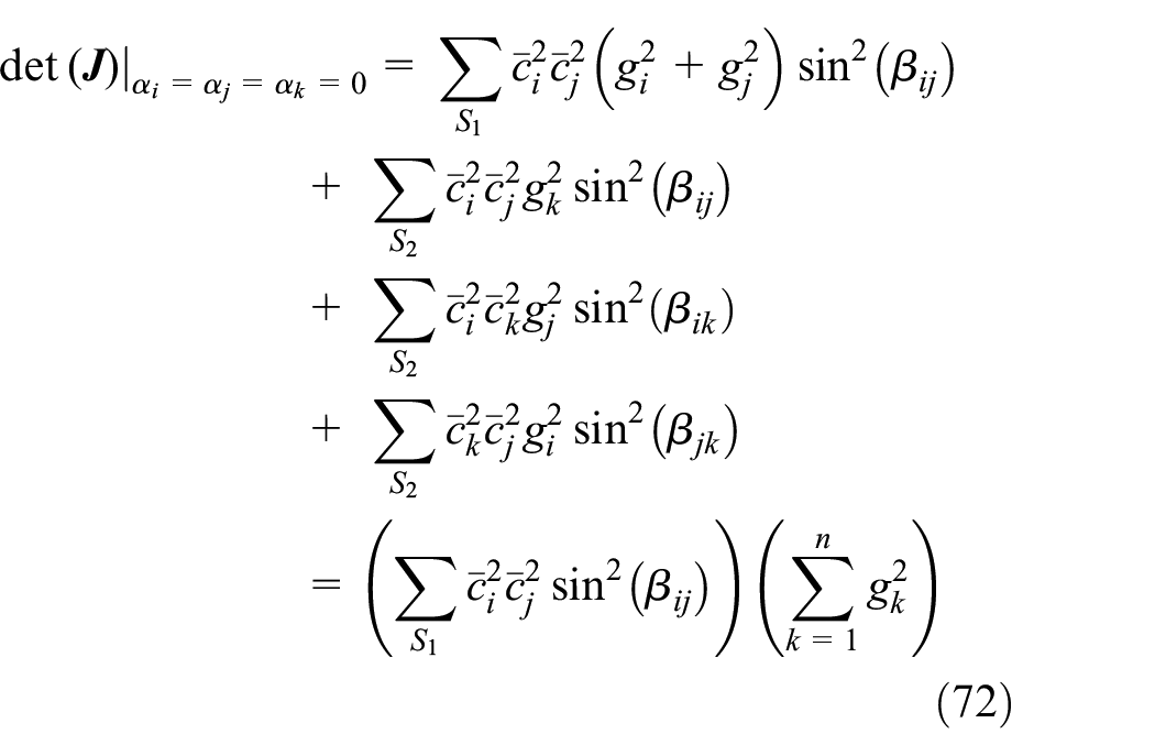
Recall the FIM in equation (21). Since $\mathit{J}$ is a $3\times 3$ symmetric matrix, represented by the product of $F{F}^{\top }$ , using the Cauchy–Binet formula, ⁴³ the determinant of $\mathit{J}$ can be calculated as

$$\det (\mathit{J})=\sum _{S_1}{\mathrm{\Lambda }}_1+\sum _{S_2}{\mathrm{\Lambda }}_2$$

(29)

where

$${\mathrm{\Lambda }}_1={|{\mathit{a}}_i,{\mathit{a}}_j,{\mathit{b}}_i|}^2+{|{\mathit{a}}_i,{\mathit{a}}_j,{\mathit{b}}_j|}^2+{|{\mathit{a}}_{\mathit{i}},{\mathit{b}}_i,{\mathit{b}}_j|}^2+{|{\mathit{a}}_j,{\mathit{b}}_i,{\mathit{b}}_j|}^2$$

(30)

$$\begin{array}{c}\multicolumn{1}{c}{{\mathrm{\Lambda }}_2={|{\mathit{a}}_i,{\mathit{a}}_j,{\mathit{a}}_k|}^2+{|{\mathit{b}}_i,{\mathit{b}}_j,{\mathit{b}}_k|}^2+{|{\mathit{a}}_i,{\mathit{a}}_j,{\mathit{b}}_k|}^2+{|{\mathit{a}}_k,{\mathit{b}}_i,{\mathit{b}}_j|}^2}\\ \multicolumn{1}{c}{+{|{\mathit{a}}_i,{\mathit{a}}_k,{\mathit{b}}_j|}^2+{|{\mathit{a}}_j,{\mathit{a}}_k,{\mathit{b}}_i|}^2+{|{\mathit{a}}_j,{\mathit{b}}_i,{\mathit{b}}_k|}^2+{|{\mathit{a}}_i,{\mathit{b}}_j,{\mathit{b}}_k|}^2}\end{array}$$

(31)

and

$$S_1=\{(i,j)|1\le i<j\le n\}$$

(32)

$$S_2=\{(i,j,k)|1\le i<j<k\le n\}$$

(33)

It is readily observed that the number of $S_1$ is $\left(\begin{array}{c}n\hfill \\ \multicolumn{1}{c}{2}\end{array}\right)$ , while the number of $S_2$ is $\left(\begin{array}{c}n\hfill \\ \multicolumn{1}{c}{3}\end{array}\right)$ . For $n=2$ , it follows immediately that the second term of $\sum _{S_2}{\mathrm{\Lambda }}_2$ in equation (29) does not exist.

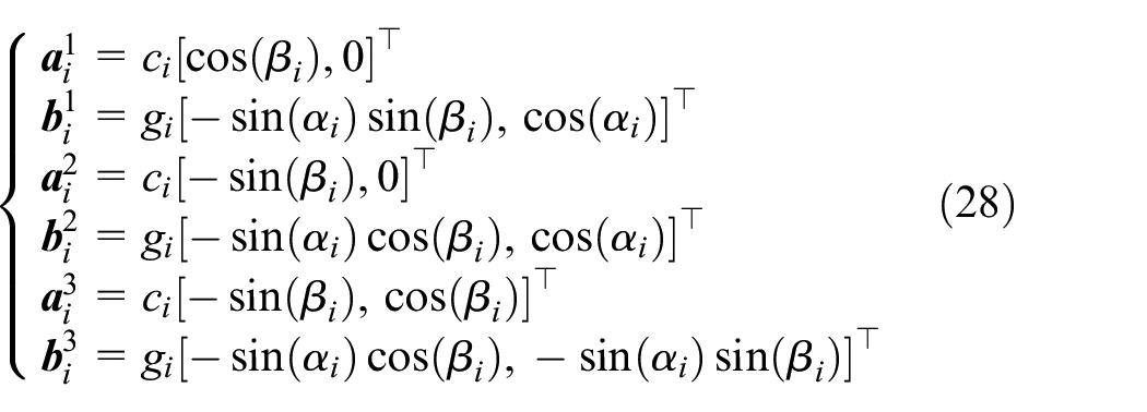
Recall the definitions of ${\mathit{a}}_i$ and ${\mathit{b}}_i$ in equation (19). The vectors of ${\mathit{a}}_j$ and ${\mathit{a}}_k$ in equations (30) and (31) are just generated by replacing the indices i with j and k from ${\mathbf{a}}_i$ , respectively. Similarly, the vectors of ${\mathit{b}}_j$ and ${\mathit{b}}_k$ can also be determined from the vector of ${\mathit{b}}_i$ . After some calculation, ${\mathrm{\Lambda }}_1$ can be represented as

$${\mathrm{\Lambda }}_1={\mathrm{\Delta }}_1^{d_1}(i,j)+{\mathrm{\Delta }}_1^{d_1}(j,i)+{\mathrm{\Delta }}_2^{d_1}(i,j)+{\mathrm{\Delta }}_2^{d_1}(j,i)$$

(34)

where

$$\begin{array}{c}\multicolumn{1}{c}{{\mathrm{\Delta }}_1^{d_1}(i,j)\stackrel{\mathrm{\Delta }}{=}{c}_i^2{g}_i^2{g}_j^2{[\sin \left({\alpha }_i\right)\cos \left({\alpha }_j\right)-\cos \left({\alpha }_i\right)\sin \left({\alpha }_j\right)\cos \left({\beta }_{\mathrm{ij}}\right)]}^2}\end{array}$$

(35)

$${\mathrm{\Delta }}_2^{d_1}(i,j)\stackrel{\mathrm{\Delta }}{=}{c}_i^2{c}_j^2{g}_j^2{\cos }^2\left({\alpha }_j\right){\sin }^2\left({\beta }_{\mathrm{ij}}\right)$$

(36)

with ${\beta }_{\mathrm{ij}}={\beta }_i-{\beta }_j$ . ${\mathrm{\Delta }}_1^{d_1}(j,i)$ , and ${\mathrm{\Delta }}_2^{d_1}(j,i)$ are generated from the definitions of ${\mathrm{\Delta }}_1^{d_1}(i,j)$ and ${\mathrm{\Delta }}_2^{d_1}(i,j)$ by exchanging the indices i and j, respectively, and vice versa, denoted as

$$\begin{array}{c}{\mathrm{\Delta }}_1^{d_1}(i,j)\stackrel{\stackrel{i\to j}{j\to i}}{\iff }{\mathrm{\Delta }}_1^{d_1}(j,i)\hfill \\ \multicolumn{1}{c}{{\mathrm{\Delta }}_2^{d_1}(i,j)\stackrel{\stackrel{i\to j}{j\to i}}{\iff }{\mathrm{\Delta }}_2^{d_1}(j,i)}\end{array}$$

(37)

In a similar fashion, ${\mathrm{\Lambda }}_2$ is calculated as follows

$$\begin{array}{c}\multicolumn{1}{c}{{\mathrm{\Lambda }}_2={\mathrm{\Delta }}_1^{d_2}(i,j,k)+{\mathrm{\Delta }}_1^{d_2}(i,k,j)+{\mathrm{\Delta }}_1^{d_2}(k,j,i)+{\mathrm{\Delta }}_2^{d_2}(i,j,k)}\\ \multicolumn{1}{c}{+{\mathrm{\Delta }}_2^{d_2}(j,i,k)+{\mathrm{\Delta }}_2^{d_2}(k,j,i)}\\ \multicolumn{1}{c}{+{[{\mathrm{\Delta }}_3^{d_2}(i,j,k)-{\mathrm{\Delta }}_3^{d_2}(i,k,j)-{\mathrm{\Delta }}_3^{d_2}(k,j,i)]}^2}\end{array}$$

(38)

where

$${\mathrm{\Delta }}_1^{d_2}(i,j,k)\stackrel{\mathrm{\Delta }}{=}{c}_i^2{c}_j^2{g}_k^2{\cos }^2\left({\alpha }_k\right){\sin }^2\left({\beta }_{\mathrm{ij}}\right)$$

(39)

$${\mathrm{\Delta }}_2^{d_2}(i,j,k)\stackrel{\mathrm{\Delta }}{=}{c}_i^2{g}_j^2{g}_k^2{\left[\begin{array}{c}\sin \left({\alpha }_j\right)\cos \left({\alpha }_k\right)\cos \left({\beta }_{\mathrm{ij}}\right)\hfill \\ \multicolumn{1}{c}{-\cos \left({\alpha }_j\right)\sin \left({\alpha }_k\right)\cos \left({\beta }_{\mathrm{ik}}\right)}\end{array}\right]}^2$$

(40)

$${\mathrm{\Delta }}_3^{d_2}(i,j,k)\stackrel{\mathrm{\Delta }}{=}{g}_i{g}_j{g}_k\sin ({\alpha }_i)\sin ({\alpha }_j)\cos ({\alpha }_k)\sin ({\beta }_{\mathrm{ij}})$$

(41)

with ${\beta }_{\mathrm{ij}}={\beta }_i-{\beta }_j$ and ${\beta }_{\mathrm{ik}}={\beta }_i-{\beta }_k$ . The corresponding transformations among the terms of ${\mathrm{\Lambda }}_2$ are given by

$$\begin{array}{c}{\mathrm{\Delta }}_1^{d_2}(k,j,i)\stackrel{\stackrel{i\to k}{k\to i}}{\iff }{\mathrm{\Delta }}_1^{d_2}(i,j,k)\stackrel{\stackrel{j\to k}{k\to j}}{\iff }{\mathrm{\Delta }}_1^{d_2}(i,k,j)\hfill \\ \multicolumn{1}{c}{{\mathrm{\Delta }}_2^{d_2}(k,j,i)\stackrel{\stackrel{i\to k}{k\to i}}{\iff }{\mathrm{\Delta }}_2^{d_2}(i,j,k)\stackrel{\stackrel{i\to j}{j\to i}}{\iff }{\mathrm{\Delta }}_2^{d_2}(j,i,k)}\\ \multicolumn{1}{c}{{\mathrm{\Delta }}_3^{d_2}(k,j,i)\stackrel{\stackrel{i\to k}{k\to i}}{\iff }{\mathrm{\Delta }}_3^{d_2}(i,j,k)\stackrel{\stackrel{j\to k}{k\to j}}{\iff }{\mathrm{\Delta }}_3^{d_2}(i,k,j)}\end{array}$$

(42)

Calculation of the cofactors of $f_{\mathrm{mm}}$

Following the similar manner of determining the determinant of $\mathit{J}$ , the determinants of ${\mathit{J}}_{\mathrm{mm}},m\in \{1,2,3\}$ can also be determined by using the Cauchy–Binet formula. ⁴³ Thus, the cofactors of $f_{\mathrm{mm}},m\in \{1,2,3\}$ in equation (26) can be calculated as follows

$$f_{\mathrm{mm}}=\det \left({\mathit{J}}_{\mathrm{mm}}\right)={\mathrm{\Omega }}_1^m+{\mathrm{\Omega }}_2^m$$

(43)

where

$${\mathrm{\Omega }}_1^m=\sum _{i=1}^n{|{\mathit{a}}_i^m,{\mathit{b}}_i^m|}^2$$

(44)

$${\mathrm{\Omega }}_2^m=\sum _{S_1}({|{\mathit{a}}_i^m,{\mathit{a}}_j^m|}^2+{|{\mathit{b}}_i^m,{\mathit{b}}_j^m|}^2+{|{\mathit{a}}_i^m,{\mathit{b}}_j^m|}^2+{|{\mathit{a}}_j^m,{\mathit{b}}_i^m|}^2)$$

(45)

Noting that the set of $S_1$ is defined in equation (32), the vectors of ${\mathit{a}}_i^m$ and ${\mathit{b}}_i^m$ are defined in equation (28), $m\in \{1,2,3\}$ . ${\mathit{a}}_j^m$ and ${\mathit{b}}_j^m$ can be generated just by using j instead of i from the definitions of the vectors ${\mathit{a}}_i^m$ and ${\mathit{b}}_i^m$ , respectively.

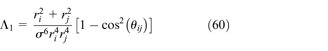
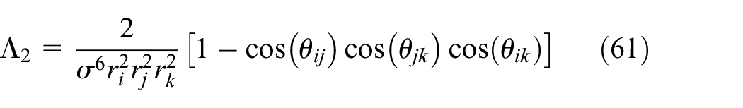
Using equation (43) to calculate each cofactor of $f_{\mathrm{mm}}$ , then adding all of them, after some algebra, leads to

$$\sum _{m=1}^3{f}_{\mathrm{mm}}=\sum _{i=1}^n{c}_i^2{g}_i^2+\sum _{S_1}{\mathrm{\Lambda }}_3$$

(46)

where

$${\mathrm{\Lambda }}_3={\mathrm{\Delta }}_1^{n_1}(i,j)+{\mathrm{\Delta }}_1^{n_1}(j,i)+{\mathrm{\Delta }}_2^{n_1}(i,j)+{\mathrm{\Delta }}_2^{n_1}(j,i)+{\mathrm{\Delta }}_3^{n_1}(i,j)$$

(47)

and

$${\mathrm{\Delta }}_1^{n_1}(i,j)\stackrel{\mathrm{\Delta }}{=}{c}_i^2{g}_j^2[{\cos }^2\left({\alpha }_j\right)+{\sin }^2\left({\alpha }_j\right){\cos }^2\left({\beta }_{\mathrm{ij}}\right)]$$

(48)

$$\begin{array}{c}\multicolumn{1}{c}{{\mathrm{\Delta }}_2^{n_1}(i,j)\stackrel{\mathrm{\Delta }}{=}{g}_i^2{g}_j^2}\\ \multicolumn{1}{c}{[{\cos }^2\left({\alpha }_i\right){\sin }^2\left({\alpha }_j\right)-\frac{1}{4}\cos \left({\beta }_{\mathrm{ij}}\right)\sin \left(2{\alpha }_i\right)\sin \left(2{\alpha }_j\right)]}\end{array}$$

(49)

$${\mathrm{\Delta }}_3^{n_1}(i,j)\stackrel{\mathrm{\Delta }}{=}[c_i^2{c}_j^2+g_i^2{g}_j^2{\sin }^2\left({\alpha }_i\right){\sin }^2\left({\alpha }_j\right)]{\sin }^2\left({\beta }_{\mathrm{ij}}\right)$$

(50)

with the transformations given by

$$\begin{array}{c}{\mathrm{\Delta }}_1^{n_1}(i,j)\stackrel{\stackrel{i\to j}{j\to i}}{\iff }{\mathrm{\Delta }}_1^{n_1}(j,i)\hfill \\ \multicolumn{1}{c}{{\mathrm{\Delta }}_2^{n_1}(i,j)\stackrel{\stackrel{i\to j}{j\to i}}{\iff }{\mathrm{\Delta }}_2^{n_1}(j,i)}\end{array}$$

(51)

Evaluation of the GDOP

Recall the definition of GDOP in equation (7), which requires that the FIM is invertible, that is, $\det (\mathit{J})\ne 0$ . Now, we first give the necessary and sufficient condition of $\det (\mathit{J})=0$ , then utilize the equivalence principle of a proposition and its contrapositive to obtain the corresponding condition of the invertibility of the FIM.

Theorem 1

• For $n=2$ AOA sensors, $\det (\mathit{J})=0$ if and only if the condition (i) holds; for $n\ge 3$ AOA sensors, $\det (\mathit{J})=0$ if and only if the condition (ii) holds.

• i.  $({\beta }_i,{\beta }_j,{\alpha }_i,{\alpha }_j)\in \left(\bigcup _{p=1}^2{\mathcal{A}}_p\right),\forall (i,j)\in S_1$ .

• ii. $({\beta }_i,{\beta }_j,{\beta }_k,{\alpha }_i,{\alpha }_j,{\alpha }_k)\in \left(\bigcup _{q=1}^4{\mathcal{B}}_q\right),\forall (i,j,k)\in S_2$ .

where

$$\{\begin{array}{c}{\mathcal{A}}_1=\{{\beta }_i={\beta }_j,{\alpha }_i={\alpha }_j\}\hfill \\ \multicolumn{1}{c}{{\mathcal{A}}_2=\{{\beta }_{\mathrm{ij}}=\pm \pi ,{\alpha }_i=-{\alpha }_j\}}\\ \multicolumn{1}{c}{{\mathcal{B}}_1=\{{\beta }_i={\beta }_j={\beta }_k,{\alpha }_i={\alpha }_j={\alpha }_k\}}\\ \multicolumn{1}{c}{{\mathcal{B}}_2=\{{\beta }_i={\beta }_j,{\beta }_{\mathrm{ik}}={\beta }_{\mathrm{jk}}=\pm \pi ,{\alpha }_i={\alpha }_j=-{\alpha }_k\}}\\ \multicolumn{1}{c}{{\mathcal{B}}_3=\{{\beta }_i={\beta }_k,{\beta }_{\mathrm{ij}}={\beta }_{\mathrm{jk}}=\pm \pi ,{\alpha }_i={\alpha }_k=-{\alpha }_j\}}\\ \multicolumn{1}{c}{{\mathcal{B}}_4=\{{\beta }_j={\beta }_k,{\beta }_{\mathrm{ij}}={\beta }_{\mathrm{ik}}=\pm \pi ,{\alpha }_j={\alpha }_k=-{\alpha }_i\}}\end{array}$$

(52)

and ${\alpha }_i\in (-\pi /2,\pi /2),{\beta }_i\in (-\pi ,\pi ],\forall i\in \{1,2,\dots ,n\}$ .

Proof

We will prove it by two steps.

• (a) Sufficiency: For $n=2$ sensors, the term $\sum _{S_2}{\mathrm{\Lambda }}_2$ in equation (29) does not exist, $\det (\mathit{J})=\sum _{S_1}{\mathrm{\Lambda }}_1$ . For all $(i,j)\in S_1$ , if $({\beta }_i,{\beta }_j,{\alpha }_i,{\alpha }_j)\in {\mathcal{A}}_1$ , then ${\beta }_{\mathrm{ij}}=0,{\alpha }_i={\alpha }_j$ , resulting in $\sin ({\beta }_{\mathrm{ij}})=0,\cos ({\beta }_{\mathrm{ij}})=1$ ; submitting them into equation (34), it follows immediately that ${\mathrm{\Lambda }}_1=0$ . In a similar fashion, if $({\beta }_i,{\beta }_j,{\alpha }_i,{\alpha }_j)\in {\mathcal{A}}_2$ , the same result of ${\mathrm{\Lambda }}_1=0$ can be achieved. Thus, $\forall (i,j)\in S_1$ , $({\beta }_i,{\beta }_j,{\alpha }_i,{\alpha }_j)\in (\bigcup _{p=1}^2{\mathcal{A}}_p)$ , we have ${\mathrm{\Lambda }}_1=0$ , then $\det (\mathit{J})=\sum _{S_1}{\mathrm{\Lambda }}_1=0$ .

For $n\ge 3$ sensors, $\det (\mathit{J})=\sum _{S_1}{\mathrm{\Lambda }}_1+\sum _{S_2}{\mathrm{\Lambda }}_2$ . For all $(i,j,k)\in S_2$ , if $({\beta }_i,{\beta }_j,{\beta }_k,{\alpha }_i,{\alpha }_j,{\alpha }_k)\in {\mathcal{B}}_1$ , then ${\beta }_{\mathrm{ij}}={\beta }_{\mathrm{ik}}={\beta }_{\mathrm{jk}}=0,{\alpha }_i={\alpha }_j={\alpha }_k$ , and we have $\sin ({\beta }_{\mathrm{ij}})=$ $\sin ({\beta }_{ik})=\sin ({\beta }_{jk})=0,\cos ({\beta }_{ij})=\cos ({\beta }_{ik})=\cos ({\beta }_{jk})=1$ . Note that exchanging the indices of i and j, or i and k, or j and k, the above two continued equalities still hold. Submitting $\sin ({\beta }_{ij})=\sin ({\beta }_{ji})=0,\cos ({\beta }_{ij})=\cos ({\beta }_{ji})=1$ into equation (34) and $\sin ({\beta }_{ij})=\sin ({\beta }_{ik})=\sin ({\beta }_{kj})=0,$ $\cos ({\beta }_{\mathrm{ij}})=\cos ({\beta }_{\mathrm{ji}})=\cos ({\beta }_{\mathrm{kj}})=1,\cos ({\beta }_{\mathrm{ik}})=\cos ({\beta }_{\mathrm{jk}})=\cos ({\beta }_{\mathrm{ki}})=1$ into equation (38), respectively, leads to ${\mathrm{\Lambda }}_1=0$ and ${\mathrm{\Lambda }}_2=0$ . Similarly, for the remaining cases, one can obtain the same results of ${\mathrm{\Lambda }}_1=0$ and ${\mathrm{\Lambda }}_2=0$ for each case. Thus, $\forall (i,j,k)\in S_2$ , $({\beta }_i,{\beta }_j,{\beta }_k,{\alpha }_i,{\alpha }_j,{\alpha }_k)\in (\bigcup _{q=1}^4{\mathcal{B}}_q)$ , it follows immediately that ${\mathrm{\Lambda }}_1=0$ and ${\mathrm{\Lambda }}_2=0$ , which leads to $\sum _{S_1}{\mathrm{\Lambda }}_1=0$ and $\sum _{S_2}{\mathrm{\Lambda }}_2=0$ , and then $\det (\mathit{J})=0$ . Therefore, the sufficient conditions (i) and (ii) are both true.

• (b) Necessity: for $n=2$ sensors, $det(\mathit{J})=0$ is equivalent to the case of $\forall (i,j)\in S_1,{\mathrm{\Lambda }}_1=0$ . According to equation (34), ${\mathrm{\Lambda }}_1=0$ leads to ${\mathrm{\Delta }}_1^{d_1}(i,j)={\mathrm{\Delta }}_1^{d_1}(j,i)={\mathrm{\Delta }}_2^{d_1}(i,j)={\mathrm{\Delta }}_2^{d_1}(j,i)=0$ . From ${\mathrm{\Delta }}_2^{d_1}(i,j)=0$ , we have $\sin ({\beta }_{\mathrm{ij}})=0$ , which yields ${\beta }_{\mathrm{ij}}=0$ or ${\beta }_{\mathrm{ij}}=\pm \pi$ for ${\beta }_{\mathrm{ij}}\in (-2\pi ,2\pi )$ . Inserting ${\beta }_{\mathrm{ij}}=0$ and ${\beta }_{\mathrm{ij}}=\pm \pi$ into ${\mathrm{\Delta }}_1^{d_1}(i,j)=0$ by equation (35), resulting in ${\alpha }_{\mathrm{ij}}=0$ and ${\alpha }_i=-{\alpha }_j$ , respectively. Note that for ${\beta }_{\mathrm{ij}}=0$ and ${\beta }_{\mathrm{ij}}=\pm \pi$ , the solutions of ${\alpha }_{\mathrm{ij}}=\pm \pi$ and ${\alpha }_i+{\alpha }_j=\pm \pi$ are ruled out for ${\alpha }_i,{\alpha }_j\in (-\pi /2,\pi /2)$ , respectively. Similarly, by ${\mathrm{\Delta }}_2^{d_1}(j,i)={\mathrm{\Delta }}_1^{d_1}(j,i)=0$ , yields ${\beta }_{\mathrm{ji}}=0,{\alpha }_{\mathrm{ij}}=0$ and ${\beta }_{\mathrm{ji}}=\pm \pi ,{\alpha }_i=-{\alpha }_j$ , which is equivalent to the case of ${\mathrm{\Delta }}_1^{d_1}(i,j)={\mathrm{\Delta }}_2^{d_1}(i,j)=0$ . Denoting the sets of solutions to ${\mathrm{\Lambda }}_1=0$ as ${\mathcal{A}}_1=\{{\beta }_i={\beta }_j,{\alpha }_i={\alpha }_j\}$ and ${\mathcal{A}}_2=\{{\beta }_{\mathrm{ij}}=\pm \pi ,{\alpha }_i=-{\alpha }_j\}$ , and then the condition (i) is obtained.

For $n\ge 3$ sensors, $\det (\mathit{J})=0$ leads to $\forall (i,j)\in S_1,{\mathrm{\Lambda }}_1=0$ and $\forall (i,j,k)\in S_2,{\mathrm{\Lambda }}_2=0$ by equation (29). For the case of $\forall (i,j)\in S_1,{\mathrm{\Lambda }}_1=0$ , following the procedure of $n=2$ sensors, the same results can be achieved as those of the condition (i). For all $(i,j,k)\in S_2,{\mathrm{\Lambda }}_2=0$ , yielding each term of ${\mathrm{\Lambda }}_2$ in equation (38) equals to zero, that is

$${\mathrm{\Delta }}_1^{d_2}(i,j,k)={\mathrm{\Delta }}_1^{d_2}(i,k,j)={\mathrm{\Delta }}_1^{d_2}(k,j,i)=0$$

(53)

$${\mathrm{\Delta }}_2^{d_2}(i,j,k)={\mathrm{\Delta }}_2^{d_2}(j,i,k)={\mathrm{\Delta }}_2^{d_2}(k,j,i)=0$$

(54)

$${\mathrm{\Delta }}_3^{d_2}(i,j,k)-{\mathrm{\Delta }}_3^{d_2}(i,k,j)-{\mathrm{\Delta }}_3^{d_2}(k,j,i)=0$$

(55)

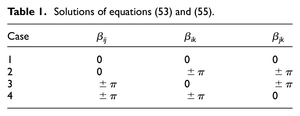
Using equations (39) and (42), noting that $\sin ({\beta }_{\mathrm{jk}})=0$ is equivalent to $\sin ({\beta }_{\mathrm{kj}})=0$ , the solutions to equations (53) and (55) are readily obtained from $\sin ({\beta }_{\mathrm{ij}})=\sin ({\beta }_{\mathrm{ik}})=\sin ({\beta }_{\mathrm{jk}})=0$ , that is, ${\beta }_{\mathrm{ij}}\in \{0,\pm \pi \},{\beta }_{\mathrm{ik}}\in \{0,\pm \pi \}$ and ${\beta }_{\mathrm{jk}}\in \{0,\pm \pi \}$ . Note that any one term of ${\beta }_{\mathrm{ij}},{\beta }_{\mathrm{ik}},$ and ${\beta }_{\mathrm{jk}}$ can be determined from the other two terms. Then all solutions of equations (53) and (55) are determined and listed in Table 1.

Table 1.

Solutions of equations (53) and (55).

Case	${\beta }_{\mathrm{ij}}$	${\beta }_{\mathrm{ik}}$	${\beta }_{\mathrm{jk}}$
1	0	0	0
2	0	$\pm \pi$	$\pm \pi$
3	$\pm \pi$	0	$\pm \pi$
4	$\pm \pi$	$\pm \pi$	0

For each case in Table 1, submitting the values of ${\beta }_{\mathrm{ij}},{\beta }_{\mathrm{ik}},$ and ${\beta }_{\mathrm{jk}}$ into equation (54), leads to ${\alpha }_i={\alpha }_j={\alpha }_k$ , ${\alpha }_i={\alpha }_j=-{\alpha }_k$ , ${\alpha }_i={\alpha }_k=-{\alpha }_j,$ and ${\alpha }_j={\alpha }_k=-{\alpha }_i$ , respectively. Thus, for all $(i,j,k)\in S_2$ , the solutions to ${\mathrm{\Lambda }}_2=0$ consist of four different sets, given by

• i. ${\mathcal{B}}_1=\{{\beta }_i={\beta }_j={\beta }_k,{\alpha }_i={\alpha }_j={\alpha }_k\}$ ;

• ii. ${ℬ}_2=\left\{{\beta }_i={\beta }_j,{\beta }_{ik}={\beta }_{jk}=\pm \pi ,{\alpha }_i={\alpha }_j=-{\alpha }_k\right\}$ ;

• iii. ${ℬ}_3=\left\{{\beta }_i={\beta }_k,{\beta }_{ij}={\beta }_{jk}=\pm \pi ,{\alpha }_i={\alpha }_k=-{\alpha }_j\right\}$ ;

• iv. ${ℬ}_4=\left\{{\beta }_j={\beta }_k,{\beta }_{ij}={\beta }_{ik}=\pm \pi ,{\alpha }_j={\alpha }_k=-{\alpha }_i\right\}$ .

Recall the solutions of ${\mathrm{\Lambda }}_1=0$ , that is, ${\mathcal{A}}_1$ and ${\mathcal{A}}_2$ , which are inherently included in the solutions of ${\mathrm{\Lambda }}_2=0$ . Thus, the condition (ii) in Theorem 1 can be achieved. In combination with the analyses of (a) and (b), the proof of Theorem 1 is completed.

As previously stated, for simplicity, we use the notations of ${\beta }_{\mathrm{ij}}={\beta }_i-{\beta }_j$ and ${\alpha }_{\mathrm{ij}}={\alpha }_i-{\alpha }_j$ in equation (52), and so on. From the condition (i), for $n=2$ sensors, it follows immediately that two sensors are collinear with the target of ${\mathit{p}}_t$ . For $({\beta }_i,{\beta }_j,{\alpha }_i,{\alpha }_j)\in {\mathcal{A}}_1$ , two sensors are located at the same side with respect to the target on the line, while for $({\beta }_i,{\beta }_j,{\alpha }_i,{\alpha }_j)\in {\mathcal{A}}_2$ , two sensors are separately located at the two sides of the line against the target. Similarly, investigating the condition (ii) for $n\ge 3$ sensors, it is also shown that all sensors are collinear with the target ${\mathit{p}}_t$ . For each $(i,j,k)\in S_2$ , there are two cases of sensor–target geometries: one is that three sensors are all located at the same side of the line against the target if $({\beta }_i,{\beta }_j,{\beta }_k,{\alpha }_i,{\alpha }_j,{\alpha }_k)\in {\mathcal{B}}_1$ , and the second is that two sensors are located at the same side and the remainder is located at the opposite side against the target when $({\beta }_i,{\beta }_j,{\beta }_k,{\alpha }_i,{\alpha }_j,{\alpha }_k)\in ({\mathcal{B}}_2\cup {\mathcal{B}}_3\cup {\mathcal{B}}_4)$ . Hence, we have the following corollary.

Corollary 1

• The conditions of (i) and (ii) in Theorem 1 are equivalent to the single condition that all AOA sensors of ${\mathit{s}}_i$ are collinear with the target ${\mathit{p}}_t$ with ${\alpha }_i\in (-\pi /2,\pi /2),{\beta }_i\in (-\pi ,\pi ],\forall i\in \{1,2,\dots ,n\}$ .

Therefore, the alternative form of Theorem 1 can be represented as follows.

Theorem 2

• For ${\alpha }_i\in (-\pi /2,\pi /2),{\beta }_i\in (-\pi ,\pi ],\forall i\in \{1,2,\dots ,n\}$ , $\det (\mathit{J})=0$ if and only if all AOA sensors of ${\mathit{s}}_i$ are collinear with the target ${\mathit{p}}_t$ .

Proof

Using Theorem 1 and Corollary 1, the result can be readily obtained and then this completes the proof.

Since the condition in Theorem 2 is necessary and sufficient, using the equivalence principle of propositions, the contrapositive and inverse of Theorem 2 are both true, which can be represented by the following corollary.

Corollary 2

For ${\alpha }_i\in (-\pi /2,\pi /2),{\beta }_i\in (-\pi ,\pi ],\forall i\in \{1,2,\cdots ,n\}$ , the FIM of $\mathit{J}$ is invertible, that is, $\det (\mathit{J})\ne 0$ , if and only if there exists at least a pair of sensors $(i,j)\in S_1$ that are non-collinear with the target ${\mathit{p}}_t$ .

If the sensors i and j are non-collinear with the target ${\mathit{p}}_t$ , then $({\beta }_i,{\beta }_j,{\alpha }_i,{\alpha }_j)\notin ({\mathcal{A}}_1\cup {\mathcal{A}}_2)$ and $|\cos ({\theta }_{\mathrm{ij}})|\ne 1$ , note that ${\theta }_{\mathrm{ij}}$ is the angle of LOS between sensors i and j; thus, we have another form of Corollary 2, given as follows.

Corollary 3

For ${\alpha }_i\in (-\pi /2,\pi /2),{\beta }_i\in (-\pi ,\pi ],\forall i\in \{1,2,\dots ,n\}$ , the FIM of $\mathit{J}$ is invertible, that is, $\det (\mathit{J})\ne 0$ , if and only if there exists at least a pair of sensors $(i,j)\in S_1$ such that $({\beta }_i,{\beta }_j,{\alpha }_i,{\alpha }_j)\notin ({\mathcal{A}}_1\cup {\mathcal{A}}_2)$ or $|\cos ({\theta }_{\mathrm{ij}})|\ne 1$ .

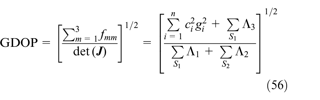
According to Corollary 2, if $\exists (i,j)\in S_1$ , the corresponding sensors i and j are non-collinear with the target ${\mathit{p}}_t$ , and then $\det (\mathit{J})\ne 0$ , and the GDOP exists for $n\ge 2$ sensors in 3D AOA target localization. In this case, putting equations (29) and (46) into equation (25), then the complete closed form of the GDOP for 3D AOA sensors target localization can be obtained, given by

$$\mathrm{GDOP}={\left[\frac{\sum _{m=1}^3{f}_{\mathrm{mm}}}{det(\mathit{J})}\right]}^{1/2}={\left[\frac{\sum _{i=1}^n{c}_i^2{g}_i^2+\sum _{S_1}{\mathrm{\Lambda }}_3}{\sum _{S_1}{\mathrm{\Lambda }}_1+\sum _{S_2}{\mathrm{\Lambda }}_2}\right]}^{1/2}$$

(56)

As noted before, for $n=2$ AOA sensors, the term of $\sum _{S_2}{\mathrm{\Lambda }}_2$ in equation (56) does not exist. Note that any additional assumptions are not made on the number of sensors, the observation ranges, and noise variances for the derivation of GDOP. The derived GDOP in equation (56) is a more general closed form with explicit expression.

For $n\ge 2$ AOA sensors, the sets of data for calculating the GDOP are collected as below

$$S_{\beta }={\left\{{\beta }_i\right\}}_{i=1}^n,S_{\alpha }={\left\{{\alpha }_i\right\}}_{i=1}^n,S_c={\left\{c_i\right\}}_{i=1}^n,S_g={\left\{g_i\right\}}_{i=1}^n$$

(57)

A concise procedure of evaluating the GDOP in equation (54) is listed in Algorithm 1.

Algorithm 1. Procedure of evaluating the GDOP for 3D AOA target localization.
Input: the sets of data $S_{\beta },S_{\alpha },S_c,$ and $S_g$ Output: the value of the GDOP 1: For each $i\in \{1,2,\dots ,n\}$ , calculate $c_i^2{g}_i^2$ and then add all the terms of $c_i^2{g}_i^2$ by $\sum _{i=1}^n{c}_i^2{g}_i^2$
2: For each $(i,j)\in S_1$ , calculate ${\mathrm{\Lambda }}_3$ and ${\mathrm{\Lambda }}_1$ by equations (47) and (34), respectively, then add all the terms of ${\mathrm{\Lambda }}_3$ and ${\mathrm{\Lambda }}_1$ by $\sum _{S_1}{\mathrm{\Lambda }}_3$ and $\sum _{S_1}{\mathrm{\Lambda }}_1$ , respectively
3: For each $(i,j,k)\in S_2$ , calculate ${\mathrm{\Lambda }}_2$ by equation (38) and then add all the terms of ${\mathrm{\Lambda }}_2$ by $\sum _{S_2}{\mathrm{\Lambda }}_2$
4: Calculate the GDOP using equation (56)
5: return $\mathrm{GDOP}$

GDOP: geometric dilution of precision; AOA: angle-of-arrival.

Special case studies

Now, in this section, we will show that, for some special cases, the formulas of GDOP for AOA target localization in some existing works can be directly deduced from the proposed formula of equation (56).

Special case: $\sigma ={\sigma }_{{\alpha }_i}={\sigma }_{{\beta }_i}\cos ({\alpha }_i)$

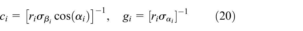
For the case in Zhong et al., ¹² the assumption is made on the observation noise variances of ${\sigma }_{{\beta }_i}^2$ and ${\sigma }_{{\alpha }_i}^2$ for the derivation of GDOP, that is, $\sigma ={\sigma }_{{\alpha }_i}={\sigma }_{{\beta }_i}\cos ({\alpha }_i),\forall i\in \{1,2,\dots ,n\}$ . It is readily observed that the singular points of ${\alpha }_i=\pm \pi /2$ are ruled out for $\sigma >0$ . In this case, the terms of $c_i$ and $g_i$ in equation (20) become

$$c_i=g_i=[r_i\sigma {]}^{-1}$$

(58)

Submitting equation (58) into equation (46), which yields

$$\begin{array}{c}\multicolumn{1}{c}{\sum _{i=1}^n{c}_i^2{g}_i^2+\sum _{S_1}{\mathrm{\Lambda }}_3=\sum _{i=1}^n\frac{1}{{\sigma }^4{r}_i^4}+\sum _{S_1}\frac{1}{{\sigma }^4{r}_i^2{r}_j^2}}\\ \multicolumn{1}{c}{[3-{\cos }^2\left({\theta }_{\mathrm{ij}}\right)]}\end{array}$$

(59)

where ${\theta }_{\mathrm{ij}}$ is the angle of LOS between sensor i and sensor j. Using equation (58), the term ${\mathrm{\Lambda }}_1$ in equation (34) is given by

$${\mathrm{\Lambda }}_1=\frac{r_i^2+r_j^2}{{\sigma }^6{r}_i^4{r}_j^4}[1-{\cos }^2\left({\theta }_{\mathrm{ij}}\right)]$$

(60)

Correspondingly, ${\mathrm{\Lambda }}_2$ in equation (38) can be determined as

$${\mathrm{\Lambda }}_2=\frac{2}{{\sigma }^6{r}_i^2{r}_j^2{r}_k^2}[1-\cos \left({\theta }_{\mathrm{ij}}\right)\cos \left({\theta }_{\mathrm{jk}}\right)\cos \left({\theta }_{\mathrm{ik}}\right)]$$

(61)

where the angles of ${\theta }_{\mathrm{ij}},{\theta }_{\mathrm{jk}},$ and ${\theta }_{\mathrm{ik}}$ can be determined by the unit vectors of LOS of sensors $i,j,\mathrm{and}k$ , given by

$$\begin{array}{c}{\mathit{u}}_i={[\cos \left({\alpha }_i\right)\cos \left({\beta }_i\right),\cos \left({\alpha }_i\right)\sin \left({\beta }_i\right),\sin \left({\alpha }_i\right)]}^{\top }\hfill \\ \multicolumn{1}{c}{{\mathit{u}}_j={[\cos \left({\alpha }_j\right)\cos \left({\beta }_j\right),\cos \left({\alpha }_j\right)\mathrm{in}\left({\beta }_j\right),\sin \left({\alpha }_j\right)]}^{\top }}\\ \multicolumn{1}{c}{{\mathit{u}}_k={[\cos \left({\alpha }_k\right)\cos \left({\beta }_k\right),\cos \left({\alpha }_k\right)\sin \left({\beta }_k\right),\sin \left({\alpha }_k\right)]}^{\top }}\end{array}$$

(62)

Using the inner products among the vectors of ${\mathit{u}}_i,{\mathit{u}}_j,$ and ${\mathit{u}}_k$ , one obtains

$$\begin{array}{c}\cos \left({\theta }_{\mathrm{ij}}\right)=〈{\mathit{u}}_i,{\mathit{u}}_j〉\hfill \\ \multicolumn{1}{c}{\cos \left({\theta }_{\mathrm{jk}}\right)=〈{\mathit{u}}_j,{\mathit{u}}_k〉}\\ \multicolumn{1}{c}{\cos \left({\theta }_{\mathrm{ik}}\right)=〈{\mathit{u}}_i,{\mathit{u}}_k〉}\end{array}$$

(63)

Therefore, the same results as those of Zhong et al. ¹² with the assumption of $\sigma ={\sigma }_{{\alpha }_i}={\sigma }_{{\beta }_i}\cos ({\alpha }_i)$ can be achieved.

Special case: 2D AOA target localization

Following the similar fashion of deriving the FIM for 3D case, the FIM for 2D case is given by

$$\overline{\mathit{J}}=\sum _{i=1}^n{\overline{a}}_i{\overline{a}}_i^{\mathrm{T}}=\overline{\mathit{F}}{\overline{\mathit{F}}}^{\top }$$

(64)

where

$$\overline{\mathit{F}}=[{\overline{a}}_1,\dots ,{\overline{a}}_n]$$

(65)

and

$${\overline{a}}_i={\overline{c}}_i{[-\sin \left({\beta }_i\right),\cos \left({\beta }_i\right)]}^{\mathrm{T}},{\overline{c}}_i={\left[r_i{\sigma }_{{\beta }_i}\right]}^{-1}$$

(66)

Using the Cauchy–Binet formula again, ⁴³ the determinant of $\overline{\mathit{J}}$ is calculated as

$$\det (\overline{\mathit{J}})=\sum _{S_1}|{\overline{\mathit{a}}}_i,{\overline{\mathit{a}}}_j{|}^2=\sum _{S_1}{\overline{c}}_i^2{\overline{c}}_j^2{\sin }^2\left({\beta }_{\mathrm{ij}}\right)$$

(67)

Noting that $\overline{\mathit{J}}\in {\mathbb{R}}^{2\times 2}$ , if $\overline{\mathit{J}}$ is invertible, then we have

$$\mathrm{tr}({\overline{\mathit{J}}}^{-1})=\frac{\mathrm{tr}(\overline{\mathit{J}})}{\det (\overline{\mathit{J}})}=\frac{1}{\det (\overline{\mathit{J}})}\sum _{i=1}^n{\overline{c}}_i^2$$

(68)

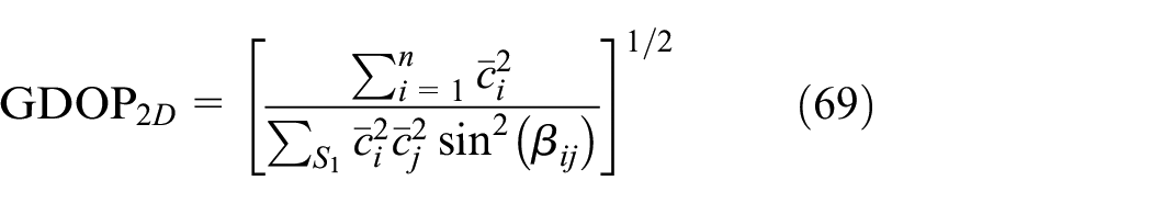
Thus, the GDOP for 2D AOA target localization is determined by

$$\mathrm{GDO}{\mathrm{P}}_{2D}={\left[\frac{\sum _{i=1}^n{\overline{c}}_i^2}{\sum _{S_1}{\overline{c}}_i^2{\overline{c}}_j^2{\sin }^2\left({\beta }_{\mathrm{ij}}\right)}\right]}^{1/2}$$

(69)

Actually, the GDOP for 2D AOA target localization can be directly determined from the formula of equation (56) just by removing the term of $f_{33}$ and setting ${\alpha }_i=0,\forall i\in \{1,2,\dots ,n\}$ , then the GDOP for 2D case becomes

$$\mathrm{GDO}{\mathrm{P}}_{2\mathrm{D}}={{\left[\frac{\sum _{m=1}^2{f}_{\mathrm{mm}}}{det(\mathbf{J})}\right]}^{1/2}|}_{{\alpha }_i={\alpha }_j={\alpha }_k=0}$$

(70)

where

$$\begin{array}{c}\sum _{m=1}^2{f}_{\mathrm{mm}}{|}_{{\alpha }_i={\alpha }_j=0}=\sum _{i=1}^n{\overline{c}}_i^2{g}_i^2+\sum _{S_1}({\overline{c}}_i^2{g}_j^2+{\overline{c}}_j^2{g}_i^2)\hfill \\ =\sum _{i=1}^n\sum _{j=1}^n{\overline{c}}_i^2{g}_j^2\hfill \\ =\left(\sum _{i=1}^n{\overline{c}}_i^2\right)\left(\sum _{j=1}^n{g}_j^2\right)\hfill \end{array}$$

(71)

and

$$\begin{array}{c}det(\mathit{J}){|}_{{\alpha }_i={\alpha }_j={\alpha }_k=0}=\sum _{S_1}{\overline{c}}_i^2{\overline{c}}_j^2(g_i^2+g_j^2){\sin }^2\left({\beta }_{\mathrm{ij}}\right)\hfill \\ +\sum _{S_2}{\overline{c}}_i^2{\overline{c}}_j^2{g}_k^2{\sin }^2\left({\beta }_{\mathrm{ij}}\right)\hfill \\ +\sum _{S_2}{\overline{c}}_i^2{\overline{c}}_k^2{g}_j^2{\sin }^2\left({\beta }_{\mathrm{ik}}\right)\hfill \\ +\sum _{S_2}{\overline{c}}_k^2{\overline{c}}_j^2{g}_i^2{\sin }^2\left({\beta }_{\mathrm{jk}}\right)\hfill \\ =\left(\sum _{S_1}{\overline{c}}_i^2{\overline{c}}_j^2{\sin }^2\left({\beta }_{\mathrm{ij}}\right)\right)\left(\sum _{k=1}^n{g}_k^2\right)\hfill \end{array}$$

(72)

Submitting equations (71) and (72) into equation (70), it follows immediately that the same result as that of equation (69) can be obtained.

Similarly, following Corollary 2 and considering equations (67) and (69), noting that there are no singularities in 2D AOA target localization for the target and sensors with distinct locations, the necessary and sufficient condition for the invertibility of the FIM (or the existence of GDOP) for 2D AOA target localization can be readily obtained, given by the following corollaries.

Corollary 4

For 2D AOA target localization, the FIM of $\overline{\mathit{J}}$ is invertible (or the GDOP exists), if and only if there exists at least a pair of sensors $(i,j)\in S_1$ that are non-collinear with the target.

Corollary 5

For 2D AOA target localization, the FIM of $\overline{\mathit{J}}$ is invertible (or the GDOP exists), if and only if there exists at least a pair of sensors $(i,j)\in S_1$ such that ${\beta }_{\mathrm{ij}}\notin \{0,\pm \pi \}$ .

Illustrative examples

In this section, we propose some examples to illustrate the evaluation of GDOP for 3D AOA target localization with different sensor–target geometries. In addition, in practice, circular error probable (CEP) is also often used as a measure of a localization/navigation system (e.g. GPS/GNSS) precision. Here, we also use CEP to show the target localization accuracy for the following simulations.

In the considered AOA target localization scenario, the RMS of target location estimation error can attain the CRLB with any unbiased estimator. Therefore, the CEP can be approximated by the following formula ⁴⁴

$$\mathrm{CEP}\approx 0.83\times \mathrm{RMS}\approx 0.83\times \mathrm{GDOP}$$

In the following simulations, the GDOP and the approximate CEP are all calculated and provided.

It is worthwhile to point out first that, our derived results can handle the general case for sensors with different z coordinates, since the results in our work are strictly derived for the general scenario in AOA target localization, where sensors can be deployed in 3D space with different altitudes. For intuitive representation of our results, in Examples 2 and 3, all the sensors are set to be with identical z coordinates.

Example 1

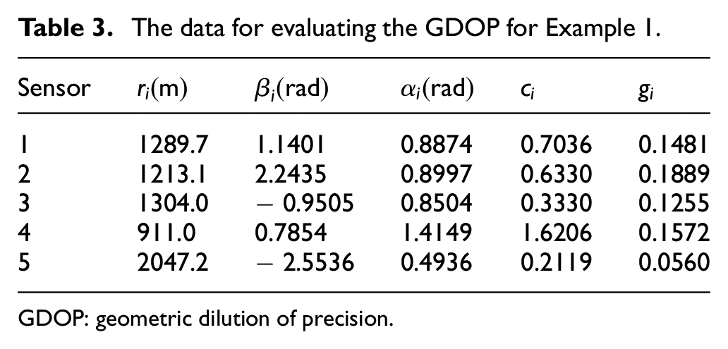
Consider $n=5$ AOA sensors used for 3D target localization. The location of the target is set to be ${\mathit{p}}_t=[500\mathrm{m},800\mathrm{m},1000\mathrm{m}{]}^{\top }$ , and the other simulation parameters with respect to the sensors are listed in Table 2. Note that the sensor noise variances of ${\sigma }_{{\beta }_i}^2$ and ${\sigma }_{{\alpha }_i}^2$ can be different or identical from each other, and no restrictive assumption on the noise variances is made for the evaluation of GDOP. The sets of $S_{\beta }=\{{\beta }_i{\}}_{i=1}^5,S_{\alpha }=\{{\alpha }_i{\}}_{i=1}^5,S_c=\{c_i{\}}_{i=1}^5$ and $S_g=\{g_i{\}}_{i=1}^5$ including $\{r_i{\}}_{i=1}^5$ for the evaluation of GDOP are collected and listed in Table 3. The sensor–target geometry is shown in Figure 2, where the solid black squares indicate the AOA sensors, and the solid red triangles denote the target. From Table 3 and Figure 2, it is readily observed that sensors 1 and 2 are non-collinear with the target of ${\mathit{p}}_t$ , by Corollary 2, the FIM for this case is invertible and the GDOP exists. Using the procedure of Algorithm 1, the GDOP is readily calculated as 5.7674 m (and the approximate CEP is 4.7869 m).

Table 2.

The simulation parameters for Example 1.

Sensor	$x_i(\mathrm{m})$	$y_i(\mathrm{m})$	$z_i(\mathrm{m})$	${\sigma }_{{\beta }_i}(\mathrm{deg})$	${\sigma }_{{\alpha }_i}(\mathrm{deg})$
1	160	60	0	0.1	0.3
2	970	210	50	0.1	0.3
3	0	1500	20	0.2	0.3
4	400	700	100	0.3	0.4
5	2000	1800	30	0.1	0.5

Table 3.

The data for evaluating the GDOP for Example 1.

Sensor	$r_i(\mathrm{m})$	${\beta }_i(\mathrm{rad})$	${\alpha }_i(\mathrm{rad})$	$c_i$	$g_i$
1	1289.7	1.1401	0.8874	0.7036	0.1481
2	1213.1	2.2435	0.8997	0.6330	0.1889
3	1304.0	−0.9505	0.8504	0.3330	0.1255
4	911.0	0.7854	1.4149	1.6206	0.1572
5	2047.2	−2.5536	0.4936	0.2119	0.0560

GDOP: geometric dilution of precision.

Figure 2.

The sensor–target geometry of Example 1 with $n=5$ AOA sensors.

Example 2

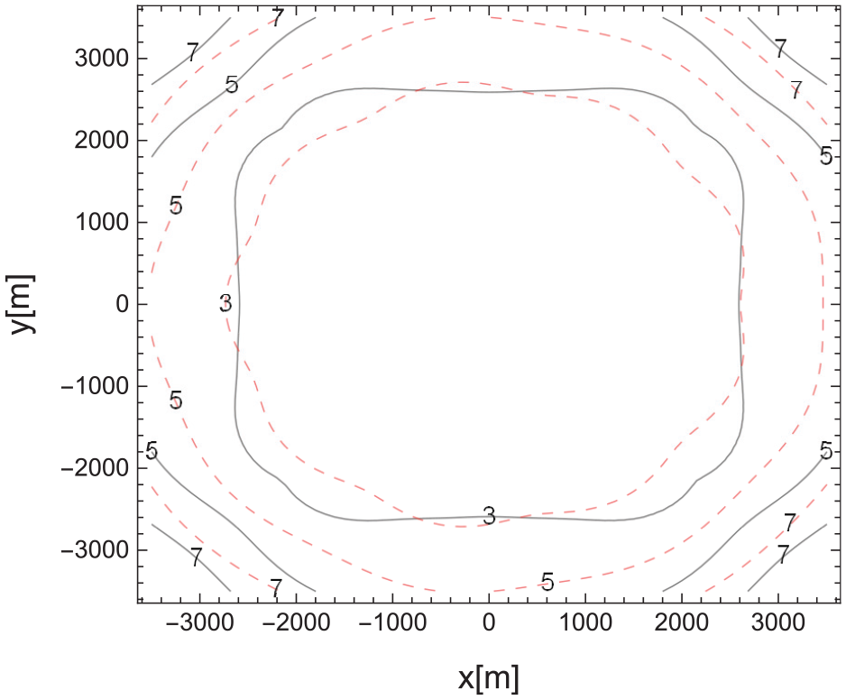
In this case, $n=7$ sensors are randomly distributed in the 3D Cartesian coordinate system of Oxyz, ranging from −2000 to 2000 m along the x-axis, −2000 to 2000 m along the y-axis and 0–500 m along the z-axis. The GDOP is evaluated on the region of $x_t\in [-3500\mathrm{m},3500\mathrm{m}],y_t\in [-3500\mathrm{m},3500\mathrm{m}]$ for targets with a constant $z_t=H_0=1000$ m height in the 3D space. The contour plot of GDOP is presented in Figure 3, and the contour map of CEP is depicted in Figure 4, where the solid white squares denote the AOA sensors. It can be readily observed that the values of GDOP are with obvious differences in different sensor–target geometries. The regions close to the center of the sensors are with a good localization accuracy of $\mathrm{GDOP}\le 5$ m, but the other regions with a little farther away from the center of the sensors are with relatively high values of GDOP, especially the lower left one in Figure 3, where the values of GDOP increase rapidly.

Table 4.

The simulation parameters for Example 2.

Sensor	$x_i(\mathrm{m})$	$y_i(\mathrm{m})$	$z_i(\mathrm{m})$	${\sigma }_{{\beta }_i}(\mathrm{deg})$	${\sigma }_{{\alpha }_i}(\mathrm{deg})$
1	−462	1931	409	0.2	0.3
2	332	921	130	0.1	0.3
3	−993	−624	297	0.2	0.1
4	−838	336	11	0.3	0.3
5	468	−1569	213	0.3	0.3
6	−939	1625	156	0.2	0.5
7	1298	1519	81	0.1	0.2

Figure 3.

The contours of GDOP for Example 2.

Figure 4.

The contours of CEP for Example 2.

Example 3

In this case, we consider two regular configurations for the deployment of $n=9$ AOA sensors. The first is that the $n=9$ AOA sensors are evenly spaced in a rectangular region from −2000 to 2000 m along the x-axis and −2000 to 2000 m along the y-axis, while the second is that the $n=9$ AOA sensors are deployed at the circumference by equiangular separations with a radius of 2000 m centered at the origin. All sensors in the above two regular configurations are with the same heights of $z_i=0$ m, and the standard deviations of ${\sigma }_{{\beta }_i}$ and ${\sigma }_{{\alpha }_i}$ are all set to be $0.1°,\forall i\in \{1,2,\cdots ,9\}$ . The region of the evaluation of GDOP for targets is the same as that of Example 2.

The contours of GDOP and CEP for the two regular configurations are depicted in Figures 5 and 6, and Figures 7 and 8, respectively. With the comparison of Figures 5 and 7, it is observed that the rectangular configuration of sensors in Figure 5 is comparable with or even better than the circular configuration in Figure 7, since it is clearly shown that in Figure 9, the region with the same level of GDOP in Figure 5 is generally larger than the one in Figure 7 when the values of GDOP contour levels are greater than 3 m. Indeed, the two proposed regular configurations of AOA sensors are all better than the one with random deployment of AOA sensors of Example 2. Moreover, in 2D AOA target localization, sensors deployed around the target by equiangular separations with identical observation ranges and noise variances are an optimal sensor–target geometry. ⁴⁵ However, noting that the contours of GDOP in Figure 7, the center (origin) of the AOA sensors with equiangular separations is not the point with the smallest GDOP value for 3D case.

Figure 5.

The contours of GDOP for rectangular configuration of Example 3.

Figure 6.

The contours of CEP for rectangular configuration of Example 3.

Figure 7.

The contours of GDOP for circular configuration of Example 3.

Figure 8.

The contours of CEP for circular configuration of Example 3.

Figure 9.

The contours of GDOP for rectangular and circular configurations of Example 3.

In practice, it is usually expected that the sensors are deployed with a good sensor–target geometry. Some performance measures concerning the accuracy of target localization including the determinant of the FIM and its inverse of the CRLB are adopted and optimized directly or indirectly to realize optimal sensor–target geometries. Based on different performance measures and methodologies, the optimal sensor configurations for 2D and/or 3D target localization using AOA and/or range-only sensors are, respectively, achieved by Xu and Doğançay ³³ and Zhao et al. ⁴⁶ These approaches can be extensively used to realize some optimal sensor–target geometries for single static target in 2D and/or 3D . For multiple targets localization, especially for the situation that multiple AOA passive sensors are required to be pre-deployed at a specific region where the targets may unexpectedly penetrate into such defense space, the aforementioned methods on the optimal sensor placement might not be competent for such case. As shown in Figures 5 and 7, the proposed analytical formula of GDOP in equation (56) can be used in advance to assess the sensor–target geometry for the surveillant region, then the results can be further used to determine preferred sensor–target geometries. For the results of Figures 5 and 7, one would prefer the rectangular configuration of Figure 5, where any target within the rectangular region from −2000 to 2000 m along the x-axis and −2000 to 2000 m along the y-axis, the values of GDOP are all less than 3 m. Indeed, the proposed analytical formula of GDOP can be used as a general objective function to be minimized for the optimal deployment of AOA sensors in 3D target localization.

Conclusion

In this article, we proposed a more general analytical formula of GDOP for 3D target localization using AOA sensors. Unlike the existing works in the literature, for the derivation of GDOP, the observation noise variances of AOA sensors are assumed to strictly satisfy a continued equality constraint, or the observation ranges and noise variances are assumed to be identical. In our method, no restrictive assumptions are made on the number of sensors, the observation ranges, and noise variances. The analytical formula of GDOP is obtained by using the Cauchy–Binet formula on the derived FIM. Moreover, a necessary and sufficient condition of the invertibility of the FIM is given, which can be used to judge the existence of GDOP. A concise procedure of evaluating the GDOP is also proposed, and then some examples are used to demonstrate the effectiveness of the presented approach.

As pointed out by Schmitt and Fichter, ⁴⁰ under the frame of spherical coordinates, the use of elevation and azimuth angles inevitably introduces singularities in 3D AOA target localization when ${\alpha }_i=\pm \pi /2$ . It is worthwhile to develop some new descriptions of the observation model of 3D AOA target localization for avoiding the aforementioned singularities. A unit vector observation model adopted in Zhao et al. ⁴⁶ may be suitable to overcome the problem of singularities. In future work, we will try to develop some new observation models including the unit vector model and attitude quaternion model for 3D AOA target localization. Then we will use these new observation models to investigate the performance measure as well as the optimal deployment for 3D AOA target localization.