
Abstract
The aim of this paper is to evaluate the performance of different filtering algorithms in the presence of non-Gaussian noise environment for tracking underwater targets, using Doppler frequency and bearing measurements. The tracking using Doppler frequency and bearing measurements is popularly known as Doppler-bearing tracking. Here the measurements, that is, bearings and Doppler frequency, are considered to be corrupted with two types of non-Gaussian noises namely shot noise and Gaussian mixture noise. The non-Gaussian noise sampled measurements are assumed to be obtained (a) randomly throughout the process and (b) repeatedly at some particular time samples. The efficiency of these filters with the increase in non-Gaussian noise samples is discussed in this paper. The performance of filters is compared with that of Cramer-Rao Lower Bound. Doppler-bearing extended Kalman filter and Doppler-bearing unscented Kalman filter are chosen for this work.
Keywords
Introduction
Target tracking is an important aspect of applicable electronic warfare and underwater surveillance. It is commonly performed using the measurements obtained from the sensors such as hull-mounted array. But these measurements are corrupted with noise. In practical scenarios, the noise is a mixture of non-Gaussian and Gaussian distributions. The tracking algorithms are developed to work under Gaussian as well as non-Gaussian noise (NGN). But these algorithms are not completely tested for their performance in NGN environment. The authors are inspired by the work done by Izanloo et al. 1 The NGN models for generating shot noise and Gaussian mixture noise are represented in this paper.
For marine applications, underwater target tracking is an important fundamental concept. 2 The objective behind tracking is to estimate the state of a moving target with the help of nonlinear measurements. The numerical approximation is mainly employed for several estimation methods in which the Monte Carlo method is very popular because of its flexibility in solution convergence. 3 In practical, all algorithms are sophisticated and mainly relied on approximations. In this research paper, the scenarios are considered in a two-dimensional plane. In underwater target tracking applications, observer continuously monitors for the signals that are generated due to the radiated noise of the target. Here the velocity of the target is pretended to be stationary. Target tracking is generally carried out using sonar in several naval applications. Measurements in the tonals that are extracted from the frequency spectrum (i.e. measured frequency) of the target are known as Doppler effect. In the frequency spectrum, the distinct frequency lines are considered to determine the target location.4–6 If both bearing and frequency measurements are attainable among any one of these distinct lines, then the target is said to be fully observable. The method where both bearing and frequency measurements (i.e. Doppler-bearing measurements) are processed and used to track the estimated path of the moving target is known as Doppler-bearing tracking (DBT).7–9
The aim of DBT is to determine the trajectory of the target based on a time series of Doppler and bearing measurements from a single observer. Estimates of target motion parameters (TMP; i.e. bearing, range, course, frequency and speed) are obtained more accurately by considering Doppler-bearing measurements.10–13 The passive tracking of a target using angle-only measurements using the line of sight (LOS) joining the target and observer is an important field of research in the application area. S-maneuver is performed on the LOS by the observer to obtain the observability of the target.
Kalman filter (KF) theory was evolved for linear Gaussian models which are discrete in time and is optimal filter for these models. KF fails for nonlinear application so extended Kalman filter (EKF) was implemented for such type of applications due to its sub-optimality.14,15 In the case of high nonlinearity, EKF becomes unstable, so in such cases unscented Kalman filter (UKF) was proposed by Julier and Uhlmann to overcome this problem. In many tracking applications, EKF gives erratic estimated results due to its unstable behavior. Therefore, UKF algorithm was implemented to overcome this problem.16–18 This UKF method captures the posterior covariance and mean very accurately for any second-order nonlinear system by propagating a set of selected sigma points recursively.
The relationship between the target position and Doppler-bearing measurements describes the significance of nonlinearity in the equations which is a challenging task in DBT. Therefore, EKF and UKF algorithms are modified accordingly to implement them for DBT application which are called Doppler-bearing extended Kalman filter (DBEKF) and Doppler-bearing unscented Kalman filter (DBUKF) algorithms. DBEKF is mainly based on the Taylor series approximation whereas DBUKF is based on unscented transformation (UT).19–22 In UT, sigma points, based on mean and covariance of the state, are selected deterministically. The selected sigma points are disseminated through a nonlinear function. These disseminated sigma points estimate the moments of the transformed variable from each sigma points. The nonlinear transformation causes higher order moments which are efficiently captured by UT. This makes UT advantageous over the Taylor series–based approximation.
To check the best convergence time of the solution for the algorithms, the implementation of two scenarios is discussed in the “Simulation results” section. Both DBEKF and DBUKF algorithms are implemented in MATLAB environment to evaluate their performance. The scenarios depicting the real-time situation are chosen for this research work, which is explained in section “Simulation results” of this paper. In the literature,10–16 the filter performances are evaluated under Gaussian noise environment only. For example, in the literature,23–28 it is simply stated that the performance of EKF and UKF is not satisfactory if the measurements and/or states are contaminated with NGN and therefore, it is suggested to use particle filter (PF). This is also evident from the derivations of the filters. In practice, filtering application is present to evaluate stochastic models disturbed with NGNs. With a large number of random samples, general probability distributions can be approximated properly using Monte Carlo sampling. 29
For non-Gaussian stochastic systems, EKF is recurrently shown to be abortive, where the noises can be shot noise or Gaussian mixture noise.16,23–25,30,31 In this research paper, the outcome of both shot and mixed-Gaussian noises for the given scenarios is analyzed by performing 100 Monte Carlo runs for both DBEKF and DBUKF algorithms. To enhance stability in state estimation under non-Gaussian environment, Monte Carlo simulation is performed for both nonlinear filters (DBEKF and DBUKF) to get the approximation of any probability distribution.
In the case of time-invariant statistical models, a commonly used lower boundary is the Cramér–Rao lower bound (CRLB). CRLB is calculated as the inverse of the Fisher information matrix. CRLB represents a basic lower boundary on estimate for the variance of an unbiased estimate. 32 Therefore, CRLB gives an adapted way to differentiate the performance of an unbiased estimator. It gives a best achievable performance of unbiased estimator, that is, lowest possible variance that can be achieved by an unbiased estimator. CRLB is a competent tool to determine the fulfillment of any algorithm for estimation. In DBT, DBUKF algorithm gives estimates that are close to the CRLB as compared to DBEKF algorithm which gives estimators far away from CRLB.26–28
In this paper, state estimation in the presence of NGN is discussed. Many filtering algorithms have been explained to cope with NGN. Importance of this work is to find the kinematics of the target with the help of available bearing and frequency measurements which are corrupted with NGNs. The performance evaluation of DBEKF and DBUKF algorithms in the presence of shot and Gaussian mixture noise is explained in this paper. Mathematical modeling for both DBEKF and DBUKF in the presence of Gaussian and NGNs is explained in this research paper. The sections of paper are organized as follows. Section “Mathematical modeling” gives a brief description about mathematical modeling of the state and measurement models, filtering algorithms and the concept behind CRLB applicable to the experiments investigated. Simulation and results are explained in section “Simulation results” and the conclusion is given in section “Conclusion.”
Mathematical modeling
State and measurement equations
It is assumed that the target moves with a constant speed and in a linear path. Two types of measurements are available from the set of measured data; they are frequency and bearing measurements. The equation of measured bearing is

where

where
Measured frequency is obtained from the observer due to Doppler shift as follows
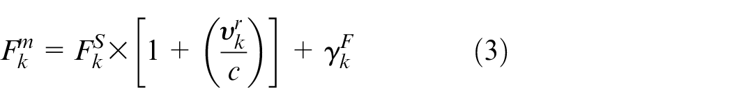
where

where


Equation (3) is rewritten in terms of measured frequency as

Therefore

Measurement vector

where
State vector of the target,
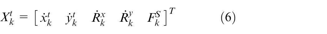
where
State vector of the observer,
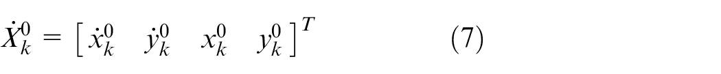
where
DBEKF algorithm
In bearings-only tracking (BOT) and other underwater applications, EKF is used with single bearing measurement. But in DBEKF, there are two measurements. Therefore, the calculation part of the algorithm is a little bit complicated and also needs changes in simulation of algorithm. Hence, it is named as DBEKF algorithm.
The state equation of the target is

where
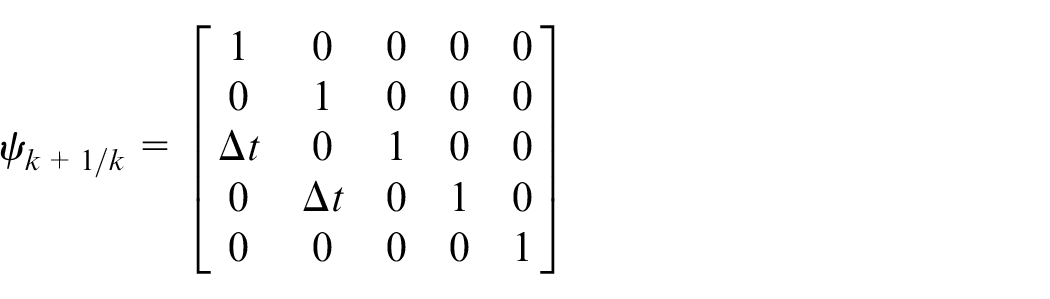
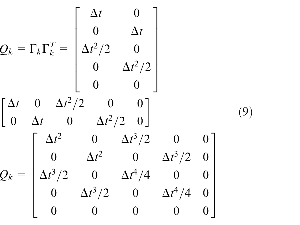
where
Here variance in plant noise is given as

where
Measurement equation is given as follows

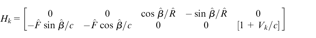
Measurement matrix is given as follows

where
Noise in the measurement equation is represented as

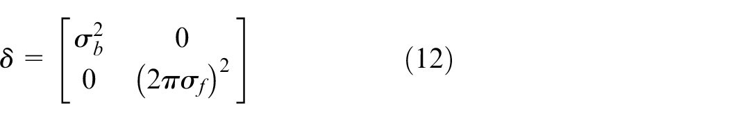
δ represents the measurement covariance matrix.
Time update of estimated covariance error is
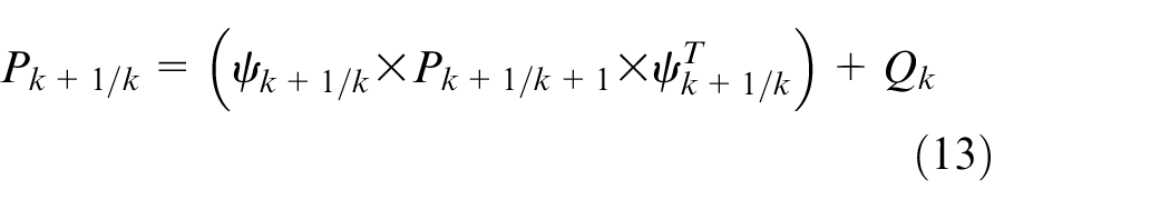
Time update of the state estimation is

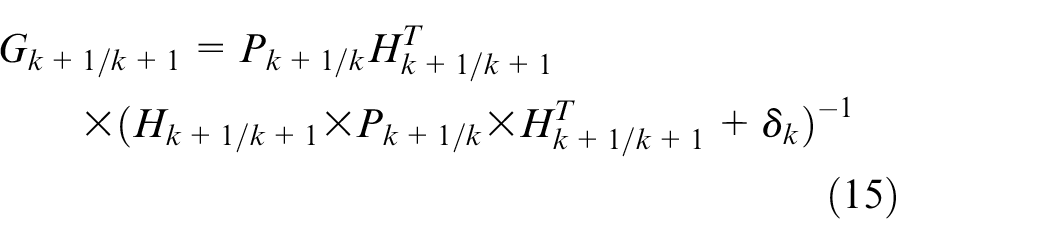
The Kalman gain is represented as
Updated state error covariance measurements are given as follows
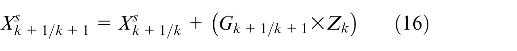
where
The flow diagram of DBEKF algorithm is described in Figure 1.
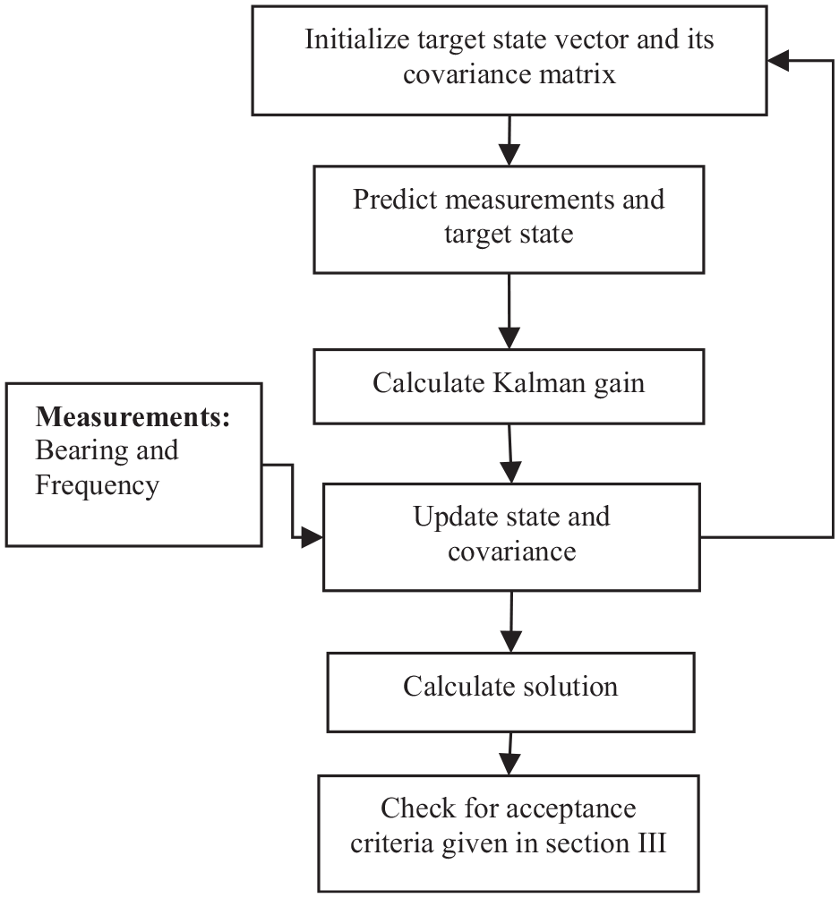
Flow diagram for DBEKF algorithm.
Unscented Transformation
The nonlinear transformation of a random variable is computed by an UT. Assume
where

By applying posterior sigma points, the mean and covariance weights are compared.
DBUKF algorithm
In BOT and other underwater applications, the UKF is used with single bearing measurement. But in DBUKF, there are two measurements. Therefore, the calculation part of the algorithm is a little bit complicated and also needs changes in simulation of algorithm. Hence, it is named as DBUKF algorithm.
The step-by-step algorithm for DBUKF is explained as follows:
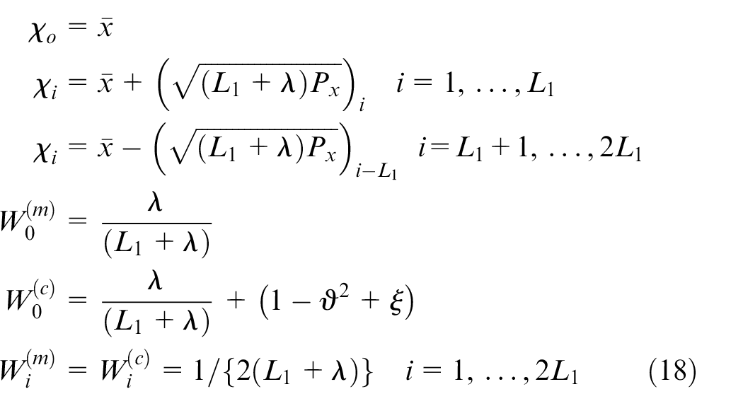
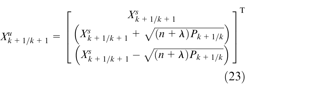
Taking n as the dimension of target state vector, the sigma points for
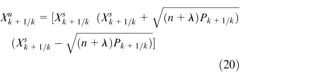
The transformation of sigma points is calculated from the process model (equation (8))
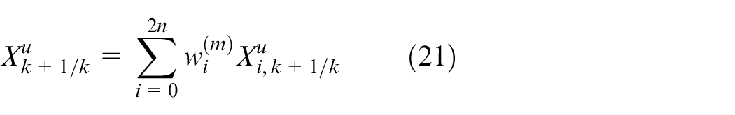
The predicted state estimate is given as
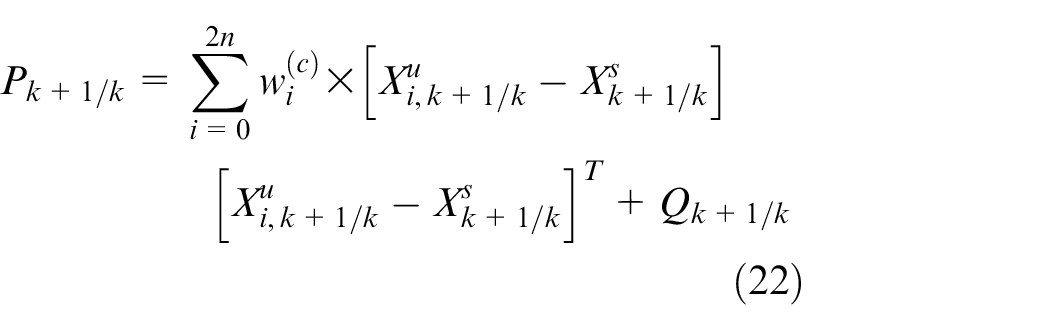
Predicted covariance is given as
The predicted mean for the given sigma points is updated as follows
From the measurement model (equation (22)), the transformation of each predicted point is calculated.
The measurement prediction
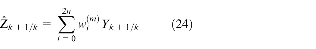
where

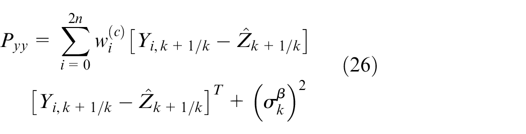
Innovation covariance is represented as
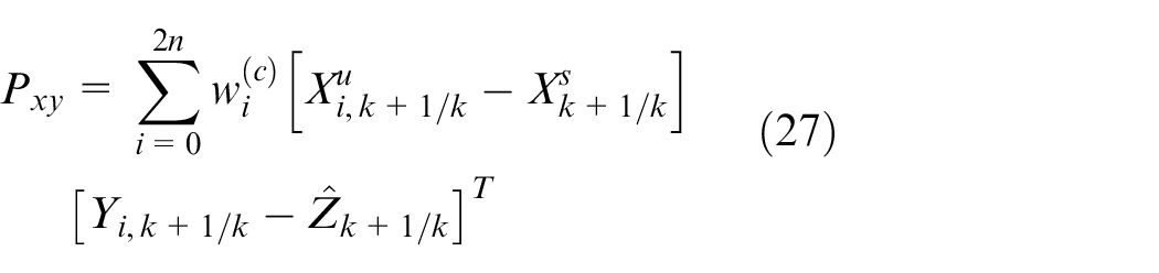
Cross-covariance is represented as
The gain is calculated as
The estimated state and error covariance are shown as follows
The flow of DBUKF algorithm is described in Figure 2.
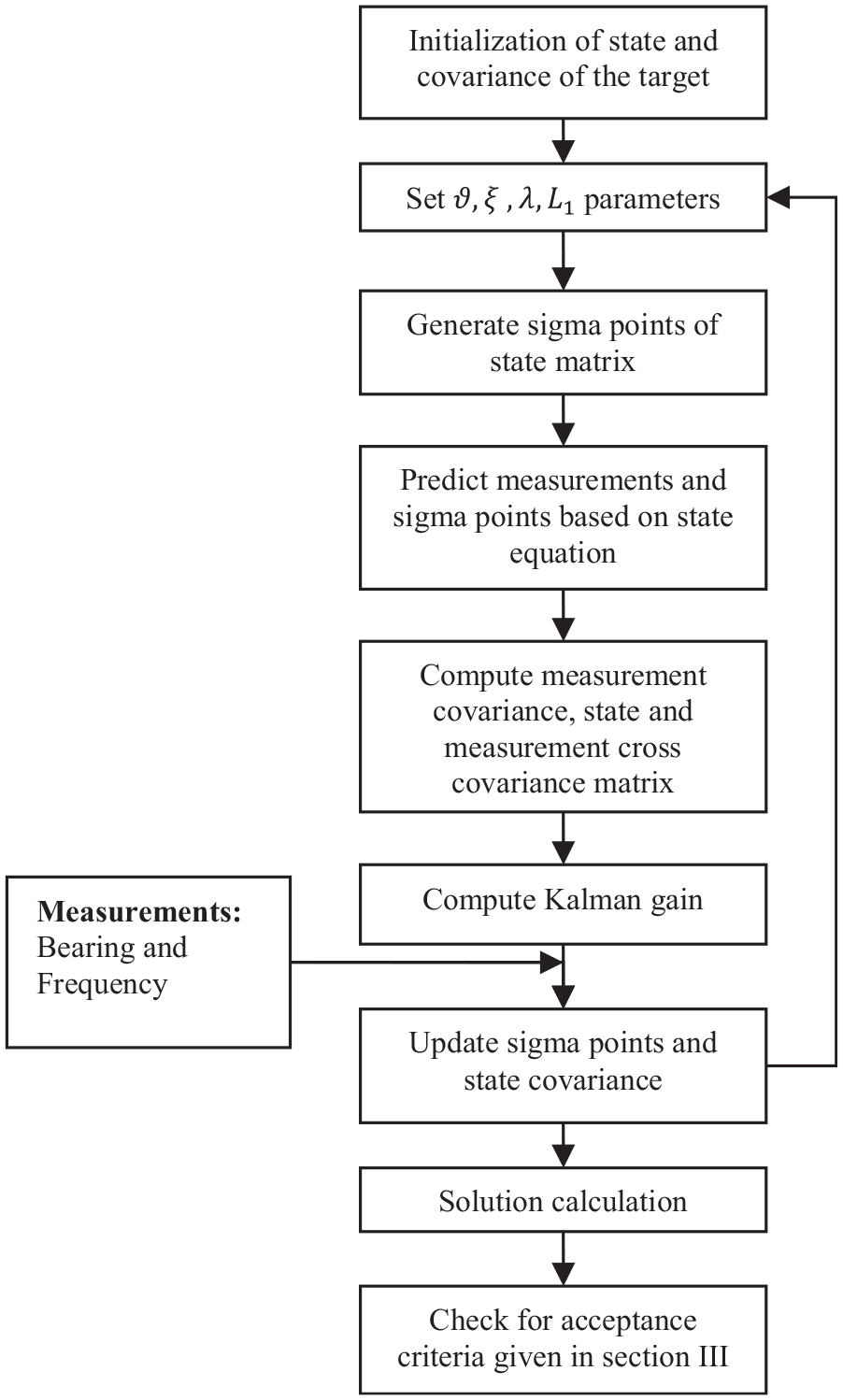
Flow diagram for DBUKF algorithm.
Cramer-Rao Lower Bound
For a nonlinear system which is discrete, the covariance of the estimated state is given as
where
The additive Gaussian noise is given in terms of


The Jacobian of the measurement function is given as
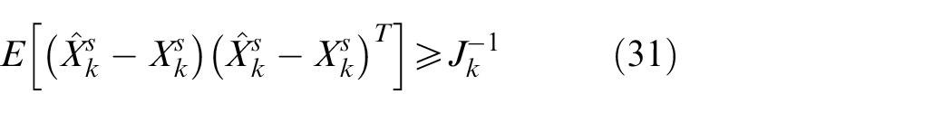
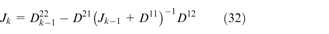
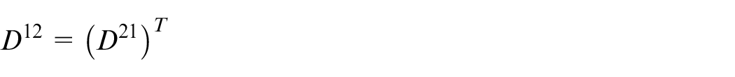
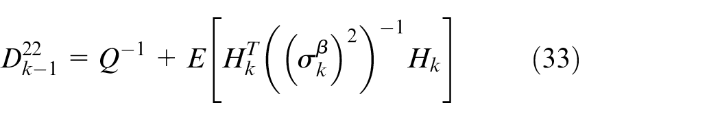
Now the CRLB of position error can be defined as

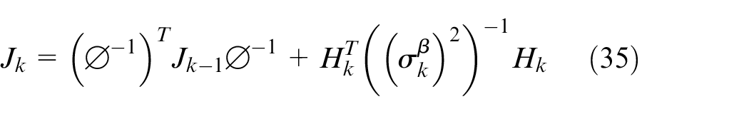
In the case of plant noise is considered as zero or not, then the information matrix is calculated recursively as
Non-Gaussian Noises
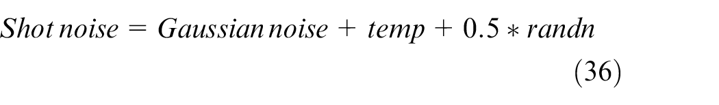
In this research work, the authors considered two types of NGNs which are shot and Gaussian mixture noises. Shot noise occurs due to statistical disturbances in the signal itself. In the case of shot noise, there will be a sudden increase or decrease in the noise amplitude. The same is carried out in MATLAB using “randn” function, in which some random high amplitude noise is added along with Gaussian noise as follows
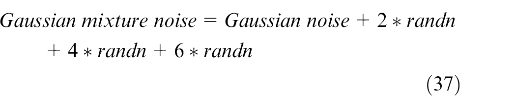
In Gaussian mixture noise, each noise sample has a mixture of different Gaussian variances. Therefore, Gaussian mixture noise is generated by adding Gaussian noises having different variances as follows
The histograms of the spread of the noise samples used for simulation for different noises are shown in Figures 3 and 4.
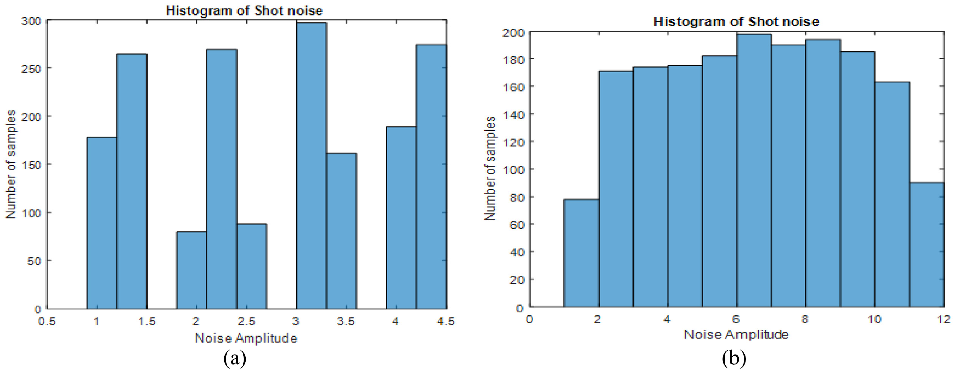
Histogram for shot noise used in this work: (a) bearing measurement and (b) frequency measurement.
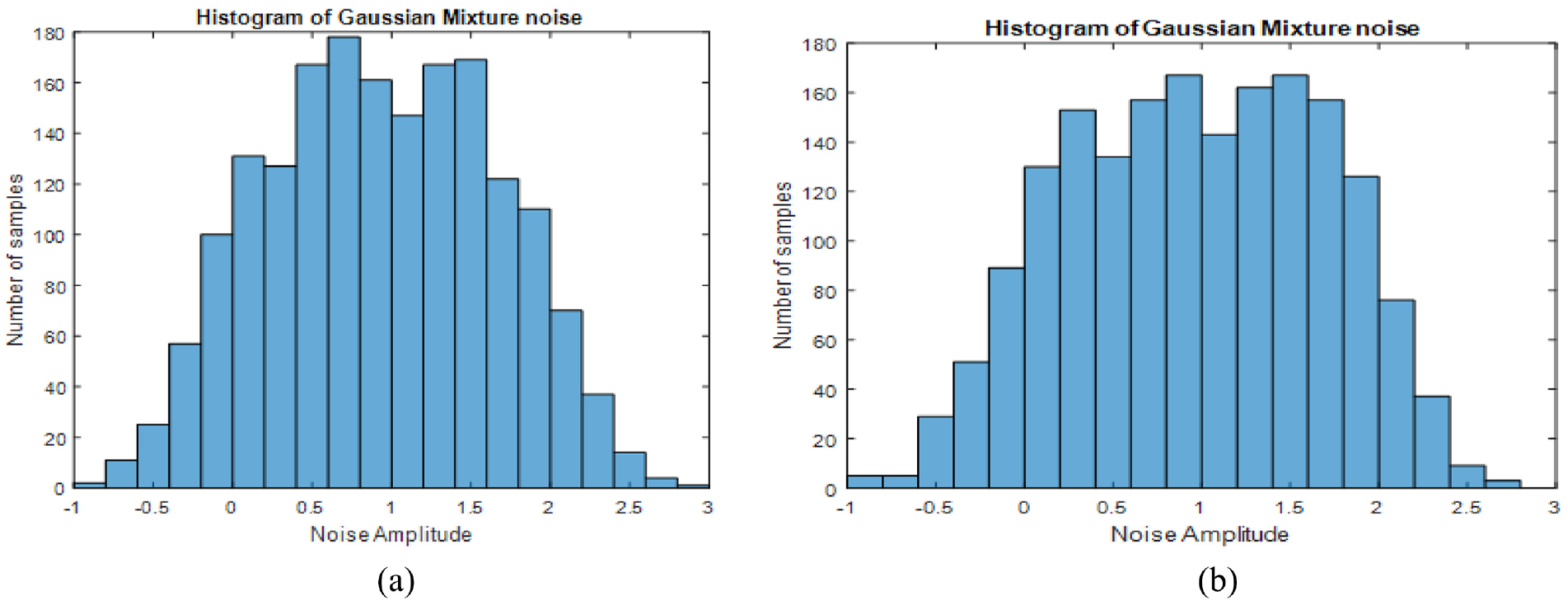
Histogram for Gaussian mixture noise used in this work: (a) bearing measurement and (b) frequency measurement.
Simulation results
In this research paper, the performance evaluation of both the algorithms is implemented in MATLAB PC environment. For every 1 s, the measurements are assumed to be available continuously. In this paper, the observer performs S-maneuver on the LOS with a turn rate of 0.5°/s. The observer is maneuvering in its course to obtain the observability of the target. Therefore, the observer initially has a course of 90° for 2 min and then turns 180° in order to attain the first leg and has a course of 270°. The observer is considered to take 4 min for complete maneuver of 180°. Observer has to perform S-maneuver on the initially observed LOS. Therefore, the initial bearing is chosen as 0° for simplicity in scenarios. By choosing 0° for initial bearing, error in bearing at initial stage is very high. The maximum change in bearing is from 0° to 359°, which makes a major change in bearing rate, making the error very high. Hence, the precision of the filter is also tested in the presence of maximum error in bearing measurement.
The frequency and bearing measurements are assumed to be corrupted with noises following white Gaussian distribution, having a standard deviation (SD) of 0.33 Hz and
Observer and target scenarios.
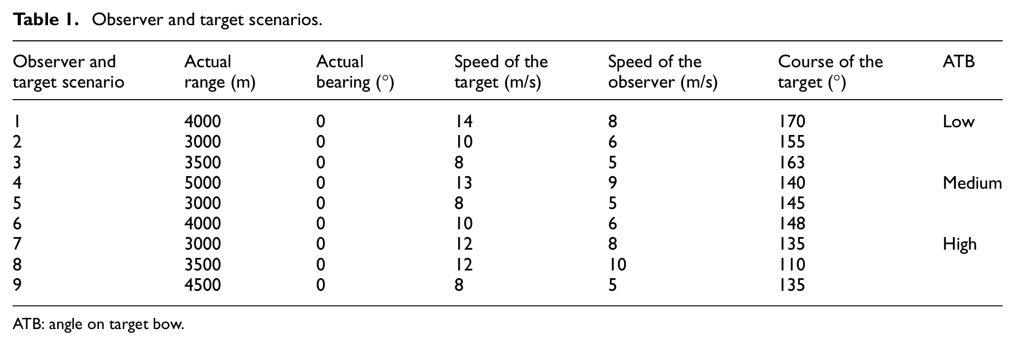
ATB: angle on target bow.
The scenarios are narrated with respect to angle on target bow (ATB). The discrepancy between the target course and LOS gives the ATB. The target approaching the observer at high (41°–90°), medium (31°–40°) and low (0°–30°) ATB scenarios is utilized to evaluate the algorithms. With ATB greater than 90°, the target moves away from the observer and hence is of no interest for tracking.
Figure 5 shows the observer path, simulated target path and the estimated path of target. By performing S-maneuver, the observer covers four legs with three maneuvers within 2000 samples (33.33 min). The actual and estimated paths of target are also represented in Figure 5 for scenario 1.
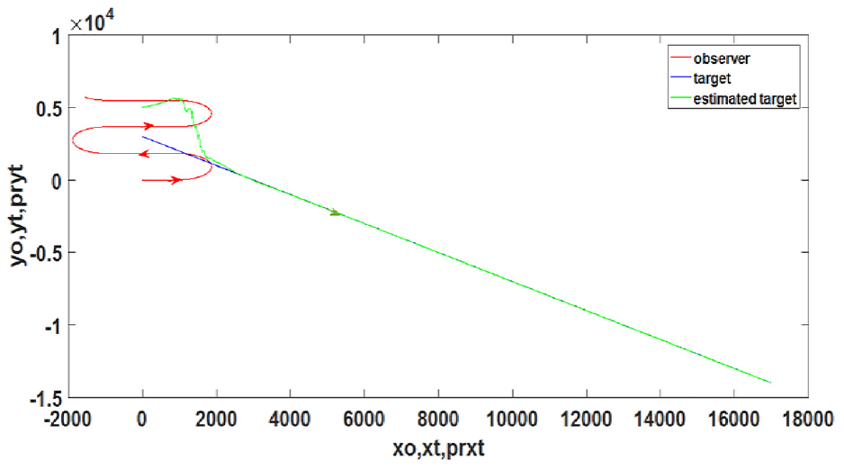
Observer and target path for scenario 1.
The algorithm is said to be converged in the range, course and speed, once the solution is accepted. This criterion is based on three-sigma error, that is, maximum error that can be allowed and this is expressed using SD in errors (one sigma) of TMP. Acceptance criteria for the given scenarios are as follows:
Range error estimate is ≤2.66% of the actual range.
Course error estimate is ≤1°.
Speed error estimate is ≤0.33 m/s.
Table 2 gives the convergence time of solutions which are executed for both DBEKF and DBUKF algorithms for low, medium and high ATB scenarios with Gaussian noise incorporated measurements. The convergence time for the low ATB scenario 1 with respect to range, course and speed are 1262, 484 and 1385 s, respectively, for DBEKF algorithm. Similarly, for DBUKF algorithm, the convergence times of low ATB scenario 1 for range, course and speed are 418, 338 and 465 s, respectively. The total convergence times for low ATB scenario 1 for DBEKF and DBUKF algorithms are 1385 and 465 s.
Convergence time in seconds for Gaussian noise.
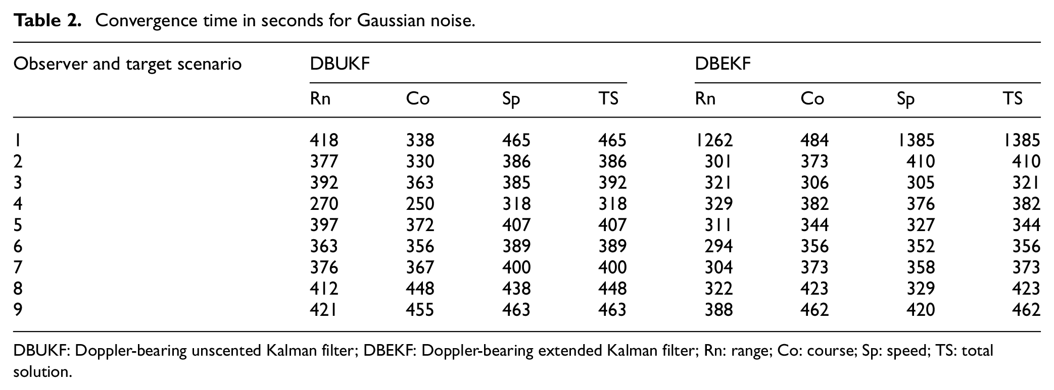
DBUKF: Doppler-bearing unscented Kalman filter; DBEKF: Doppler-bearing extended Kalman filter; Rn: range; Co: course; Sp: speed; TS: total solution.
The simulation results for 100 Monte Carlo runs are performed for low, medium and high ATB scenarios using MATLAB for both DBEKF and DBUKF algorithms. Convergence time obtained for 100 random shot noise samples with maximum noise amplitude of 2° for DBEKF and DBUKF is shown in Table 3. Similarly, the convergence time obtained for 400 random Gaussian mixture noise samples with maximum noise amplitude of 1.8° for DBEKF and DBUKF algorithms is shown in Table 4.
Convergence time in seconds for shot noise.
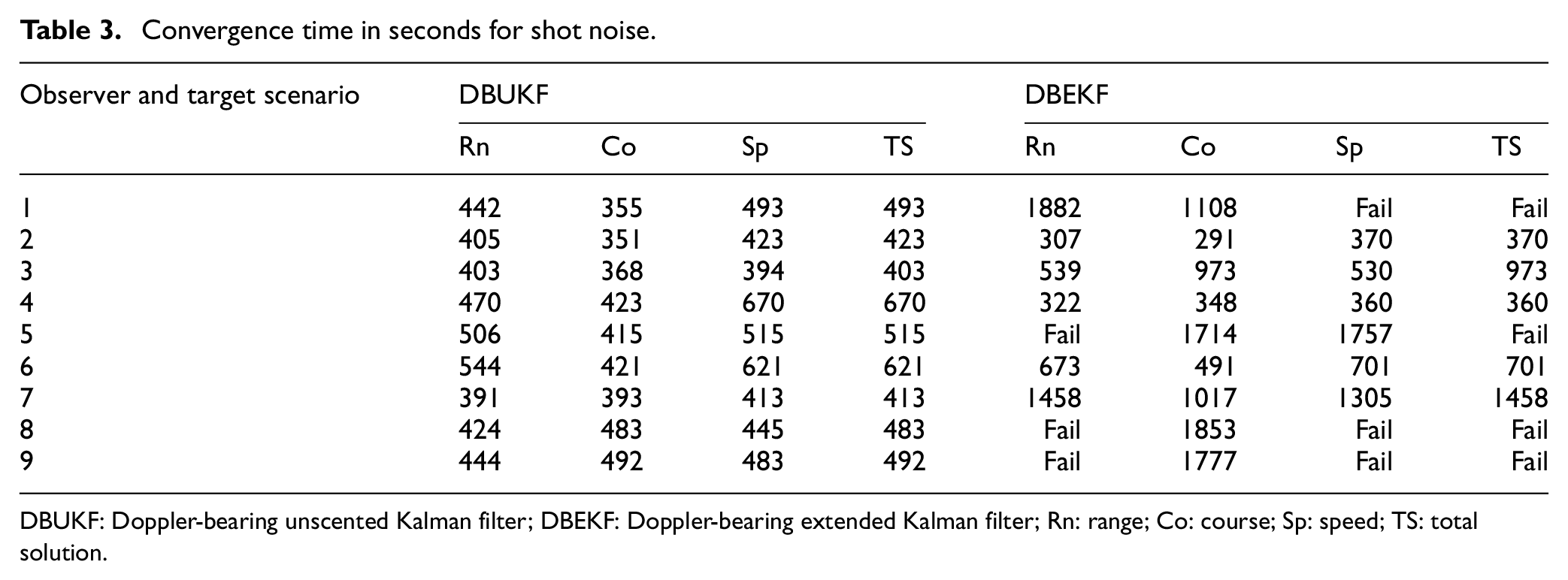
DBUKF: Doppler-bearing unscented Kalman filter; DBEKF: Doppler-bearing extended Kalman filter; Rn: range; Co: course; Sp: speed; TS: total solution.
Convergence time in seconds for Gaussian mixture noise.
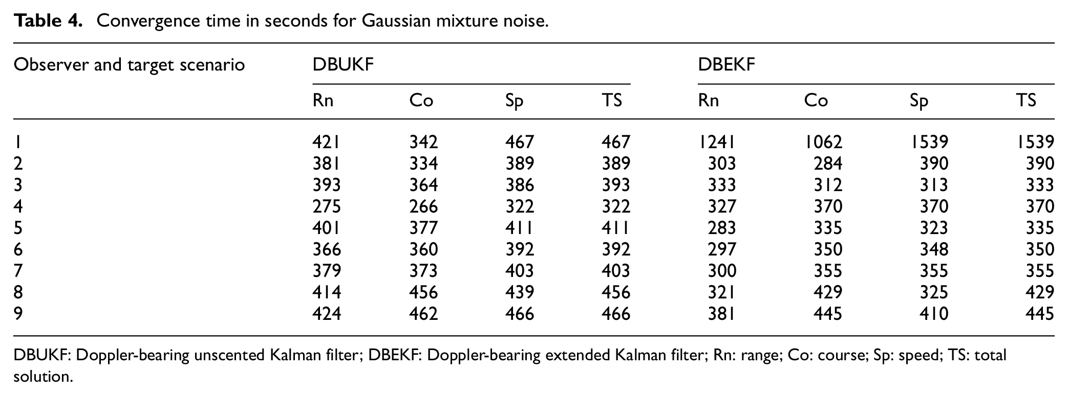
DBUKF: Doppler-bearing unscented Kalman filter; DBEKF: Doppler-bearing extended Kalman filter; Rn: range; Co: course; Sp: speed; TS: total solution.
In this paper, the scenarios in Table 1 are chosen to replicate the target tracking in real time. Speeds of observer and target are maintained as low as possible, as in real time submarines move at low speed to reduce the self-noise and also to avoid being tracked by the target. Target scenarios (based on course) are categorized according to ATB to determine whether the target is moving toward or away from the observer.
Till now, the performance of DBEKF and DBUKF is evaluated in Gaussian environment only and according to the literature, these two algorithms are not suitable in non-Gaussian environment. But in real-time scenario, the noise is a mixture of Gaussian and/or NGN and not completely non-Gaussian throughout the tracking process. Hence, a mixture of both Gaussian and NGNs is considered in this experiment to replicate real data analysis for tracking.
Root mean square (RMS) errors in estimated range, course and speed of the target in this paper are shown for scenario 1 of Table 1. Figure 6 represents the comparison of RMS errors for low ATB scenario 1 with Gaussian noise for DBEKF and DBUKF algorithms. Similarly, Figure 7 represents the comparison of RMS errors for the same scenario with shot noise for DBEKF and DBUKF algorithms. Figure 8 represents the comparison of RMS errors for the same scenario with the Gaussian mixture noise for DBEKF and DBUKF algorithms. The RMS errors in the estimated range are also compared with the theoretical CRLB as shown in Figures 6–8 for low ATB scenarios for all types of noises. It can be observed from the figures that the RMS errors of DBEKF are higher than that for DBUKF and for RMS range error. The RMS error values obtained for DBUKF are closer to CRLB than that of DBEKF proving DBUKF to be a better algorithm for tracking.
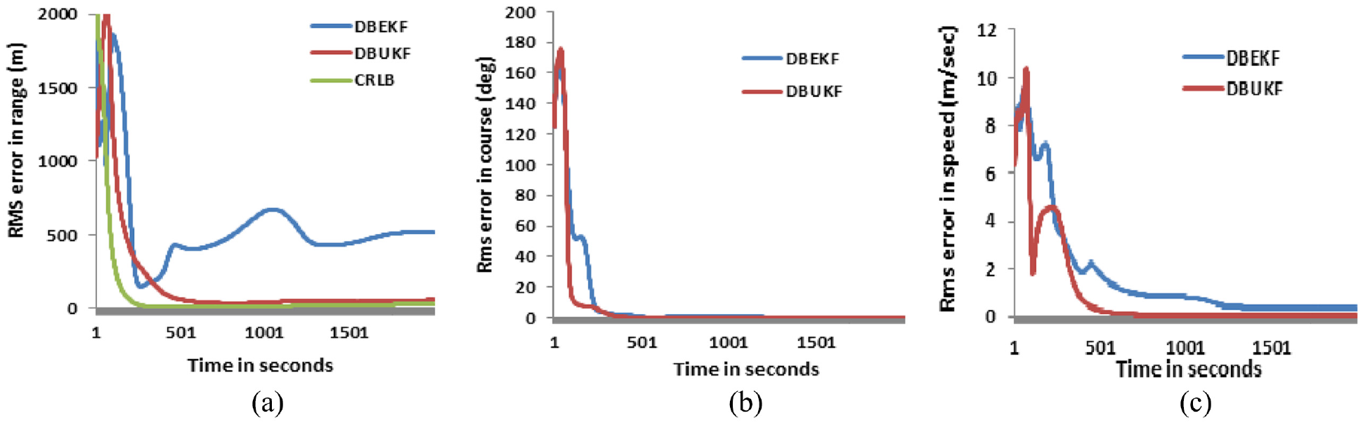
RMS error with Gaussian noise for low ATB scenario 1: (a) RMS range error, (b) RMS course error and (c) RMS speed error.
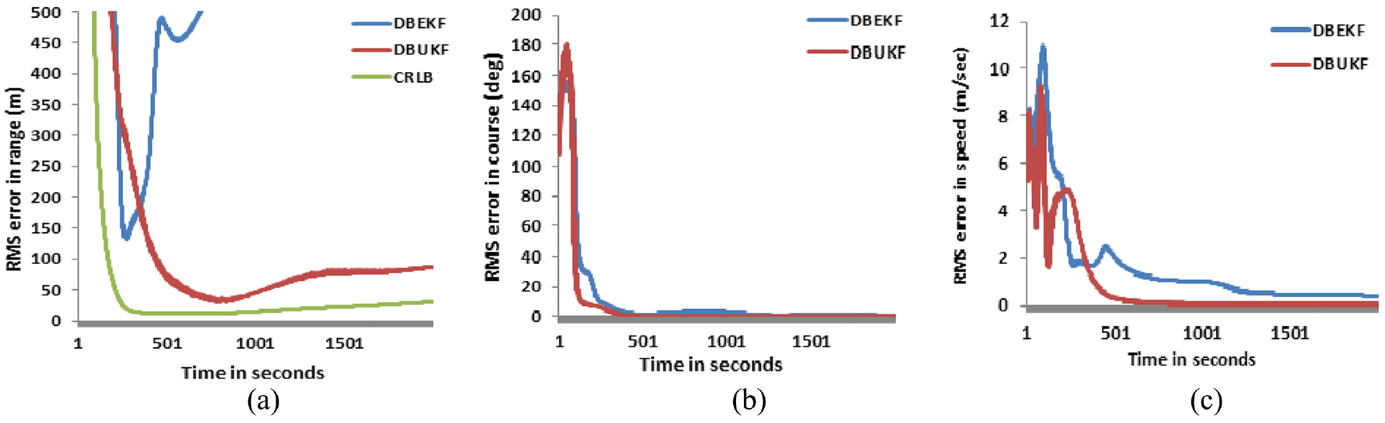
RMS error with shot noise for low ATB scenario 1: (a) RMS range error, (b) RMS course error and (c) RMS speed error.
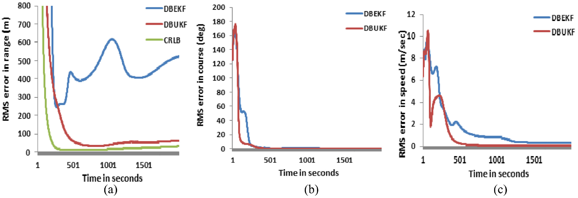
RMS error with Gaussian mixture noise for low ATB scenario 1: (a) RMS range error, (b) RMS course error and (c) RMS speed error.
DBEKF and DBUKF are not suitable for NGNs according to the literature.13–15 But in real scenario, the noise will not be non-Gaussian all the time. Therefore, taking NGN at certain samples, the algorithms are evaluated. In real-time scenarios, the convergence time should be obtained before 700 s. Taking this as the criteria, performance of the algorithms is evaluated for maximum noise amplitude of 3° in bearing measurement. With increasing nonlinearity, the DBEKF algorithm becomes unstable and the results cannot be predicted. Therefore, for DBEKF algorithm, the results are analyzed only for the scenarios with low nonlinearity.
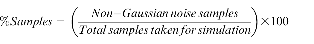
The algorithms can be performed under NGN only up to a certain extent. The percentage of samples that DBUKF can withstand for different NGNs is given in Table 5. Here, the occurrences of noise in measurements are taken in two patterns, namely continuous and random. The noise occurrence in measurements is said to be continuous if the noise occurring at continuous intervals of time. For example, if the noise in measurements is occurring at every third sample, then the noise occurrence is said to be continuous. If the noise occurs at random samples, then the noise occurrence is said to be random. The percentage of samples mentioned is calculated as follows
Percentage of samples with non-Gaussian noise that DBUKF can withstand.
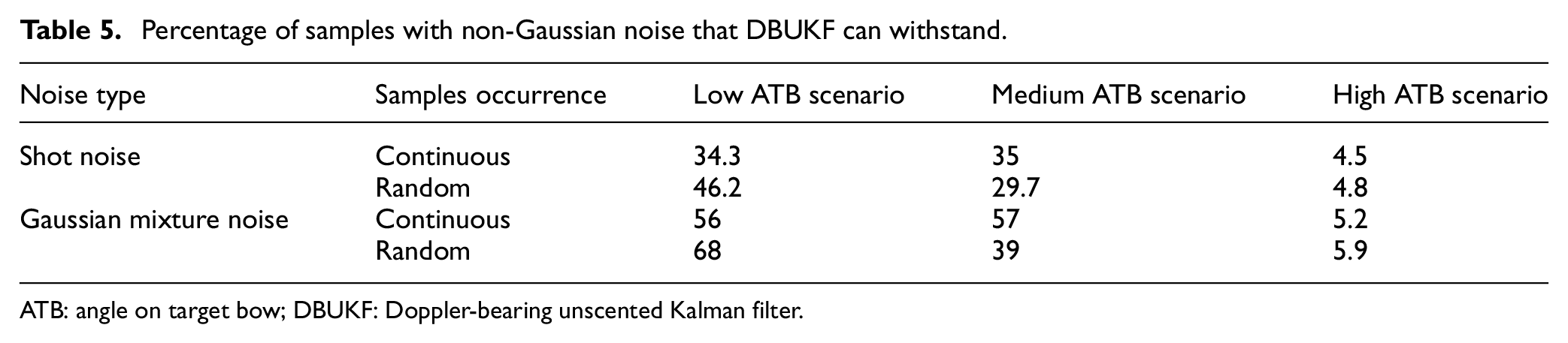
ATB: angle on target bow; DBUKF: Doppler-bearing unscented Kalman filter.
From the simulation results, it can be inferred that DBUKF can take up to 34.3%, 29.7% and 4.5% of samples with shot noise for low, medium and high ATB scenarios, respectively. Similarly, it can withstand up to 56%, 39% and 5.2% of samples with Gaussian mixture noise for low, medium and high ATB scenarios, respectively.
It can be observed from the convergence times given in Table 2 that for Gaussian noise, the solution is obtained for both the algorithms but for some scenarios DBEKF algorithm could not perform well. From Table 3, it can be observed that DBEKF algorithm fails in the presence of shot noise due to its instability as the noise amplitude increases. In the presence of Gaussian mixture noise, DBEKF algorithm performance is near to that as in the presence of Gaussian noise, as shown in Table 4. But as the noise amplitude and the non-Gaussian samples increase, the algorithm becomes unstable.
In real-time tracking, if the solution is not obtained within a stipulated time, then it is of no use as the observer may be at risk by the target. Hence, the performance of algorithms is evaluated based on the convergence time of the solution within 700 s.
Figure 9 represents the comparison of different noise types with respect to CRLB in terms of RMS errors in range, course and speed of the target. It can be observed from the figure that in the presence of Gaussian noise, the estimation errors are low and nearer to CRLB than other types of noises. In the presence of Gaussian mixture noise, the RMS errors in the estimation of TMP are much closer to that in Gaussian noise environment. Hence, the performance of filter in Gaussian mixture environment is similar to that in the presence of Gaussian noise. The RMS errors in estimated TMP are more when compared to other types of noises. Hence, in a shot noise environment, the filter performance is not as efficient as in Gaussian or Gaussian mixture environments.
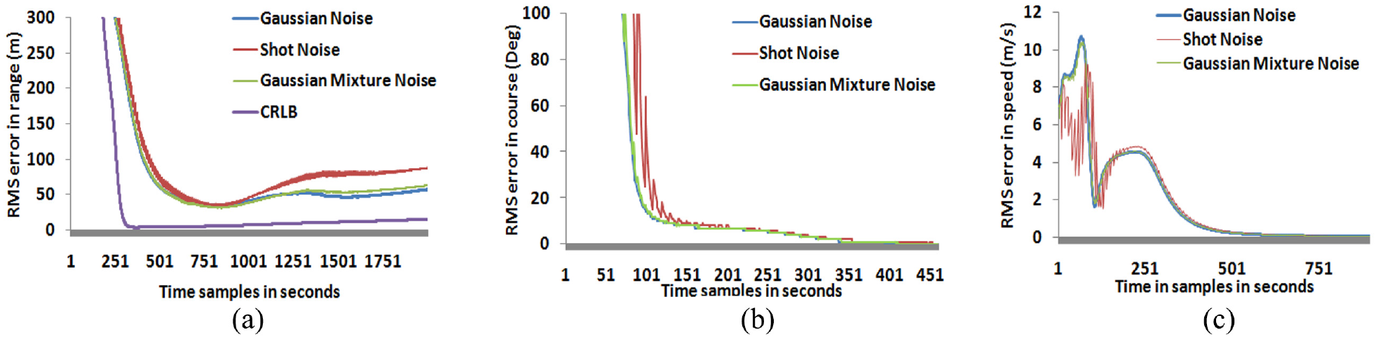
RMS error for different noises using DBUKF for low ATB scenario 1: (a) RMS range error, (b) RMS course error and (c) RMS speed error.
Conclusion
In this paper, the effort is made to analyze both DBEKF and DBUKF algorithms in the existence of Gaussian noise and two different non-Gaussian disturbances. The results show the efficiency of DBUKF and DBEKF in the presence of different types of noises. DBEKF algorithm is highly unstable as the noise in measurement increases, and also with an increase in nonlinearity in scenarios chosen; hence, the percentage of samples that DBEKF can withstand cannot be determined. As the ATB increases, target moves away from the observer; hence, the percentage of samples that DBUKF algorithm can withstand decreases as the range increases. Therefore, it is clear from the simulation that DBUKF has better stability than DBEKF. It was observed from the simulation results that DBUKF works well with both types of noises while DBEKF works only under certain limitations. DBEKF algorithm is highly unstable as the noise increases. Hence the percentage of samples that DBEKF can withstand cannot be determined. As the ATB increases, the target moves away from the observer; hence, the percentage of samples that DBUKF algorithm can withstand decreases as the range increases. However, with limited noise samples, DBUKF exhibits consistent results than DBEKF.
Footnotes
Declaration of conflicting interests
The author(s) declared no potential conflicts of interest with respect to the research, authorship and/or publication of this article.
Funding
The author(s) received no financial support for the research, authorship and/or publication of this article.