General model for best feature extraction of EEG using discrete wavelet transform wavelet family and differential evolution

Abstract

Wavelet family and differential evolution are proposed for categorization of epilepsy cases based on electroencephalogram (EEG) signals. Discrete wavelet transform is widely used in feature extraction step because it efficiently works in this field, as confirmed by the results of previous studies. The feature selection step is used to minimize dimensionality by excluding irrelevant features. This step is conducted using differential evolution. This article presents an efficient model for EEG classification by considering feature extraction and selection. Seven different types of common wavelets were tested in our research work. These are Discrete Meyer (dmey), Reverse biorthogonal (rbio), Biorthogonal (bior), Daubechies (db), Symlets (sym), Coiflets (coif), and Haar (Haar). Several kinds of discrete wavelet transform are used to produce a wide variety of features. Afterwards, we use differential evolution to choose appropriate features that will achieve the best performance of signal classification. For classification step, we have used Bonn databases to build the classifiers and test their performance. The results prove the effectiveness of the proposed model.

Introduction

Brain–computer interface (BCI) is a direct channel of communication between brain and the computer, ¹ and this contact is used by computer to control brain. The research started in the field of BCI in 1970s in the University of California, Los Angeles. ² The focus was on artificial neural limbs that participate in applications, which aimed to restore defect in hearing, sight, or movement. The basic idea of BCI principle depends on four main steps. First, getting the information or brain waves (signals). Second, electroencephalogram (EEG) processing by filtering signals from sources other than brain, and unwanted signals are produced either from vital sources, such as eye muscles movement, or from external sources, such as the movement of electrodes or electrical appliances. Usually, noise is determined by filtering the electrical signals depending on frequencies. Third, extracting features; this step converts signals that are received in a specified time from several channels to many features that are easily categorized by tasks. This step relies on different algorithms for extracting and classifying features. Fourth, controlling the machine; in this step, the computer sends a signal to machine that user wants to control based on its classification of features from earlier step. The steps are summarized in Figure 1.

Figure 1.

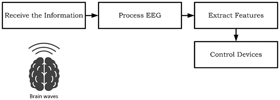
BCI principle.

The EEG is a unique and important measure for evaluating the function of brain like an electric scheme that shows difference in electrical voltage between any two locations on brain recorded over a period. It is possible to obtain from different frequencies which appear according to the type of stimuli, whether physical, chemical, or mechanical. Then it is possible to assess the response of regions which are responsible for any type of stimuli and to identify ideal areas of sensitivity via five senses (smell, taste, vision, hearing, and touch) using diagrams that record displacement value of voltage groups according to response of different regions in receiving and resulting electrical effect. There are different regions in brain that respond to a stimulant. It is chemically sensitized by smell or taste, mechanical stimuli by dragging and touching, and so on. This research focuses on the classification of different brain signals using artificial intelligence algorithms after extracting least number of information from EEG signals to ensure high accuracy of classification with reasonable performance.

In this study, a computer-aided EEG analysis method was introduced to obtain a highly efficient seizure detection method at high accuracy and low-cost levels. There are four main factors which have a direct impact on discrete wavelet transform (DWT) performance, summarized by: DWT coefficient feature, mother wavelet, and frequency band and decomposition level.

This article includes four main sections divided as follows: section “Related Works” addresses previous works associated with our study. Section “Proposed Classification Model” describes the details of proposed classification method. Section “Data sets description” describes the data set used in our study. Section “Results and discussion” presents the results and their justifications, and finally we conclude our work in section “Statistical analysis.”

Related works

EEG signal is a method used to record the electrical activity of brain over a period in order to diagnose many kinds of diseases such as epilepsy, Alzheimer, and Schizophrenia. In addition to the usage of EEG in diagnosis of diseases, it is widely applied in many fields like cognitive science, neurolinguistic researches, neuroscience, psychophysiological research, and cognitive psychology.^3,4

Over the years, many EEG classification models have been presented, despite insufficient similar extent in the comprehensive evaluation of these models on domain-specific health applications. Different health domains have very different demands for their classification accuracy, but in general, not all machine learning models will be suitable for every application. In this section, we briefly explain some recent studies that are related to EEG classification and preprocessing.

EEG signal is used to detect emotions of human such as sadness, happiness, and many other emotions using psychological factors or facial and voice gestures. The process of detecting emotions can be achieved through recording brain activity for a period and discover patterns to relate it to emotional states.

In order to detect if the patient is in a non-convulsive status epileptics, the physicians used EEG to decide the best treatment based on the diagnostic level of EEG test. The following are three conducted types of research that used EEG signals to diagnose epilepsy.

Ibrahim et al. ⁵ proposed an adaptive learning model for epilepsy diagnosis based on EEG signals. In features-extraction step, they used discrete wavelet transform (DWT) and Shannon entropy. While in classification step, the nearest neighbor was used to classify signals into two categories that are normal and epileptic. For the experiments, they used standard Bonn database. To evaluate the performance of model, three common evaluation measures were used which are sensitivity, specificity, and accuracy. It achieved 100% with the three measures when setting A and 97% with the whole database.

Another research was proposed by Sharma et al., ⁶ where the authors suggested a novel automatic pattern to identify epileptic seizures based on two common techniques which are analytic time-frequency flexible wavelet transform (ATFFWT) and fractal dimension (FD). The proposed model used several important features, which are flexible time-frequency, shift-invariance property and tunable oscillatory attribute. These features are suitable when signals are unstable and transient. EEG signals decompose into the desired sub-bands based on ATFFWT. Then FD is used for each sub band. The last step is to use the classifier of least-squares support vector machine (LS-SVM) for outputs of sub-bands FDs. Their proposed model had achieved satisfying results with (sensitivity = 100%) with (10-fold) cross-validation.

A number of EEG classification models based on parameters modifying, such as probabilistic neural network, SVM, and ensemble of machine learning classifiers, have been successfully used to classify signals to determine epilepsy patients. Satapathy et al., ⁷ in their study, proved that ensemble model outperformed recurrent neural network in terms of accuracy and time complexity with 99.5% and 3.745 s, respectively. To conduct their experiment, they used a publicly available database from Bonn University. This data set provided five subsets with 100 subjects for each. It is worth mentioning here that they used DWT for feature extraction step.

Truong et al. ⁸ assessed the accuracy of random forest (RF) using automatic channel selection (ACS) for preprocessing of EEG signals. After that, they extracted features using Hills’ algorithm, where the features contain spectral power with (1 Hz) bins and eigenvalues. They conducted their experiments using the data set of four dogs and eight patients with epileptic seizures. Their results proved the efficiency of their proposed method with (91.95%) sensitivity and (94.05%) specificity.

Amin et al. ⁹ applied the discrete wavelet transform on EEG signals and calculated the relative wavelet energy in terms of detailed coefficients and approximation coefficients of the last decomposition level. The EEG data set employed for the validation of the proposed method consisted of two classes: (1) the EEG signals recorded during the complex cognitive task—Raven’s advance progressive metric test and (2) the EEG signals recorded in rest condition—eyes open. The performance of four different classifiers was evaluated with four performance measures, that is, accuracy, sensitivity, specificity, and precision values. The accuracy was achieved above 98% by the SVM, multi-layer perceptron (MLP) and the k-nearest neighbor (KNN) classifiers with approximation (A4) and detailed coefficients (D4), which represent frequency range of 0.53–3.06 and 3.06–6.12 Hz, respectively.

There is no doubt that preprocessing is an important and essential step for any system based on the signal. Several recent studies have tried to find a better method to process EEG signals like the study that was presented by Gregory et al. ¹⁰ They proposed a new approach to process (EEG) signals. They utilized two methods, which are: event-related de-synchronization (ERD) technique and event-related synchronization (ERS) technique. These techniques were used to increase the speed of motor imagery movements. Their proposed approach takes into consideration the specific time intervals, based on the requirements of control of brain in real time of rehabilitation equipment, which led to facilitate the command and control of these devices based on patient’s will. Their model passes through two basic steps: the first step is removing noise, which is produced from overlap with normal human activities such as cardiac movement and eye blinking. The second step is using SVM classifiers to classify the signals that have been processed (energy features based) according to the signals available in database. The results proved that this approach achieved good results in terms of complexity of time and accuracy.

The EEG signals produce a huge amount of redundant data, which highly affect the process of EEG analysis. Amin et al. ¹¹ propose to use this redundant information of EEG as a feature to discriminate and classify different EEG data sets. They proposed a JPEG2000-based approach for computing data redundancy from multi-channels EEG signals. They used the redundancy as a feature for classification of EEG signals. The approach is validated on three EEG data sets and achieved high accuracy rate (95%–99%) in classification.

In the research that was published in 2016, Gopan et al. ¹² applied several statistical features to classify Eyes Open (EO) and Eyes Closed (EC) relaxed states, which were used as a baseline for EEG analysis. In addition, they used SVM and KNN as classifiers. The research focused on the importance of choosing suitable baseline for any EEG analysis in order to get lowest level of activation in an experiment and emphasized that brain-machine interface requires a suitable baseline for each function. The research concluded that the best accuracy (77.92%) was obtained when three algorithms were combined with KNN classifier (K = 7). These three algorithms include Kurtosis, mean absolute deviation (MAD), and interquartile range (IQR). This combination emphasized the importance of data distribution in characterizing two states.

Some researchers have explored different types of statistical and machine learning models for EEG classification. For example, the study Radüntz et al. ¹³ implemented SVM and artificial neural network (ANN) for classification step. They have been adopted in several stages. These stages started with the preprocessing of EEG signals to extract features from them and then combining these features as vectors. The process ended by classifying these vectors. The aim of this study was to exclude artifact EEG signals that are affected by humans. These were the results of several biological causes, such as eye movements and muscle activities. They used independent component analysis (ICA) as a preprocessing step. They relied on two classification algorithms, SVM and ANN, where their results showed that the use of ANN was better than SVM in terms of accuracy, with 95.85% and 94.04%.

There has been more than one version of SVM algorithm for supervised learning. These versions obtained based on the parameters modifying, which include soft SVM, LS-SVM, hard E-SVM, and rLS-SVM. ⁶ Patidar S and Panigrahi ¹⁴ concluded that LS-SVM performs well with five standard data sets, but by using the tunable-Q wavelet transform (TQWT) and the Kraskov entropy, this assumption does positively affect the results. Those results were like this; accuracy: 97.75%, sensitivity: 97.00%, and specificity: 99.00%.

Zhang et al. ¹⁵ proposed a new pattern for EEG signals classification and illustrated two types of EEG signals for feature-extraction methods. For the first method, the autoregressive (AR) model and approximate entropy are combined, while in other method, AR model is combined with wavelet packet decomposition (WPD). The purpose of their research is using a combination of methods in order to modify acquired EEG signals into feature vectors, then, classify those vectors using SVM classifier, which is used after feature extraction process. In addition, an experiment of validation is used. The research concluded that the technique of feature extraction, which combines the WPD and AR model, does a better performance than other method in mental function. Experiment validated this conclusion. Their research was published online in 2016.

Manjusha M and Harikumar ¹⁶ used k-means clustering and KNN classifier in their model of EEG signals for the classification process. At the data collection stage, they recorded EEG signal to twenty patients, then applied Detrend fluctuation analysis for determining non-linearity present in the database followed by a step of dimensionality reduction based on power spectral density technique. Finally, KNN and k-means were implemented for categorizing EEG signals. The proposed model achieved satisfactory results of sensitivity and specificity of 78.31% and 93.02%, respectively, with k-means. While it achieved 90.4878% and 92.8475%, respectively with KNN.

A wide variety of techniques were used for the extraction and classification of EEG signals. In general, most of the techniques passed through four main steps which are as follows: noise removal, feature extraction, feature selection, and classification of the resulted features. Fernández-Varela et al. ¹⁷ used two different machine learning combinations based on six models: ANNs Fisher’s linear discriminant, SVMs, KNN Trees, and Naive Bayes. The first proposed approach was built depending on short life and Buchanan’s certainty factors, and the second approach depended on linear combination of two models. They conducted their experiments using two data sets with 20 and 26 recordings. In both approaches, the proposed method was divided into processing phase and classification phase. The first phase started by elimination of artifacts signals, blocking signals, and group intervals. While machine learning phase extracted features and classified signals, using individual and hybrid models. Their results showed that the first approach achieved sensitivity of 0.78 and specificity of 0.89, while the second approach achieved sensitivity of 0.81 and specificity of 0.88%.

Hassan and Bhuiyan ¹⁸ proposed a new approach for the computerized sleep staging method. This approach is based on TQWT to detect EEG single channel. At the beginning, their proposed model started with disbanding signal segments into sub-bands of the sleep EEG signals. After that, the pdf modeling of normal inverse Gaussian (NIG) was applied for extracting the features and then adaptive boosting (AdaBoost) was used for classification step. The experiments used 10-fold cross-validations for evaluating the performance of the approach. The results were evaluated using four popular measurement techniques: accuracy, sensitivity, Cohen’s kappa coefficient, and specificity. Vincent’s University Hospital/University College Dublin sleep apnea database was used for experiments. The model achieved good results, where Cohen’s kappa coefficient outperformed the rest with 0.82 (6-Class), 0.818 (5-Class), 0.93(4-Class), 0.965(3-Class), and 0.99 (2-Class). Table 1 summarizes some related studies.

Table 1.

Examples of related studies.

Authors	Year	Used data set	Modeling technique	Findings	Feature extraction	Limitations
Satapathy et al. 7	2017	Five sets of EEG signals. Each set contains a reading of 100 single-channel EEG segments of 23.6-s duration each	SVM and ANN ensemble	Case 1 (set A and E): 99.5% Case 2 (set D and E): 99.5% Case 3 (set A + D and E): 98.3%	DWT	Ensemble restricted to voting, using of DWT which resulted in high complexity time
Radüntz et al. 13	2017	set1: 57 set2: 12 set3: 10	SVM and ANN	ANN with an accuracy of 95.85% SVM: 94.04%	Independent component analysis (ICA)	Time-consuming computation of the ICA
Truong et al. 8	2017	Data from four dogs and eight patients with epileptic seizures	Random forest	91.95% sensitivity and 94.05% specificity	Automatic channel selection (ACS) for preprocessing Hills’ feature extraction algorithm	High accuracy of RF needs more trees which imply more computational time
Fernández-Varela et al. 17	2017	20 Recordings 26 PSG recordings	Fisher’s linear discriminant, SVM, ANN, DT, KNN, and NB	First approach: a sensitivity of 0.78 and a specificity of 0.89 Second approach: a sensitivity of 0.81 and a specificity of 0.88	Hjorth’s parameters for sleep stage	The study deals with the original signals without noise removal. Also, no dimensionality reduction method was used
Patidar and Panigrahi 14	2017	Five subsets: Z, O, N, F, and S forms the whole data. Each subset contains 100 single-channel EEG signals	LS-SVM	Acc.: 97.75, Sen.: 97.00, Spec.: 99.00	The tunable-Q wavelet transforms (TQWT) represents the sparsity in signals Kraskov entropy with Euclidian distance	The Lagrangian multipliers for the LS-SVM tend to be all non-zero
Sharma et al. 6	2017	Five subsets: A, B, C, D, and E. The two sets of A and B have EEG data which was recorded from five healthy subjects	LS-SVM	Sensitivity = 100%	Signal decomposition: using ATFFWT FE: Computation of fractal dimension (FD)	To calculate the FD’s features of the signal, there is a restriction in computing the total waveform length to the window size to be used
Mehmood and Lee 19	2015	LAPS database	SVM and KNN	Best accuracy was 61%, which was acquired by KNN (k = 3)	Hjorth parameters that were used in feature extraction of all channels of EEG at each epoch	The accuracy is not good compared to other studies, the combination of 2 or 3 feature extraction methods may result in better accuracy percent
Ibrahim et al. 5	2016	University of Bonn EEG data set	Adaptive KNN Baseline	Accuracy = 100%	A combination of DWT and Shannon entropy	The accuracy of KNN strongly depends on data size, thus, the results are not stable. DWT has high computational complexity
Manjusha and Harikumar 16	2016	20 epileptic patients who were under examination and medication in the neurological department of Sri Ramakrishna Hospital, Coimbatore.	KNN k-means clustering	KNN: 78.31% k-means clustering: 93.02%	Dimensionality reduction: power spectral density	KNN affected accuracy negatively
Hassan and Bhuiyan 18	2017	Sleep-EDF database which is available in Physio net. No. of epochs = 15188	(AdaBoost) with 10-fold cross-validation	Accuracy = 98.56 with 2-classes	TQWT transform. NIG parameters are used as features	AdaBoost can be sensitive to noisy data and outliers

Proposed classification model

In this article, we proposed a new approach based on a hybrid of wavelet family and differential evolution (DE) for recognition of epilepsy cases from EEG signals. First, we used the standard raw EEG signals that are available in Bonn University where our approach composes of four main steps: preprocessing, feature extraction, feature selection, and classification.

Feature extraction

Due to electromagnetic interference between high frequency, which is generated from the oscillators and low frequency from eye blinks and muscle stretching, we conclude that EEG time series signals are none-stationary, since it includes much information with both frequencies.

The capability of capturing the frequency information, during brain activities is difficult to be obtained. ²⁰ To solve this problem, we need an efficient approach toward those signals in such a way which gives more accurate and specific data analysis. ²¹ For this issue, we use wavelet transform (WT), which is considered as one of the techniques that uses multi-resolution analysis that divides the signals into different frequency spectrums. Also, WT combines high- and low-frequency spectrums.

Dealing with raw signals affects the accuracy results negatively. Therefore, identifying noises and removing potential ones from EEG signals are a major step in the analysis of the raw data. Rejecting experiments and trial with noises is one of the other traditional methods, which involve the design of some experiments to allow this eventuality. In related work, some methods have been employed to remove noise by almost all experts. A brief description of noise removal techniques, which should be followed from the methods used in the EEG, will be presented.

The ICA algorithm is one of the most used statistical techniques used in the field of signal noise removal, especially EEG signals. Many of the related studies have used ICA to correct or remove contaminants in brain wave planning.^22,23 The aim of this technique is to reduce the influence of surrounding factors in the form of EEG signals. It is one of the most prominent source separation techniques, which usually assumes varied normal and behavior of the EEG signals. Thus, it depends on the construction of an automatic way to re-represent signal with separation of deformation. So that it produces a clean reading of the brain planning by zeroing the weights of unwanted segments.

The importance of using this method lies in its strength in dealing with the nature of EEG signals, as it suffers from severe noise at central poles, especially in the range of gamma above 20 Hz, which are considered as strongest contaminants. In this article, we applied this method to the raw data to minimize the noise that negatively affects the performance of signal classification systems. ²⁴

The advantage of feature extraction is to enable us to automatically choose for the optimal group of attributes in the original data. ¹² The problem to be resolved is the key to determine the degree of preference of most suitable subset of attributes. But overall, we mean the most precise set. The feature-extraction method is used to give new subsets for features while evaluation metrics record different subsets. The best technique is the simplest one and is based on testing features in each subset to get lowest rate of errors. It is comprehensive and easy to calculate but gives good results for small sets. The algorithm is heavily influenced by evaluation scale used to distinguish following types: wrappers, embedded methods, and filters.

The epileptic seizure signal includes two kinds of EEG time-based frequencies, high-frequency information with short period and low-frequency information with long time periods. ²⁵ The use of WT can work continuously (CWT) or discrete (DWT) that is used in our article. One of the disadvantages of CWT is redundancy, whereas DWT is more efficient due to the frequency filter bank, which is used to remove the unwanted frequencies and decompose the signal into diverse levels using five levels of decomposition, each one contains the sample decomposed by two components.

There are many types of DWT, which are considered as mathematical and statistical functions. These types were divided to families according to frequency components. ²⁶ Leading step in wavelet-based digital signal processing (DSP) depends on the choice of the appropriate mother wavelet. Multiple mother wavelets result in different degrees of DWT in the same EEG segment, which eventually leads to multiple detection results. Seven different types of common wavelet were tested in our work. These types are Discrete Meyer (dmey), Reverse biorthogonal (rbio), Biorthogonal (bior), Daubechies (db), Symlets (sym), Coiflets (coif), and Haar (Haar). Figure 2, shows all the DWT types.

Figure 2.

Wavelet types.

DWT has been very effective in our proposed model. Wavelet is known as a fast-fading function with oscillating frequency bands and oscillating time as well. ²⁷ The CWT are analyzed into two parameters; scaled and translated. The formula is representing one function below (mw x, y (s)) and mother wavelet mw (s)

$$m{w}_{x,w}=\frac{1}{\sqrt{|x|}}\mathrm{mw}\left(\frac{s-y}{x}\right)$$

(1)

where scale parameters are represented by x, and y is the translation parameter with x, y∈ℝ, such that x is equal to a non-zero value, and by discretizing these parameters, the DWT is obtained. ²⁸ Often, DWT is used as a dyadic sample with parameters x and y which depends on the power of x = 2j and y = k*2j, with j, k∈ℤ and by replacing them with formula (1), which results in waves ¹⁸

$$m{w}_{j,k}=\frac{1}{\sqrt{|2^j|}}\mathrm{mw}(2^{-j}s-k)$$

(2)

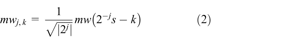
As DWT is given by the following formula²⁰

$$d_{j,k}=\underset{-\infty }{\overset{+\infty }{\int }}r(s)2^{-j/2}*\mathrm{mw}*(2^{-j}s-k)\mathrm{dt}$$

(3)

$d_{j,k}$ represents the wavelet coefficients, where k denotes location, and j denotes level. In our approach, feature extraction depends on these coefficients to build the vectors for each EEG signal in the detection of seizures.

We have used DWT to extract the features because it is a very effective method compared to other methods in terms of accuracy of extraction features to ensure the effectiveness in the following steps, this had been proved in several previous studies such as Li et al. ²⁹ and Prochazka et al. ³⁰

The main characteristic of DWT which makes it one of the best methods for the analysis of EEG signals is its resolution of frequency and time. This property leads to optimality status for frequency–time resolution. ²⁶

The process starts with the first signal that goes into a band-pass filter. Band-pass filter is a combination of both high-band-pass filter (HPF) and low-band-pass filter (LPF) to have the requested result. This process is categorized as the first level, which includes two corresponding coefficients; one of them is Approximation (A) and the other is Detailed (D), since it is categorized under the first level, it will be denoted as A1 and D1 and the process goes on under multiple levels as a subsequent of coefficient from the first level within the approximation, for example (A2, D2) and (A3, D3). At each process, the frequency resolution is doubled using the filters while decomposed and reduced the time complexity to half. We used the DWT to extract features, where it was applied to five levels and the features as follows D1, D2, D3, D4, D5, and A5. After getting these features, we then apply a statistical formula in the next section. Thus, the results of applying the statistical functions are 2184 features for each signal, in addition to the class name (normal/seizure), the total number of features are 2184 (6 wavelet coefficients × 52 mother wavelets × 7 features).

Statistical features

It is important to select the appropriate features in the EEG classification, which can find the best features for EEG signals. The feature vector of the EEG signal is formed by several occurrence bands that produce DWT coefficients. In this work, considering equation (3), DWT coefficients are calculated from the EEG segment in each band. The EEG segment is built based on a pair of statistical features, as well as, seven wavelet features according to wavelet-based EEG signal processing. To extract the features from each DWT output factor, we used seven statistical functions, including mean absolute value (MAV), average power (AVP), standard deviation (SD), variance, mean, skewness, and Shannon entropy. We have adopted Shannon entropy functions in this study from a variety of entropy functions.

$$\mathrm{MAV}=\frac{1}{s}\sum _{i=1}^s\left|\mathrm{xi}\right|$$

(4)

$$\mathrm{AVP}=\frac{1}{s}\sum _{i=1}^s{\left|\mathrm{xi}\right|}^2$$

(5)

$$\mathrm{Var}=\frac{1}{s-1}\sum _{i=1}^s{(\mathrm{xi}-\mu )}^2$$

(6)

$$\mathrm{SD}=\sqrt{\frac{1}{s-1}\sum _{i=1}^s{(\mathrm{xi}-\mu )}^2}$$

(7)

$$\mathrm{Mean}=\frac{1}{s}\sum _{i=1}^s\mathrm{xi}$$

(8)

$$\mathrm{Skewness}=\frac{\sum _{i=1}^S{(x_i-\mu )}^3}{s*S{D}^3}$$

(9)

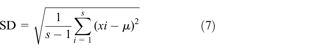
where x_i is the ith sample of EEG data in a segment, µ is the mean of the segment, and S is the length of the segment. ²¹

The Shannon entropy value is calculated for X = x₁, x₂,…, x_N, as in the next formula^22,31

$$H=-c\sum _{i=1}^{s}P\left(x_i\right){\log }_2\left(P\left(x_i\right)\right)$$

(10)

where S is the total of distinctive values in the data (x), while p_i represents the possibility of S values. C is a positive constant. Figure 3 shows this step.

Figure 3.

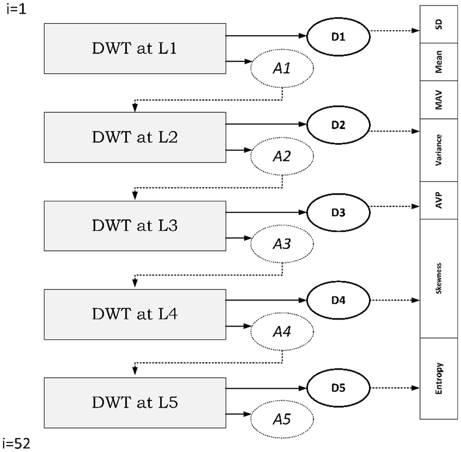
Feature-extraction step.

Feature selection

The next step is to select features, and this step depends on features that were extracted in previous step. We have applied previous statistical functions. We used evolutionary differential for selecting features for each signal, in addition to the class name (normal/seizure). The use of feature selection methods results in several benefits such as: ³² minimize the time needed for training stage—this makes training process work faster by reducing the processed data; reduce the amount of useless data—these types of data always shared error decisions; and raise the level of accuracy by clearing data.

The computer’s brain interface signals, which are used for the communication process, are very high in terms of features and size, which reflects negatively on the system performance. To resolve this problem, we use dimensional reduction techniques or so-called feature-selection algorithms, where these algorithms are used for choosing a subset of best features to improve system performance. The primary motivation for such algorithms is to reduce the size of dimensions and exclude recurring or non-system-related features and reduce number of features needed to learn system. This step reduces the complexity of computational processes that are required for system, thereby increasing the speed of system missions. ²⁹

As a result, a set of algorithms has recently appeared, known as approximate algorithms that obtain acceptable solutions, but not necessarily optimal solutions. These algorithms were designed to save time and effort because classical algorithms may need tens of years to solve some problems of systems improving when it deals with big data. Among these algorithms, we find that the most popular, with encouraging results are genetic algorithms, industrial neural networks, and differential evolutionary algorithms. The last one is considered as one of the best algorithms in terms of efficiency as a feature-selection algorithm.

Evolutionary methods

Evolutionary is one of the most widely used techniques for selecting best combination of features among many extracted features. These techniques have many different methods such as DE, simulated annealing (SA), particle swarm optimization (PSO), artificial bee colony (ABC), and ant colony optimization (ACO), the used one here is DE. Deferential evolution (DE) is defined as population algorithms like genetic algorithms, where they depend on the factors of mutation and crossover as well as selection. The main difference between two algorithms is that genetic algorithm relies more on crossover process while differential evolutionary algorithm focuses on mutation stage, which is represented in perturbation of genes with the difference between two other randomly chosen genes from the group.^26,33 This technique is a vector-based random search method. It has a strong affinity property, which means their ability to self-organize without the need to extract derived information, where it relies mainly on two operators: crossover and mutation.

The cycle of the DE method is composed of four main steps: ³⁴ (1) create a population of variable vector search in the initial case in which the population size is set to 50 and total 100 iterations are used, (2) Mutation, (3) crossover, and (4) selection. Mutation stage is utilized as a search method in DE algorithm, whereas selection is used as director of the search in the whole region. Finally, the crossover is used in solutions intersection phase, ²³ where Steps 2, 3, and 4 include the repeating of solutions generation until the stop criterion is met. The operation to use DE is briefly summarized as follows:

• Step 1: Initialization

First, the representation of any problem is a complicated issue in evolutionary algorithm, in case of genetic and differential types because this is a basic step to understand problem and to obtain an efficient algorithm in terms of results and complexity time. The initial phase includes generation of random vectors (N–1), where N is the number of chromosomes.

For our study, the space of given solutions depends on extracted features and that each of extracted features is used to build solutions. Therefore, the problem is formulated and represented from this final system with the aim of achieving highest value of performance measures based on confusion matrix elements, which are TP, TN, FP, and FN. These four values are obtained as a result of comparing the results of similarity between signals by relying on each individual feature. In order to reduce the number of features extracted in the previous step, a wrapper feature selection method is used. DE is initialized with a set of chromosomes in which each represents a candidate solution. The length of each chromosome is 2184 gene. Each gene represents a feature where the value of 1 means that the feature is selected and 0 means that the feature is not. As depicted in Figure 4, the data set is represented as two-dimensional matrix where columns are the features and rows are the signals. For each chromosome, the matrix is modified by deleting the columns that are mapped to zeros in the current chromosome. The resultant matrix is then used by KNN to evaluate the fitness of the current chromosome by evaluating the accuracy of the test data depending on the selected features

Figure 4.

Description of the evolutionary methods used with the data set.

Therefore, the fitness function is the highest value of TP and TN, which is intended to be efficient in classifying infected cases from healthy ones.

• Step 2: Mutation

In this step, new different vectors are generated, based on calculating the difference between two vectors to the third one. V_i in the jth iteration can be calculated using the following formula ³⁵

$$V_i,G+1=X{a}_1,G+F.(X{a}_2,G-X{a}_3,G)$$

(11)

where a₁, a₂, and a₃ represent three distinct random references belong to {1,2,…, NP}. F is a constant that increases the difference between the vectors.

In our case, we find the best solution, and this is simply done by ordering the results in terms of the highest TP and TN, and so the first solution will be the feature that has achieved the highest proportion. After that, the feature or gene will be mutated with other randomly generated genes, so we have got the first generation of solutions. This step then applies several iterations to get many generations of solutions.

• Step 3: Crossover

Crossover is displayed to increase the diversity of perturbed vectors, which includes the recombination of generated solutions from mutation step. It increase diversity, the trail vector U_i,G+1 is obtained from the elements of the mutant vector V_i,G+1 and the target vector X_i,G:U_i,G+1 is written as

$$U_{i,G+1}=(U_{1i,G+1},U_{2i,G+1},\dots ,U_{\mathrm{di},G+1})$$

(12)

where

$$U_{\mathrm{ji},G+1}=\{\begin{array}{c}{V}_{\mathrm{ji},G+1}\mathrm{if}r\left(j\right)\le \mathrm{CR}\mathrm{or}j=\mathrm{rn}(i)\hfill \\ \multicolumn{1}{c}{X_{\mathrm{ji},G}\mathrm{if}r\left(j\right)>\mathrm{CR}\mathrm{and}j\ne \mathrm{rn}(i)}\end{array}$$

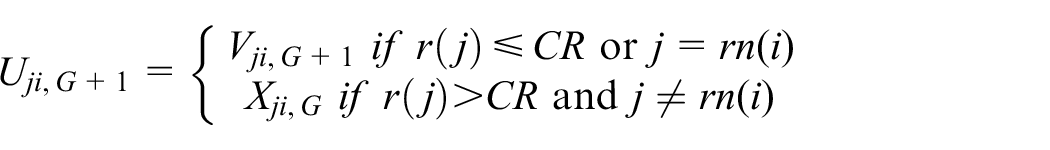
where j = 1, 2,…, d, and r(j) denotes the jth random number whose value lies between 0 to 1; CR, the crossover probability, controls the fraction of parameter values that are copied from the mutant vector. A randomly chosen index rn(i), where rn(i) ∈ {1, 2,…, D} to ensure that U_i,G+1 receives at least one parameter from V_i,G+1. ³⁶

• Step 4: Selection

This step aims at choosing the best solutions regarding the cost. Here, we choose either trail vector or target vector after calculating the fitness value for each chromosome. The following equation is used in the selection operation

$$X_{i,G+1}=\{\begin{array}{c}{U}_{i,G+1}\dots \mathrm{if}h(U_{i,G+1})\le h(X_{i,G})\hfill \\ \multicolumn{1}{c}{X_{i,G}\dots \mathrm{Otherwise}}\end{array}$$

(13)

where, h represents the objective function to be minimized.

The results we obtained are used to test the best mutation, which has the highest value of both TP and TN, and thus, differential evolutionary algorithm contributes to choose the least number of genes or feature to be relied upon in the identification of epilepsy.^34,35

The operators of mutation and crossover: We use an improved DE method that is proposed by Baig et al. ³⁷ This improved model is developed using a float optimizer. In the beginning, they generated three random solutions among all available solutions; we consider each of the features extracted based on seven statistical equations that are mentioned above. Then the operator’s mutation and crossover are used between solutions, in which the operators were assigned in same manner as by Phung et al., ³⁸ crossover probability = 0.5 and amplification factor F = 1.

Thus, the results of applying the statistical functions are 2184 features for each signal, in addition to class name (normal/seizure) with a total number of 2184 of features. Given that we have 2184 as a total number of features, we select only the best 250 features among them. This number was determined based on many empirical experiments as shown by Figure 5.

Figure 5.

Number of features.

Depending on these features, we can classify signals automatically. Initial results proved that the proposed model is accepted and applicable to several databases.

The machine learning is widely used in various fields of classification and identification. ³⁹ It includes many types such as supervised learning, unsupervised learning, and semi-supervised learning. In this article, we used supervised learning to classify cases of epilepsy based on brain signals (EEG). For this reason, features extracted in previous step were used in two parts: training and testing. Thus, we used six commonly used classifiers which are Naïve Bayesian (NB), Decision Tree (DT), ANN, KNN, RF, and SVMs. Figure 6 shows this step.

Figure 6.

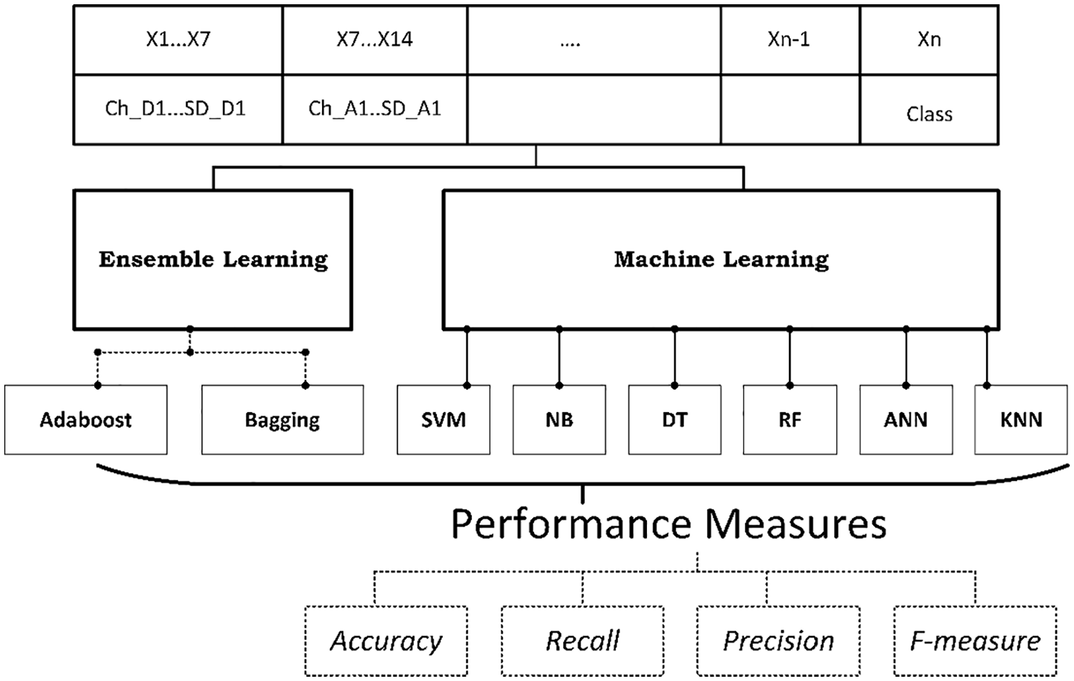
EEG classification step.

In general, there is a great deal between the ANN classifier and brain in humans. This method, ANN, is characterized by its powerful computing capability as well as its impact on data mining. Its vast learning and learning capacity cannot be ignored in training or learning, where ANN input layer can be considered as input to produce satisfactory results in terms of responsiveness. ⁴⁰ Back propagation (BP) is a method that is specifically used in the field of applying weight for a MLP. The key to this algorithm is based on principle of calculating partial derivatives, so that, they can almost find a function obtained from network, taking every neuron of weight vector into account. Nonlinear data can be categorized based on nonlinear activation functions in an easy and accessible manner.

In the field of epileptic seizures identification, it is possible to rely on these techniques, MLP structure with the BP algorithm, as they are considered suitable methods in the field of classification. For WT coefficients, the quantity of neurons in the input layer is equal to the number of features chosen by DE.^41,42 In this way, 15 unseen layer neurons are selected, each containing two output layers, which is later classified as an infected or normal case.

SVM: It is one of the most famous techniques in machine learning, used in classification, and related to state-of-the-art algorithms. ⁴¹ The margin calculation is main idea of this technique. It separates the classes by placing these margins, which are placed in a deliberate manner, as they should distance the classes from the maximum distance, thus reducing the errors in the classification process. ⁴³

Naive Bayes: is one of the simple classifiers that is based on principle using assumptions of independence Bayes statistic. ⁴⁴ One of these assumptions is that the presence of a feature or lack of it, which does not affect any other feature in terms of presence or absence of that feature. Thus, all features in the class have their own independent role in probability. This is a good value for small training data, which is capable of estimating differences in the variables necessary in classification process. In our research, cross-validation is used to classify epilepsy by input to minimize the effect of zero probability.

DT: It is one of the methods that are used to expect response depending on instance space and its recursive partition. This method is characterized by its rules, as these rules act as a catalyst to catch the final node. This method is named by this because of the similarity between tree structure and nodes number. Each node contains two options in most cases, either a decision node or a leaf node. It starts from the bottom, the root, up to the top, the node, which is the part that reaches the category where the data are sorted. In this research, we will adopt this type of classification, starting with binary splits, which will be subject to the best standard in the process of examination.

We will also rely on a C4.5 DT, distributed in 1993 by Ross Quinlan. ²⁶ This method has the power and speed to express data structures, in addition to be a somewhat traditional method, and the diversity of options has positive impact on classification process and quality of its results.

KNN is considered as one of the efficient classifiers in terms of time complexity, simplicity, and commonly used. ³⁷ The KNN method is based on calculating the degree of similarity between all the vectors in the training and testing packages, and then, retrying the test to same class of vectors, which attains highest similarity. Typically, the k value is determined to be odd in KNN, where odd value is used to avoid neutralization, for example 1, 3, and 5. In our study, k is equal to 1.

Ensemble learning is a process in which more than one classifier such as NB, DT, neural network, and others are gathered to get a new type. This field, ensemble learning, has been a crucial subject in science since the 1990s. As noted by the interested in this field, when the collection of more than one learner and its characteristics are obtained better performance compared to the implementation of one classifier. ⁴⁵ In some cases, when the database size is huge, it is, not possible to upload it to the memory in one stage; therefore, another method is used to upload the database incrementally. In addition, the capacity of a classifier to go up against new data and classes by advancing the classifier without its being completely retrained is known as incremental learning. Incremental learning has been effectively connected to numerous order issues, where the information is changing and is not all accessible without a moment’s delay. ⁴⁶ Incremental learning techniques should satisfy some conditions such as the ability to use new data for advanced learning, Moreover, it should train the classifier without the need to access original data, and it should benefit from previously acquired knowledge. Here are two types of Ensemble learning methods:

One of the most famous methods in ensemble learning is a combination of weak classifiers with each other to get out a new better one and is usually used to reduce the level of variance and bias and to distinguish between the weak and strong classifiers. The weak learner is weak in terms of the link to the real classification, while the strong learners are a very strong link to the real classification. ²⁰

Bagging is another type of methods used in ensemble learning, also called bootstrap aggregating. This type is specifically used to increase the accuracy and stability of machine learning classifiers. It can also reduce the contrast ratio in addition to its ability to deal with over fitting. ²² It should be noted that this type can be worked on in the categories of classification and regression. Summarization of our proposed method is showed in Figure 7.

Figure 7.

Proposed method.

Data sets description

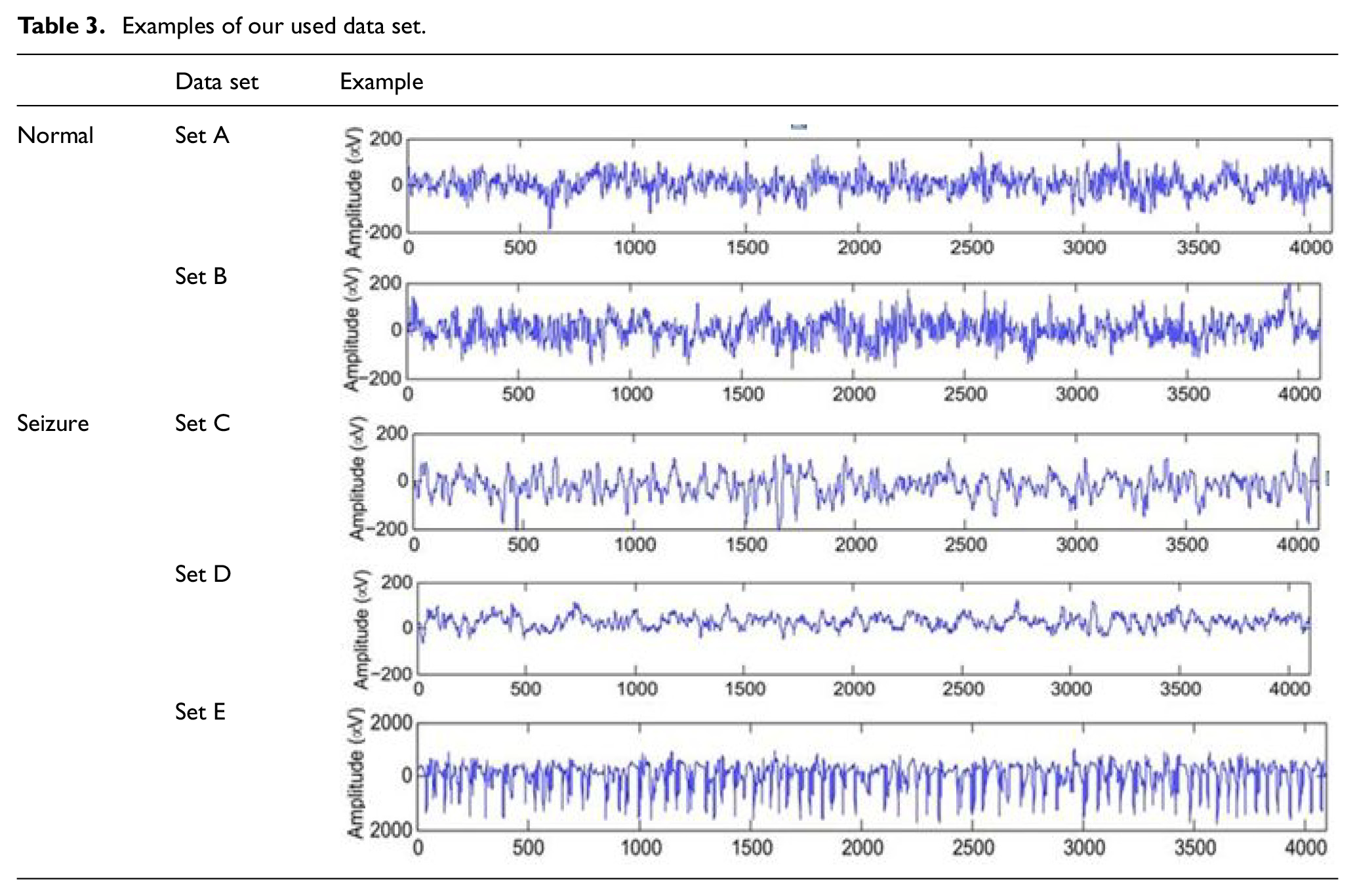
Epilepsy data collected by the Department of Epilepsy at the University of Bonn, Germany, are easily available for free to the public (Table 2). This database is composed of five different sections of EEG signals, and these sections are represented by symbols from A to E. Each of these sections consists of 100 signals, where recording time was about 23.6 s. In order to record the data with the most accurate way, they used an amplified system with 128 signal channels, which the output resulted in a 173.61 Hz of the sampling rate and a bit depth of 12-bit resolution, calculating it by the octave of 0.53–40 bandwidth. Taking into consideration, applying a band-pass filter (12 dB/Oct).

Table 2.

Examples of database in normal and seizure cases.

Set name	Annotation of data	Size	Acquisition circumstances
Set A	Z000.txt—Z100.txt	564 kB	Five healthy subjects with opened eyes
Set B	O000.txt—O100.txt	611 kB	Five healthy subjects with closed eyes
Set C	N000.txt—N100.txt	560 kB	Five epileptics with seizure free status
Set D	F000.txt—F100.txt	569 kB	Five epileptics with seizure-free status, inside five epileptogenic zone
Set E	S000.txt—S100.txt	747 kB	Five subjects during seizure activity

Sections A and B were collected from healthy volunteers, who did not suffer from epilepsy, such that section A was recorded when volunteers’ eyes were open, while in Section B, signals collected when their eyes were closed (Table 3). In sections C, D, and E, signals were recorded for individuals with epilepsy, In sections C and D; the signals were picked up from epileptic patients, but not during an occurrence of epilepsy, while the last Section E was taken from patients during an occurrence of epilepsy. ⁴⁷

Table 3.

Examples of our used data set.

	Data set	Example
Normal	Set A
	Set B
Seizure	Set C
	Set D
	Set E

Results and discussion

All experiments are based on the common 10-fold cross-validation, in which data are divided into 10 parts randomly equally. Each of these parts, which is called the subset, is used for training purposes, except for one set used for testing purposes. This is a recurrent process for 10 times and is called fold. Each subset is used for testing purposes only once. In this case, we are sure that all instances in the feature’s matrix are applied in testing and training phase. The results, after repeated 10 times, are used to take the rate to perform one classification.

In our research, we imply recording in the EEG for evaluation purposes. The length of piece is a basic source that provides multiple EEG samples, which have been extracted from each subject. Since this process, 10-fold cross-validation, is repeated 10 times, we get different results.

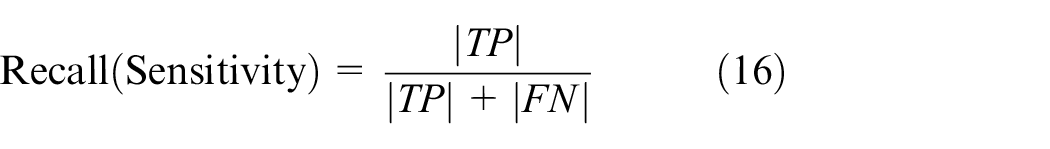
To evaluate our model, we use accuracy, recall, precision, and F-Measure, see formula below: there are many commonly used metrics for evaluating the performance of any systems. In this article, we will use four of them. The earlier confusion matrices are used to derive the four performance measures adopted in this article according to the following equations

$$\mathrm{Accuracy}:=\frac{\left|\mathrm{TN}\right|+\left|\mathrm{TP}\right|}{\left|\mathrm{TN}\right|+\left|\mathrm{TP}\right|+\left|\mathrm{FN}\right|+\left|\mathrm{FP}\right|}*\left(100\right)$$

(14)

$$\mathrm{Precision}:=\frac{\left|\mathrm{TP}\right|}{\left|\mathrm{TP}\right|+\left|\mathrm{FP}\right|}$$

(15)

$$\mathrm{Recall}\left(\mathrm{Sensitivity}\right)=\frac{\left|\mathrm{TP}\right|}{\left|\mathrm{TP}\right|+\left|\mathrm{FN}\right|}$$

(16)

$$\mathrm{F}-\mathrm{Measure}=2\times \frac{\mathrm{Precision}\times \mathrm{Recall}}{\mathrm{Precision}+\mathrm{Recall}}$$

(17)

Regarding signals processing, it is often found to have the tendency to favor a certain feature set on another set for reaching a specific goal in addition to have a dependent application and a dependent representation. This work relies on the application of different algorithms of supervised machine learning, in addition to the use of different measures to evaluate the performance and efficiency of differential evolutionary. This section is specifically concerned with how these measures are performed in different types and in different situations.

This part of the study presents results of some experiments related to evaluating the performance of proposed approach. It also includes a study about the effect of using different methods of distance used in this approach and deciding the accuracy of classification. Tables 4–12 display the experimental results. Where these tables presented accuracies of classification based on 10-fold cross-validation technique. In Tables 4–9, six different types of classifiers were used to get the classification accuracy, including ANN, SVM, NB, RF, DT, and KNN. In Tables 11 and 12, the accuracy of classification was obtained using the Bagging and AdaBoost methods in ensemble learning. Table 4 displays the evaluation results for the SVM technique. Based on some experiments, it was noted that there was a major difference in the results of these experiments, which were repeated in 16 different cases of data sets.

Table 4.

Results of proposed model with SVM.

	Case	Accuracy	Recall	Precision	F-measure
SVM	A-C	100	1.000	1.000	1.000
	A-D	99	0.990	0.990	0.990
	A-E	100	1.000	1.000	1.000
	B-C	99	0.980	1.000	0.990
	B-D	99.5	0.990	1.000	0.995
	B-E	100	1.000	1.000	1.000
	A-CD	99.33	0.990	1.000	0.995
	A-DE	98.33	0.980	0.995	0.987
	B-CD	98.33	0.975	1.000	0.987
	B-DE	98.33	0.975	1.000	0.987
	AB-C	99	0.980	0.990	0.985
	AB-D	99	0.980	0.990	0.985
	AB-E	99.66	0.990	1.000	0.995
	AB-CD	98.5	0.975	0.995	0.985
	AB-DE	98	0.970	0.990	0.980
	AB-CDE	97.6	0.967	0.993	0.980

SVM: support vector machine.

Table 5.

Results of the proposed model with Decision Tree.

	Case	Accuracy	Recall	Precision	F-measure
DT	A-C	96	1.000	0.926	0.962
	A-D	94	0.940	0.940	0.940
	A-E	99.5	1.000	0.990	0.995
	B-C	98.5	0.980	0.990	0.985
	B-D	98.5	0.990	0.980	0.985
	B-E	99.5	1.000	0.990	0.995
	A-CD	97.33	0.985	0.975	0.980
	A-DE	97.66	0.985	0.980	0.983
	B-CD	99	0.995	0.990	0.993
	B-DE	98.66	1.000	0.980	0.990
	AB-C	96	0.940	0.940	0.940
	AB-D	97.66	0.980	0.951	0.966
	AB-E	99.66	1.000	0.990	0.995
	AB-CD	96.25	0.950	0.974	0.962
	AB-DE	97.5	0.980	0.970	0.975
	AB-CDE	97.6	0.987	0.974	0.980

DT: decision tree.

Table 6.

Results of the proposed model with random forest.

	Case	Accuracy	Recall	Precision	F-measure
RF	A-C	98.5	1.000	0.971	0.985
	A-D	97	0.970	0.970	0.970
	A-E	100	1.000	1.000	1.000
	B-C	99	0.980	1.000	0.990
	B-D	99	1.000	0.980	0.990
	B-E	100	1.000	1.000	1.000
	A-CD	98.66	0.995	0.985	0.990
	A-DE	99.33	0.995	0.995	0.995
	B-CD	99	0.990	0.995	0.992
	B-DE	99.33	0.995	0.995	0.995
	AB-C	98.66	0.970	0.990	0.980
	AB-D	98.33	0.980	0.970	0.975
	AB-E	100	1.000	1.000	1.000
	AB-CD	98.5	0.980	0.990	0.985
	AB-DE	99	0.995	0.985	0.990
	AB-CDE	98.4	0.983	0.990	0.987

RF: random forest.

Table 7.

Results of the proposed model with ANN.

	Case	Accuracy	Recall	Precision	F-measure
ANN	A-C	100	1.000	1.000	1.000
	A-D	99	0.980	1.000	0.990
	A-E	99	0.980	1.000	0.990
	B-C	99	1.000	0.980	0.990
	B-D	99	1.000	0.980	0.990
	B-E	100	1.000	1.000	1.000
	A-CD	99.33	0.980	0.990	0.985
	A-DE	99	1.000	0.971	0.985
	B-CD	99	1.000	0.980	0.990
	B-DE	97.3	0.990	0.934	0.961
	AB-C	100	1.000	1.000	1.000
	AB-D	97.6	0.995	0.971	0.983
	AB-E	99.3	1.000	0.990	0.995
	AB-CD	98	0.985	0.975	0.980
	AB-DE	97	0.975	0.970	0.973
	AB-CDE	97.4	0.980	0.956	0.968

ANN: artificial neural network.

Table 8.

Results of the proposed model with k-nearest neighbor.

	Case	Accuracy	Recall	Precision	F-measure
KNN	A-C	99.5	1.000	0.990	0.995
	A-D	99.5	1.000	0.990	0.995
	A-E	100	1.000	1.000	1.000
	B-C	98	0.960	1.000	0.980
	B-D	99	0.980	1.000	0.990
	B-E	100	1.000	1.000	1.000
	A-CD	98	0.975	0.995	0.985
	A-DE	98.66	0.985	0.995	0.980
	B-CD	97	0.945	0.970	0.962
	B-DE	97.66	0.970	0.995	0.982
	AB-C	97	0.940	0.975	0.950
	AB-D	98.66	0.970	0.990	0.980
	AB-E	99.66	0.990	1.000	0.995
	AB-CD	96.75	0.945	0.989	0.967
	AB-DE	97.5	0.975	0.974	0.974
	AB-CDE	97	0.957	0.993	0.974

KNN: k-nearest neighbor.

Table 9.

Results of the proposed model with Naïve Bayes.

	Case	Accuracy	Recall	Precision	F-measure
NB	A-C	98.5	0.980	0.990	0.985
	A-D	90.5	0.870	0.935	0.902
	A-E	100	1.000	1.000	1.000
	B-C	98.5	1.000	0.971	0.985
	B-D	97	95.000	0.990	0.969
	B-E	100	1.000	1.000	1.000
	A-CD	96.6	0.970	0.933	0.951
	A-DE	83.330	1.000	0.667	0.800
	B-CD	98.3	1.000	0.952	0.976
	B-DE	86.33	0.990	0.712	0.828
	AB-C	98.66	0.995	0.985	0.990
	AB-D	89.33	0.850	0.988	0.914
	AB-E	100	1.000	1.000	1.000
	AB-CD	98.25	0.985	0.980	0.983
	AB-DE	86.75	0.995	0.794	0.883
	AB-CDE	0.956	1.000	0.901	0.948

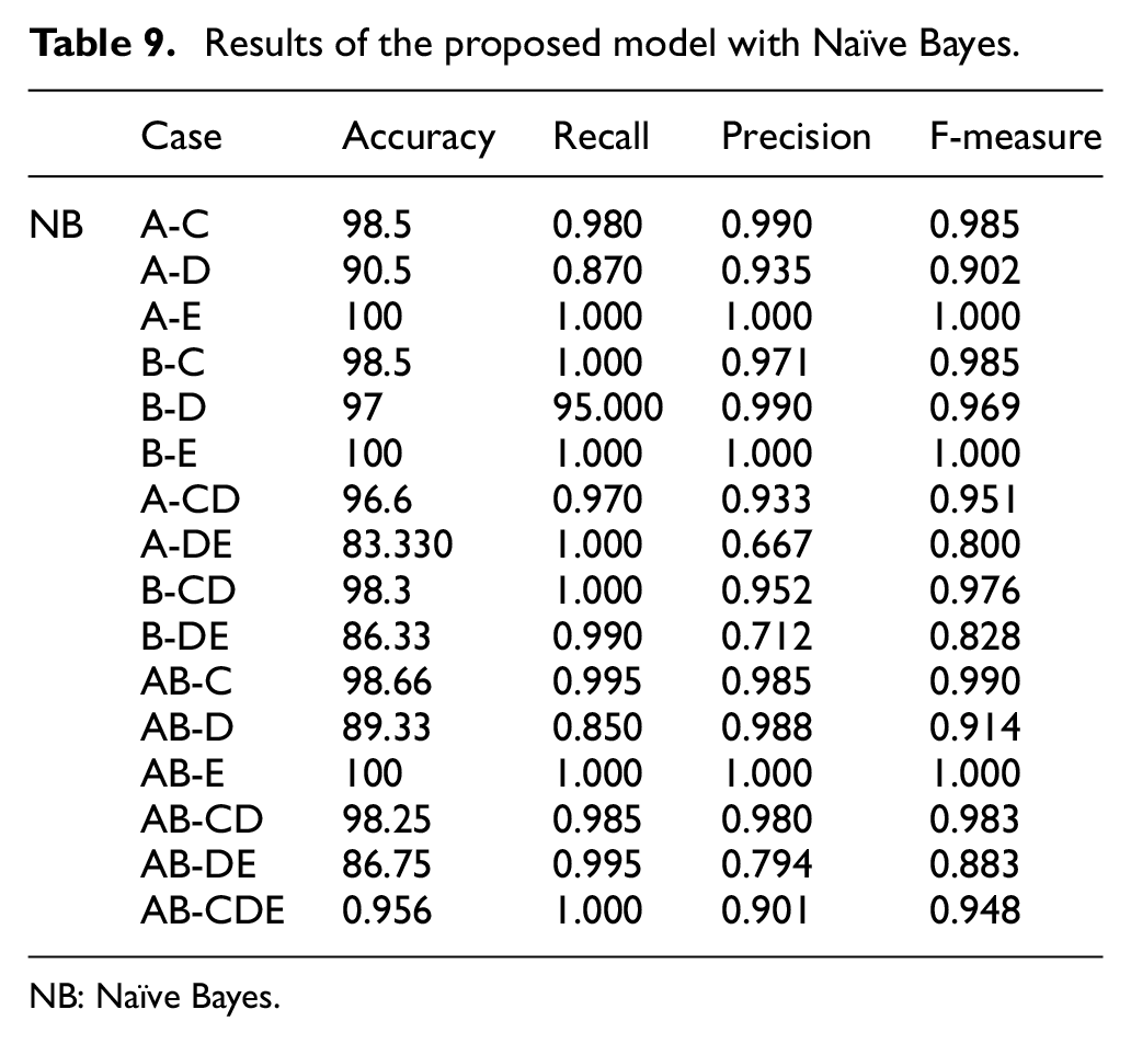
NB: Naïve Bayes.

Table 10.

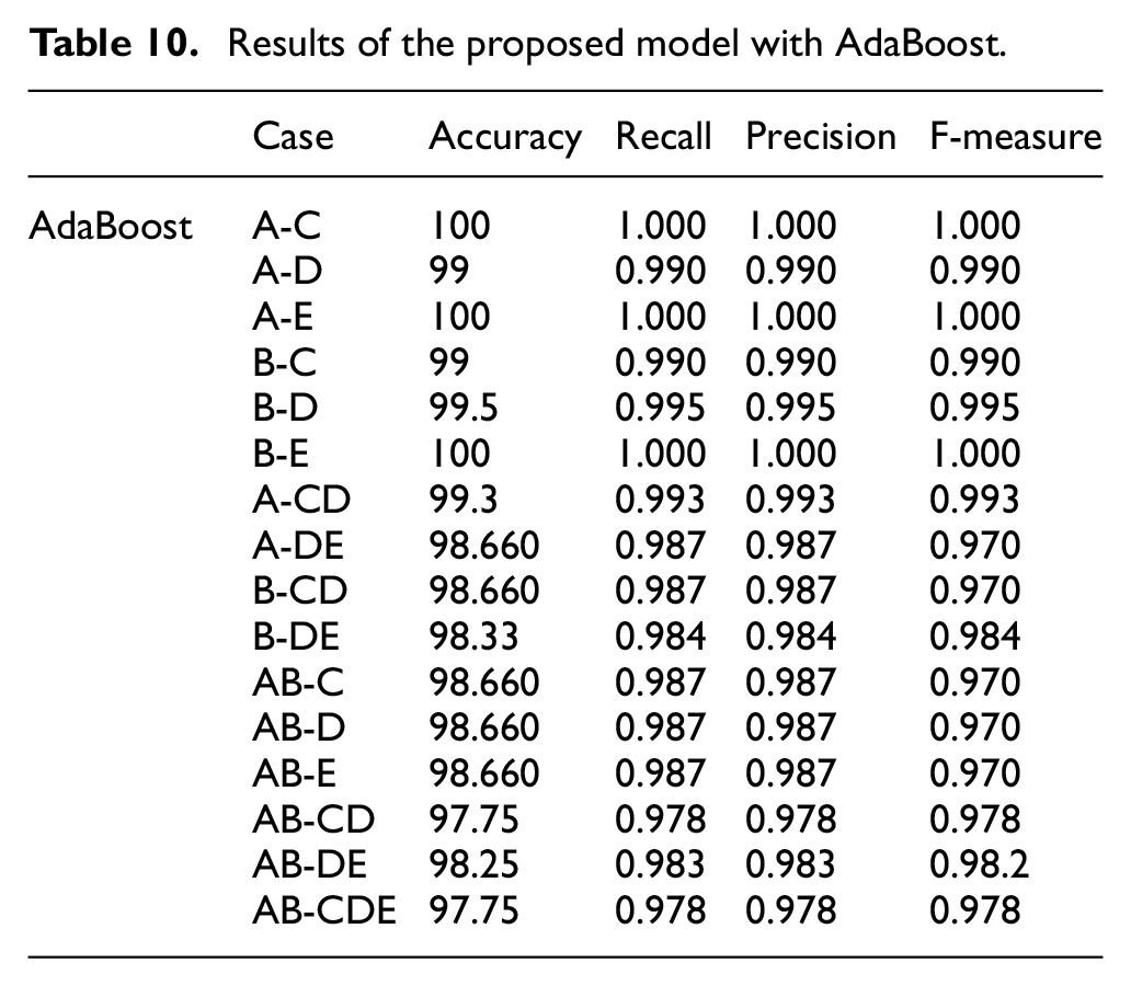
Results of the proposed model with AdaBoost.

	Case	Accuracy	Recall	Precision	F-measure
AdaBoost	A-C	100	1.000	1.000	1.000
	A-D	99	0.990	0.990	0.990
	A-E	100	1.000	1.000	1.000
	B-C	99	0.990	0.990	0.990
	B-D	99.5	0.995	0.995	0.995
	B-E	100	1.000	1.000	1.000
	A-CD	99.3	0.993	0.993	0.993
	A-DE	98.660	0.987	0.987	0.970
	B-CD	98.660	0.987	0.987	0.970
	B-DE	98.33	0.984	0.984	0.984
	AB-C	98.660	0.987	0.987	0.970
	AB-D	98.660	0.987	0.987	0.970
	AB-E	98.660	0.987	0.987	0.970
	AB-CD	97.75	0.978	0.978	0.978
	AB-DE	98.25	0.983	0.983	0.98.2
	AB-CDE	97.75	0.978	0.978	0.978

Table 11.

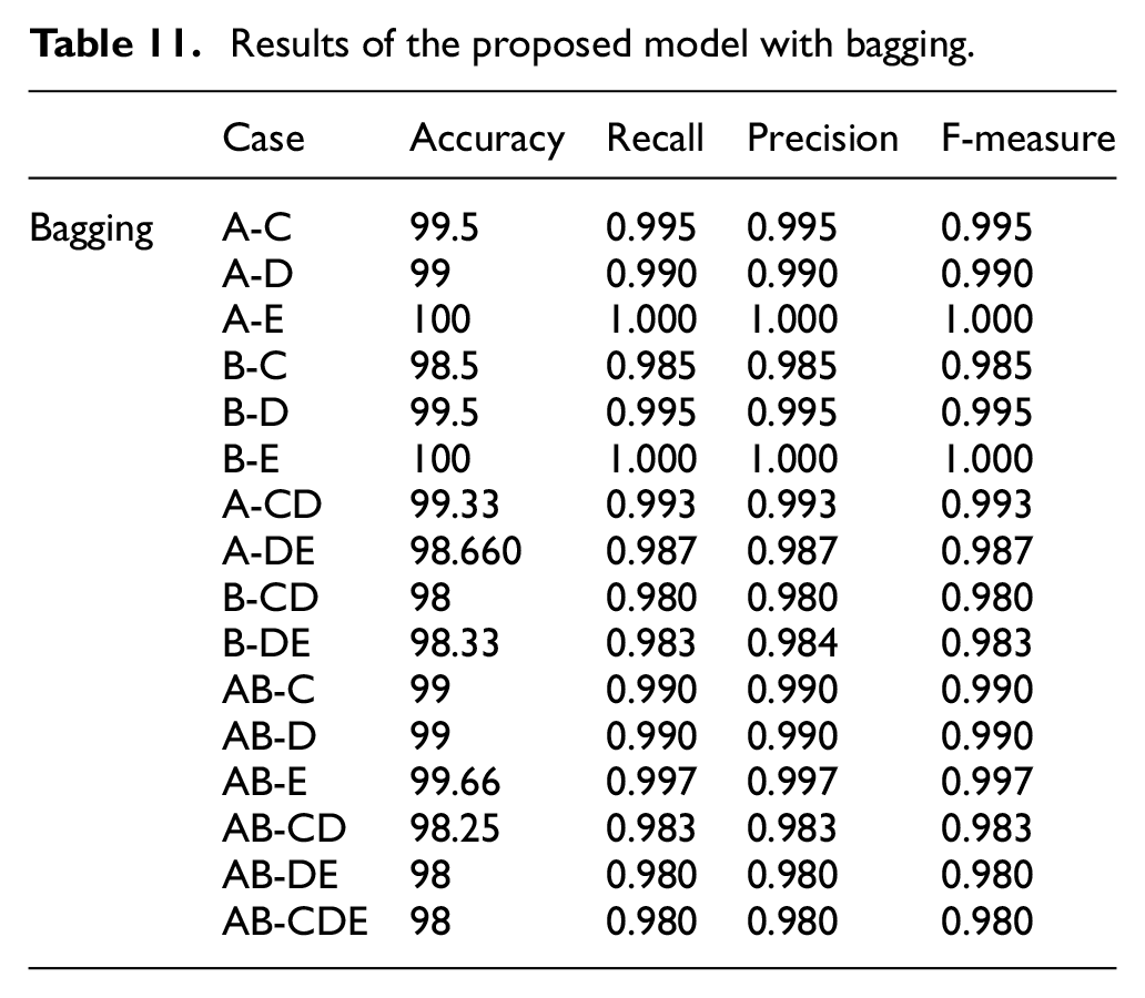
Results of the proposed model with bagging.

	Case	Accuracy	Recall	Precision	F-measure
Bagging	A-C	99.5	0.995	0.995	0.995
	A-D	99	0.990	0.990	0.990
	A-E	100	1.000	1.000	1.000
	B-C	98.5	0.985	0.985	0.985
	B-D	99.5	0.995	0.995	0.995
	B-E	100	1.000	1.000	1.000
	A-CD	99.33	0.993	0.993	0.993
	A-DE	98.660	0.987	0.987	0.987
	B-CD	98	0.980	0.980	0.980
	B-DE	98.33	0.983	0.984	0.983
	AB-C	99	0.990	0.990	0.990
	AB-D	99	0.990	0.990	0.990
	AB-E	99.66	0.997	0.997	0.997
	AB-CD	98.25	0.983	0.983	0.983
	AB-DE	98	0.980	0.980	0.980
	AB-CDE	98	0.980	0.980	0.980

Table 12.

Summary of t-test between any two of the compared machine learning classifiers.

	SVM	DT	RF	ANN	KNN	NB	AdaBoost
SVM
DT	0.003148
RF	0.404288	6.066E-05
ANN	0.097006	0.0206186	0.2757108
KNN	0.002118	6.066E-05	0.0420721	0.096780617
NB	0.055294	0.0827592	0.0581649	0.058974827	0.066557881
AdaBoost	0.175023	0.0046666	0.4418827	0.216373444	0.006757366	0.057405
Bagging	0.199037	0.0035847	0.4976326	0.175746213	0.002395243	0.057175	0.371053

SVM: support vector machine; DT: decision tree; RF: random forest; ANN: artificial neural network; KNN: k-nearest neighbor; NB: Naïve Bayes.

P-values of the t-test are given, and significant p-values at 90% confidence level are bold faced.

From Table 4, we note that all cases achieved 100% of precision, except AB-CD, AB-DE, AB-CDE, AB-C, AB-D, A-DE, and A-D which achieved about 0.99. We note the decline in the level of accuracy in the samples consisting of a combination of AB together or when we compare the data of the case D.

As for the recall, accuracy, and F-measure results, A-C, A-E, and B-E sets achieved 100%. For the rest of the sets, the results ranged from 0.967 to 0.99 for recall and 97.6 to 99.66 for accuracy, while the F-measure results ranged from 0.980 to 0.995.

Based on these results, we can conclude that this classifier can achieve high results, making it a suitable option in the diagnosis of epileptic seizures cases, regardless of the different status of the patient, whether closed-eye or open-eye, infected spasticity or if the person is healthy and non-infected.

The results of Table 5 represent the measurement of the DT performance with the proposed model. Where the accuracy, recall, F-measure, and precision measurements are all decreased when compared to the previous classifier. However, some results were recorded at 100% recall with some sets, specifically, at some intersections with case E, as in AE, BE, B-DE, and AB-E sets. A result of 100% was also shown in the A-C set. For accuracy, precision, and F-measure, the results were approximately 99% in AB-E, B-CD, B-E, and A-E sets, with the lowest values in the A-D set at 94%.

The results of Table 6 represent the performance measures of the RF classifier. Results show that the values of the four performance measures were 100% in the AE, BE, and AB-E sets, and the results were 100% in AC and BD with recall and BC with Precision. While the worst results were in A-D set of 97 with all the evaluation measures. So far, this is the same as the results of previous classifier but with an overview that is more suitable for use than DT. It achieved more efficient results for all sets.

Table 7 presents the results of the performance of the ANN Classifier, where the results were as follows: both A-C and B-E sets achieved 100% with all performance measures used. This result was also particularly significant for the A-D and A-E sets, as well as for the recall with five other sets, B-D, A-DE, B-CD, and AB-E B-C. The worst ratios were 97, 0.975, 0.934, and 0.973 for the measures, accuracy, recall, precision, and F-measure, respectively.

Tables 8 and 9 show the results of the proposed model performance analysis with the KNN and NB classifiers, respectively. They show the relative similarity between the values of performance measures, which is represented as follows: the four measures achieved high accuracy results of 100% with the A-E and B-E sets.

The KNN classifier achieved 100% for the A-C and A-D sets for recall. The same percentage of the B-D, AB-E, and B-C sets was achieved in terms of recall; the lowest values were shown in the AB-C set at the four measures. NB classifier achieved a precision of 100% in recall with B-C, A-DE, B-CD, and AB-CDE sets. But the results are significantly reduced compared to the other five, where the accuracy achieved 83.330 in the A-DE set and 0.667 for the same set with Precision. The 0.850 ratio of the recall is also in AB-D set.

Figure 8 below compares between the six machine learning classifiers regarding accuracy. The figure proved that the use of ANN is more efficient than other machine learning algorithms and this is proved by our work results where the accuracy reached 100%.

Figure 8.

Performance comparison of different machine learning techniques.

In Tables 10 and 11, the ensemble learning method was adopted to determine the accuracy of the classification process, and the quality and effect of the weight classifier were studied against other classifiers. Given the results in the tables, there is a little variation in the accuracy of the classification in line with the variation of types of ensemble learning that were used in the combination of classifiers. The results also show that the accuracy in the classification which was obtained from the Bagging method and the AdaBoost method were fairly compatible. Table 10 represents the results of AdaBoost and shows that the results ranged from 0.97% to 100% on the four measures adopted for evaluating the system. So that the sets A-C, A-E, and B-E achieved 100% at the four measures, while the AB-CDE and AB-CD sets had the lowest results of 0.79 for all measurements.

Similarly, the previous ensemble learning achieved fairly similar results for Bagging, ranging from 0.98% to 100%. The 100% result for A-E and B-E groups was confirmed.

Statistical analysis

In this study, we presented multi-DWT features-extraction model to classify cases of epilepsy by brain signals. In order to show the effectiveness of proposed model, we compared our best results that are achieved by applying SVM multi-DWT features-extraction model with results obtained by applying SVM DWT on data with full features (Tables 4 and 12, respectively).

Based on the results demonstrated in the above results, we have the following conclusions: with the used data sets, all classifier methods on average perform better than NB and DT. To determine whether the other classifier methods consistently outperform single classification methods, we also conducted the t-test. The results are shown in Table 12. Based on the t-test significant p-values at 90% confidence level, we have the following conclusions.

1. There is a significant difference between the SVM compared to ANN and SVM compared to KNN. This significant does not appear between SVM and RF, nor with AdaBoost and Bagging.

2. There is a significant difference between the KNN compared to AdaBoost and Bagging. Actually, KNN shows significant differences with all the other methods.

To determine whether the selected classifier methods consistently outperform single classification methods, we also conducted two-tailed Wilcoxon signed-rank test. Based on the test, we have the following conclusions:

1. There is a significant difference between the SVM compared to KNN. SVM is much better in this regards. However, T_crit = 13 for the SVM and ANN <17 (sum of rank), we cannot reject the null hypothesis (i.e. p ≥ .1), and so conclude there is no significant difference between SVM and ANN.

2. There are significant differences between KNN and AdaBoost and Bagging methods. Both methods outperform KNN based on the two-tailed Wilcoxon signed-rank test.

In general, we can conclude that the SVM has shown very promising results compared to other classification methods. In order to evaluate the significance of our proposed method, we performed Wilcoxon signed-rank test. This test calculates differences of pairs. The absolute differences are ranked after discarding pairs with the difference of zero. The ranks are sorted in ascending order. When several pairs have absolute differences that are equal to each other, each of these several pairs is assigned as the average of ranks that would have otherwise been assigned as shown in Table 13. The hypothesis is that the differences have the mean of zero. To show that this improvement is significant, we conducted Wilcoxon signed-rank test on differences between accuracies on data after applying DE on SVM multi-DWT extracted features and SVM DWT on data with full features. SVM is selected because it gets the highest improvements of accuracy in all cases with significance difference as shown before.

Table 13.

Average accuracy for all subsets on data with full features.

SVM DWT full features
A-C	A-D	A-E	B-C	B-D	B-E	A-CD	A-DE
98	96.5	99	98	97.33	100	96	97
B-CD	B-DE	AB-C	AB-D	AB-E	AB-CD	AB-DE	AB-CDE
96	96.33	98.66	95.5	98	96.25	96.66	96.5

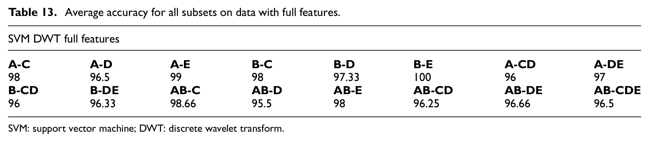
SVM: support vector machine; DWT: discrete wavelet transform.

Based on 95% confidence level, Table 14 shows that all cases except B-E improve the classification accuracy on the preprocessed data sets than the original data sets.

Table 14.

Summary of Wilcoxon signed-rank test between SVM DWT full features and multi-DWT features extraction.

	SVM DWT full features
SVM multi-DWT	A-C	A-D	A-E	B-C	B-D	B-E	A-CD	A-DE
	≤0.05	≤0.05	>0.05	≤0.05	≤0.05	>0.05	≤0.05	≤0.05
	B-CD	B-DE	AB-C	AB-D	AB-E	AB-CD	AB-DE	AB-CDE
	≤0.05	≤0.05	≤0.05	≤0.05	≤0.05	≤0.05	≤0.05	≤0.05

Conclusion

In this article, we presented a new model to detect seizure depending on EEG binary classification (normal/seizure). For this purpose, initially, we used multi-level DWT with different sub-bands to extract the features from raw data. Then, seven statistical functions were applied to the features. These functions include MAV, AVP, SD, variance, mean, skewness, and Shannon entropy. These function values were used as inputs to feed DE step in order to choose the strongest features. Finally, six supervised machine learning, three matching metrics, and two ensemble learning method were used to classify the signals. The results of this article proved to outperform proposed model.

In this article, we developed a method to classify cases of epilepsy by brain signals for high accuracy compared to related research. Here, we discuss the importance of features selection and features extraction to provide efficient results, as a preprocessing step before the classification process. Accordingly, DE and DWT were combined to obtain clear and effective results for the diagnosis of epilepsy. Thus, we have built a model that can perform an effective classification process. The problem of epileptic seizure is studied. Based on the high overall classification accuracy obtained, it is found that proposed hybrid algorithm can find a good subset of input features derived from wavelet coefficients of EEG signals. Using a combination of different WTs along with DE highly improved the classification power of the machine learning algorithm.

There are many differences in performance of supervised classifiers in terms of accuracy, precision, and recall measures. Through our experiments, we found that SVM were the best in terms of accuracy. Results also showed that the NB and KNN are convergent results. However, SVM has outperformed in EEG signals categorization. When applying F-measure on various data set cases and different classifiers, SVM gets the highest percentage of F-measure and Accuracy in all cases. As future work, we will apply our model to a larger EEG data set in the different application domain, and advanced DWT techniques can be considered for better results.