
Abstract
A Gauss process state-space model trained in a laboratory cannot accurately simulate a nonlinear system in a non-laboratory environment. To solve this problem, a novel Gauss process state-space model optimization algorithm is proposed by combining the expectation–maximization algorithm with the Gauss process Rauch–Tung–Striebel smoother algorithm, that is, the EM-GP-RTSS algorithm. First, a theoretical formulation of the Gauss process state-space model is proposed, which is not found in previous references. Second, a Gauss process state-space model optimization framework with the expectation–maximization algorithm is proposed. In the expectation–maximization algorithm, the unknown system state is considered as the lost data, and the maximization of measurement likelihood function is transformed into that of a conditional expectation function. Then, the Gauss process–assumed density filter algorithm and the Gauss process Rauch–Tung–Striebel smoother algorithm are proposed with the Gauss process state-space model defined in this article, in order to calculate the smoothed distribution in the conditional expectation function. Finally, the Monte Carlo numerical integral method is used to obtain the approximate expression of the conditional expectation function. The simulation results demonstrate that the Gauss process state-space model optimized by the EM-GP-RTSS can simulate the system in the non-laboratory environment better than the Gauss process state-space model trained in the laboratory, and can reach or exceed the estimation accuracy of the traditional state-space model.
Keywords
Introduction
In many engineering problems, there are a large number of complex nonlinear dynamic systems needed to estimate state with a time series of the sensor measurement. A nonlinear dynamic model should be established according to a nonlinear system, such as a nonlinear state-space model (SSM), consisting of a parametric state transition equation and measurement equation. The Gauss process (GP) model can be used to simulate the nonlinear state transition equation and the measurement equation separately. A non-parametric Gauss process state-space model (GPSSM) can be constructed, if we lack the knowledge of a nonlinear system to build a principled parametric model. For example, GPSSMs are used for target monitoring and location problems in wireless sensor networks.1,2
In order to train the GPSSM of a nonlinear system, its true system states are required. However, paradoxically, its states are usually unknown and needed to be estimated. At present, some methods and models are proposed to try to overcome training and estimating problems of the GPSSM.
Gauss process latent variable models (GPLVMs) 3 are first proposed to learn a system model with low-dimensional state-space and high-dimensional observation space. Later, GPLVMs are extended to the dynamic system to obtain GPBF-LEARN, which is a framework for learning GP-BayesFilters from weakly labeled training data only. 4 With specially tailored Particle Markov Chain Monte Carlo (MC) samplers, a fully Bayesian approach to inference and learning (i.e. state estimation and system identification) for GPSSMs is proposed by marginalizing state transition functions. 5 Although this method preserves a non-parametric representation of a system model, it requires that its measurement model should be known. Variational GPSSM is proposed by combining variational Bayes with sequential MC. 6 Through imposing a structured Gaussian variational posterior distribution over latent states, an inference mechanism for the GPSSM is proposed in order to address the nonlinear system identification. 7 Although the above works have been devoted to the GPSSM training based on the unknown true system states, unfortunately the problem has not been solved theoretically.
Thus, the best way to obtain an accurate GPSSM is still to have to acquire its true system states to train a state transition equation a measurement equation. In order to obtain true system states, it is necessary to build a state detection system with multiple types of sensors, which is expensive and not possible in some cases. When a homogeneous nonlinear system can be placed in a laboratory, such a state detection system can be constructed in the laboratory. After true states are obtained in the laboratory, a GPSSM of the homogeneous nonlinear system can be established.
However, our purpose is to simulate a nonlinear dynamic system in a practical application with GPSSMs, that is, the nonlinear dynamic system in a non-laboratory environment. Because noise and parameters in a non-laboratory environment differ from those of the homogeneous nonlinear system in a laboratory, simulating a homogeneous nonlinear system in a non-laboratory environment with a GPSSM trained in a laboratory could introduce a model bias, which will lead to an overfitting problem of state estimation.
In order to improve the accuracy of a GPSSM in a non-laboratory environment, a reasonable method is to eliminate its model bias by adaptively correcting the hyperparameters of the GPSSM that is trained in a laboratory.
Recently, parameter identification methods, combining the expectation–maximization (EM) algorithm 8 with smoothing algorithms, 9 are gradually recognized for parametric nonlinear SSMs. Given the input measurements and the output measurements, the EM estimates the parameters in a multivariable bilinear SSM as the robust and gradient-free computation of the maximum likelihood (ML) solution. 10 A parameter estimation method combining particle method with the EM is proposed to estimate the general SSM of nonlinear systems. 11 Recognizing the unknown noise covariance of a nonlinear system is studied through the EM and the moving horizon estimation. 12 The EM using the classical extended and ensemble versions of the Kalman smoother is proposed to estimate the model error covariance. 13 For nonlinear SSMs with multiplicative unknown parameters, an adaptive dispersion filter algorithm based on the EM is proposed. 14
Given training data, a GPSSM can be regarded as a special parametric SSM. Based on the maximum likelihood estimator/estimate (MLE) criterion, this article proposes a novel GPSSM optimization algorithm called as the EM-GP-RTSS, combining the EM algorithm with the Gauss process Rauch–Tung–Striebel smoother (GP-RTSS) algorithm, in order to improve the accuracy of GPSSMs simulating the nonlinear dynamic system in a non-laboratory environment.
First, a theoretical formulation of GPSSMs is proposed by expanding one-dimensional output prediction to a multidimensional output prediction in this article. This is an important work, but not seen in previous references. Second, the MLE criterion is used to describe the GPSSM optimization problem as the maximization of the measurement likelihood function. However, the analytical expression of the measurement likelihood function is difficult, and thus the EM is used to replace the difficult-to-maximize measurement likelihood function with the conditional expectation function (CEF). Third, a GPSSM optimization framework based on the EM is proposed in this article. The GP-RTSS algorithm is given to obtain the smoothed estimation distribution of the system state, which is required by the calculation of the CEF. Fourth, in order to calculate the integral of the CEF in the closed form, the MC numerical integral method is used to express an approximate CEF. Fifth, the variable metric method 14 is adopted for the optimization calculation of the approximate CEF. In the simulation experiment, a noise pendulum model is used as a representative of the nonlinear dynamic system to verify the effectiveness of the EM-GP-RTSS algorithm proposed in this article.
This article is organized as follows. In section “Background on GP,” we briefly review the background on GPs. In section “Optimization algorithm for GPSSM,” we describe the development of the GPSSM optimization algorithm in detail. In section “Simulation experiment,” the experimental results based on the noise pendulum model are presented to demonstrate the performance of the EM-GP-RTSS. Finally, the conclusion is drawn in section “Conclusion and future works.”
Background on GP
In this section, a standard GP model and a noise input prediction model are given. This section is the mathematical foundation for the development of the GPSSM optimization algorithm.
Standard GP model
A GP is a non-parametric tool for learning regression functions from the sample data. 15 Specifically, a GP represents a random process, whose outputs of sampling points obey to a joint Gaussian distribution. A GP can be fully described by its mean function and covariance function. Suppose there is a training data set from the following noise process

where

where

where

and whose variance is

where
Noise input prediction model
If the test input
The mean and variance of

where
Let

The variable
where

where
Optimization algorithm for GPSSM
In this section, the GPSSM optimization algorithm is developed with the EM and the GP-RTSS. The whole framework flowchart of the GPSSM optimization algorithm is shown in Figure 1. First, the training data are obtained to train an original GPSSM to simulate a nonlinear system in a laboratory. Second, the measurements of nonlinear dynamic systems are obtained in a non-laboratory environment. The EM is used to optimize the GPSSM of homogeneous system in the laboratory. Since calculating the CEF in the Expectation step (E-step) requires the smoothed distribution of system states, the GP-RTSS algorithm is introduced into the EM optimization framework. In the Maximization step (M-step), the CEF is maximized to obtain the iterative hyperparameters, which means to adjust the GPSSM at the same time. The E-step and the M-step are repeated alternately until convergence occurs, and the optimized GPSSM and the estimated states will be acquired at the end.

The flowchart of the GPSSM optimization.
GPSSM
This section gives a theoretical formulation of GPSSMs. The concept of GPSSMs is already proposed in Ko and Fox,4,16 and Deisenroth et al., 17 but a theoretical formulation of GPSSMs has not been found. Consider the traditional SSM of a discrete-time nonlinear system

where
The operating mechanism of the dynamic system is assumed to be constant, that is the corresponding SSM of the system is unchanged in a time window
The matrix

The set


where

The above formulas (12)–(16) define a formulated GPSSM, which can simulate the traditional nonlinear SSM described in formula (11).
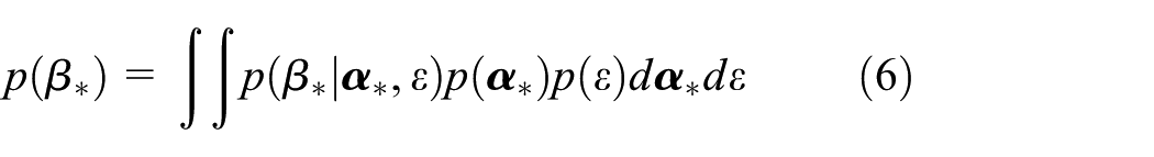
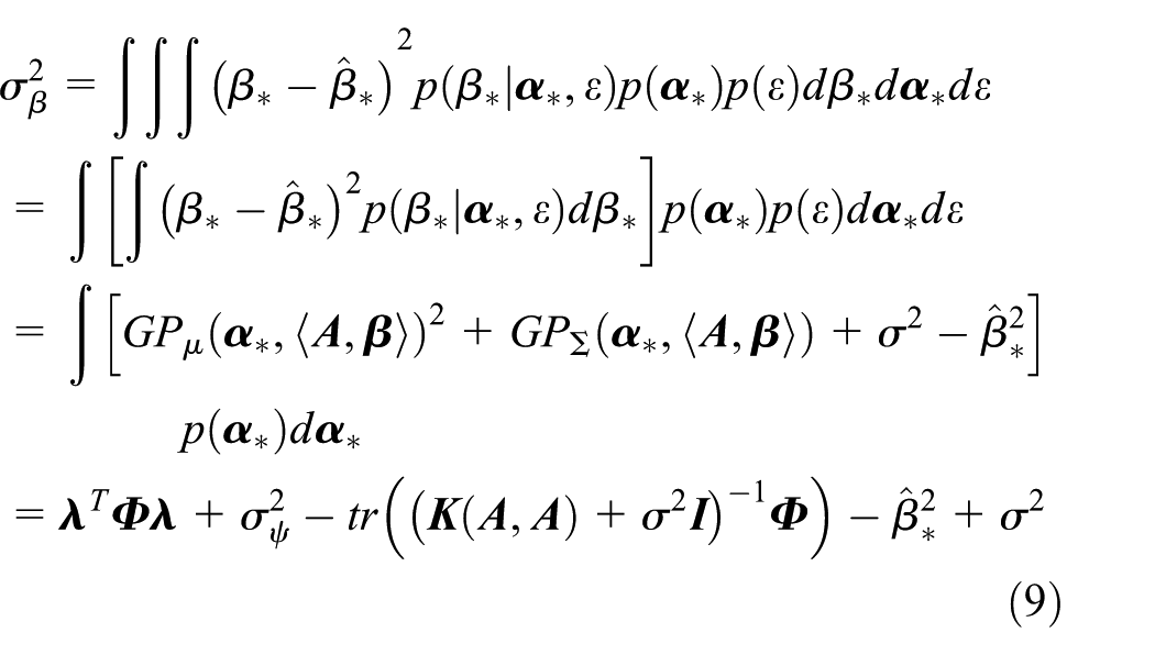
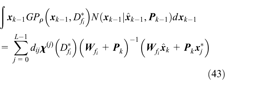
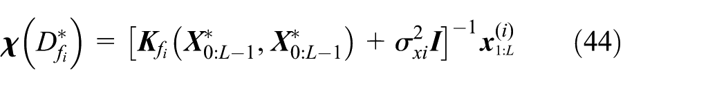
Because the system state is unknown, the state

If


where

Optimization algorithm framework
A GPSSM is theoretically expressed in the previous sections. In order to establish an instantiated GPSSM for a specific nonlinear system, the training data set of the state transition equation and the measurement equation should be given, that is, true states
An accepted method is to build a state detection system equipped with multiple types of sensors in a laboratory, by which true states can be measured to train a GPSSM. The GPSSM obtained in the laboratory is recorded as the GPSSM* in this article. The GPSSM* can obtain a satisfactory state estimation accuracy in a laboratory, but there is an overfitting problem of state estimation with the GPSSM* in a non-laboratory environment. This is because the environment of non-laboratory and laboratory are different, and then, the homogeneous nonlinear system is affected by several factors. Main differences are system noise, sensor noise, and system parameters. Then, the use of the GPSSM* in a non-laboratory environment would introduce a model bias. The lack of robustness is a drawback of the GPSSM*, but the GPSSM* simulates the basic mechanism of the homogeneous nonlinear system in the non-laboratory environment.
In order to solve this problem, the core idea of this article is to optimize the hyperparameters of the GPSSM* to obtain an approximate optimal model for a nonlinear system in a non-laboratory environment. Its state and measurement sequences obtained in a laboratory are denoted as

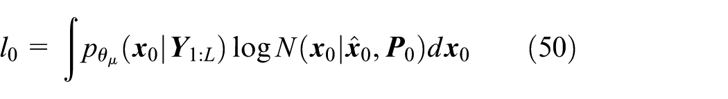
Because of the unknown

Given
The unknown system state sequence is denoted as

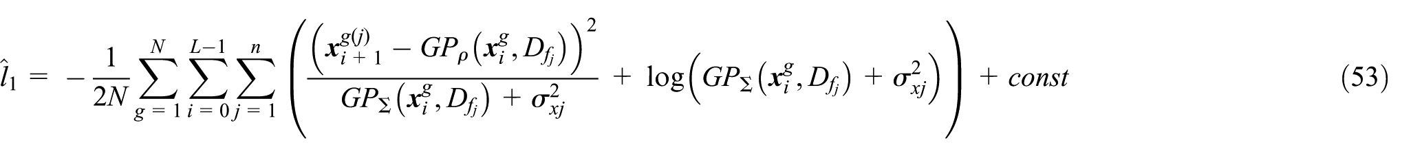
The hyperparameter
Let

Then

where
For
Step 1. Initialize
Step 2. Calculate
Step 3. Maximize
Step 4. Judge the convergence. If not,
In the next section, the GPSSM optimization algorithm is developed based on Framework 1.
Expectation step
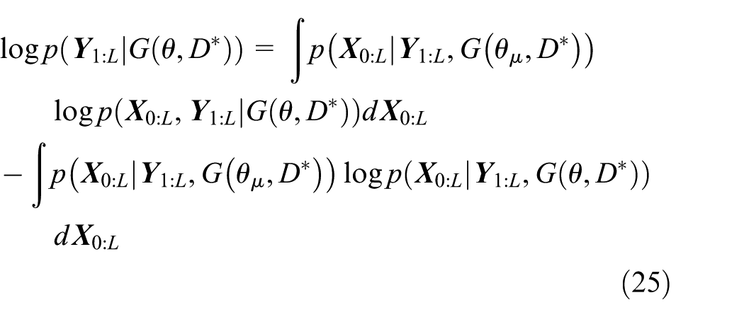
The first problem in Framework 1 is the specific expression of


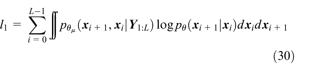

where
From formulas (29)–(31),
Filtering algorithm
For a nonlinear system state estimation problem, combining GPSSMs and Bayesian filtering algorithms, a variety of state estimation algorithms are proposed. Ko and Fox 16 present a unified framework including the extended Kalman filter (EKF), the unscented Kalman filter (UKF), and the particle filter (PF). And, Deisenroth et al. 17 propose the Gauss process–assumed density filter (GP-ADF) to acquire the state estimation mean and covariance matrix accurately.
Combining GP-BayesFilters with the Rauch–Tung–Striebel (RTS) smoother, the corresponding RTS smoothing algorithms can be obtained directly. These algorithms use the GP based on the noise-free test input, and the predicted covariance matrix is a diagonal matrix only, which cannot describe the correlation among the output data. Deisenroth et al. 19 propose an analytical RTS smoother called as GP-RTSS algorithm, which is able to predict based on the noise test input and is proved to be more robust. The GP-RTSS algorithm is obtained by combining the RTSS algorithm with the GP-ADF algorithm.
The filtered distribution of the system state


where
The filtered distribution of

In the step (4) of the above formula (35),

In step (1) of formula (36),
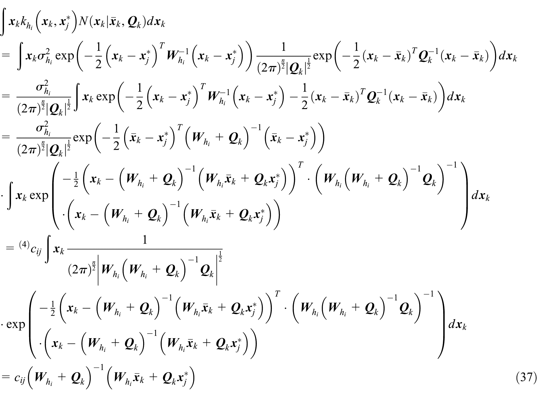

In step (3) of formula (37), the integral is the expectation operation on

Smoothing algorithm
Algorithm 1 accurately calculates the mean vector and the covariance matrix of the filtered estimation. Combining the GP-ADF with the RTS smoother, the distribution of the smoothed estimation can be calculated as follows


After executing Algorithm 1, the only unknown quantity is the matrix
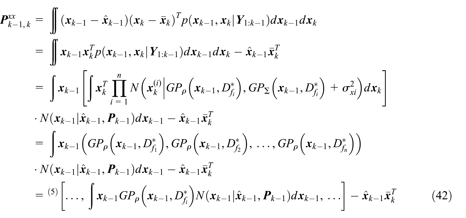
In step (5) of formula (42), the calculation of the integral term is similar to formula (36)

Thus, the GP-RTSS can be described as Algorithm 2.

Maximization step
Algorithm 2 can obtain the smoothed distribution of the GPSSM. Next, the joint smoothed distribution

where

Then

In step (3) of formula (48),

Thus,


The variables
Similarly, for

Based on the above content,
After
From the lemma of Deisenroth et al.,
19
when
Final optimization algorithm
The final optimization algorithm is described formally in this section. It is called as the EM-GP-RTSS algorithm, because it mainly consists of the EM algorithm and the GP-RTSS algorithm.
The key of Algorithm 3 is to replace the difficult-to-maximize measurement likelihood function with the CEF, as the MLE of hyperparameters for the expected GPSSM can be acquired asymptotically through iterative optimizing the CEF. Meanwhile, Algorithm 3 outputs the smoothed estimation at each EM iteration. Then, Algorithm 3 can also be called as a joint state estimation and model optimization algorithm for the GPSSM.

The computational complexity of Algorithm 3 depends on the two parts of the suboperation: the first is to compute the smoothed distribution; the second is to compute the approximate CEF. For the GPSSM described in this article, the computational complexity of GP-RTSS algorithm is
Simulation experiment
In this section, the computer simulation experiments are carried out to verify the performance of the EM-GP-RTSS algorithm. The noise pendulum system is selected as the simulated object by the GPSSM in these experiments. Because both its state transition equation and measurement equation are typical nonlinear forms, it is often used to verify the performance of the nonlinear filtering and smoothing algorithms.17,19
In this study, all experiments are performed using MATLAB R2013a on an Intel i5 quad-core 2.90-GHz 64-bit machine with 4 GB RAM.
Experimental settings
For a noise pendulum system with the unit length and the unit mass, its standard form of the discrete-time nonlinear SSM can be established as follows

where

where q is the spectral density.
On one hand, the nonlinear SSM (equation (55)) is served as a benchmark model to test the EM-GP-RTSS; on the other hand, it provides true states to train the GPSSM* that is taken as the GPSSM in the laboratory. We get different instantiated pendulum models (equation (55)) by setting different values for parameters
Parameter settings of five pendulum models.

Five pendulum models in Table 1 represent five homogeneous nonlinear dynamic systems. The pendulum model0 is used as the model in the laboratory that provides true states. The remaining four pendulum models describe noise pendulum systems in the different non-laboratory environments. For the pendulum models1–3, we set the different values of
By running the pendulum model0,

where
Experimental results
True states

The true states obtained by the pendulum model0.

The measurements obtained by the pendulum models0–4.
Hyperparameters of GPSSM*.

GPSSM: Gauss process state-space model.
Hyperparameters of GPSSM1–4.

GPSSM: Gauss process state-space model.
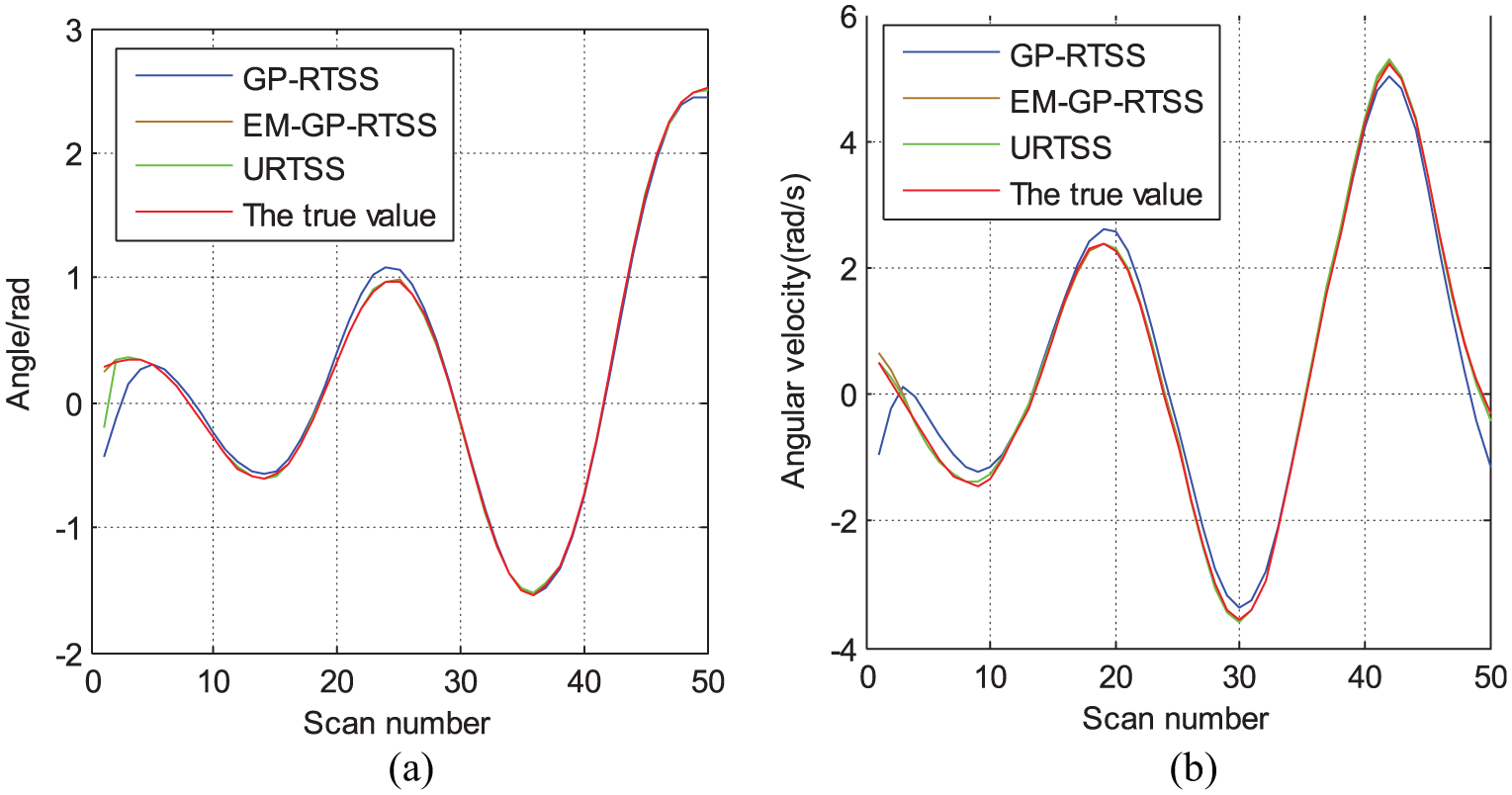
Figures 4–7 show the smoothed estimation mean of pendulum models1–4 obtained after running the EM-GP-RTSS to optimize the GPSSM*, respectively. And, the estimation of the GP-RTSS with the GPSSM* and the estimation of the URTSS with the true SSM (53) are also given. From Figures 4–7, it can be seen that the smoothed estimation mean of the EM-GP-RTSS can more accurately follow true states for the pendulum models1–4 than that of the GP-RTSS with the GPSSM*, which can also be seen from the corresponding standard deviation in Table 4. Therefore, it demonstrates that directly applying the GPSSM* to simulate these non-laboratory pendulum models1–4 introduces the model bias. It can be seen from Table 4 that the GP-RTSS with GPSSMs1–4 can reach or exceed the accuracy level of the URTSS with the SSMs1–4.

The smoothed estimation results for the pendulum model1: (a) angle smoothing estimation mean and (b) angular velocity smoothing estimate mean.

The smoothed estimation results for the pendulum model2: (a) angle smoothing estimation mean and (b) angular velocity smoothing estimate mean.

The smoothed estimation results for the pendulum model3: (a) angle smoothing estimation mean and (b) angular velocity smoothing estimate mean.
The smoothed estimation results for the pendulum model4: (a) angle smoothing estimation mean and (b) angular velocity smoothing estimate mean.
Standard deviation of smoothed estimation mean.

EM: expectation–maximization; GP: Gauss process; RTSS: Rauch–Tung–Striebel smoother; URTSS: unscented Rauch–Tung–Striebel smoother.
The one-step prediction performances of GPSSMs1–4 and the GPSSM* are tested in order to further discuss the advantage of GPSSMs1–4. Run pendulum models1–4 again in the time period
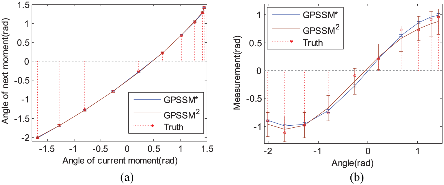
The prediction distributions from the GPSSMs1–4 are compared with the prediction distributions from the GPSSM*, as shown in Figures 8–11. The error bars show the twice standard deviations of the state prediction distributions or the measurement prediction distributions. The red circle indicates the corresponding true value of the prediction. The distributions obtained by the GPSSMs1–4 can contain the true values within the twice standard deviations. The true value appears in the range of the twice standard deviations of the distributions from the GPSSMs1–4 with the probability 95.5%. Except the pendulum model4, the prediction distributions of the GPSSM* cannot contain the true value in the twice standard deviations. When the noise of a nonlinear dynamic system increases in these non-laboratory environments, the confidence of the prediction distribution with the GPSSM* is lower than that with the GPSSMs1–4 optimized by the EM-GP-RTSS. And, the mean values of the predicted distributions with the GPSSMs1–4 are closer to the true value.

The one-step prediction distributions with GPSSM* and GPSSM1 for the pendulum model1. (a) The prediction distribution of the state transition equation GP model. (b) The prediction distribution of the measurement equation GP model.
The one-step prediction distributions with GPSSM* and GPSSM2 for the pendulum model2. (a) The prediction distribution of the state transition equation GP model. (b) The prediction distribution of the measurement equation GP model.

The one-step prediction distributions with GPSSM* and GPSSM3 for the pendulum model3. (a) The prediction distribution of the state transition equation GP model. (b) The prediction distribution of the measurement equation GP model.

The one-step prediction distribution with GPSSM* and GPSSM4 for the pendulum model4. (a) The prediction distribution of the state transition equation GP model. (b) The prediction distribution of the measurement equation GP model.
The GPSSMs1–4 is reused for the state estimation problem of the corresponding nonlinear dynamic system to evaluate the improvement of simulation performance. Execute 100 MC simulations for the each GPSSM of GPSSMs1–4. The true states and the measurements are generated by the pendulum models1–4, respectively. The RMSE of angle and angular velocity are calculated. The URTSS with the traditional SSM provides a benchmark for comparison. For the GPSSMs, the GP-RTSS is used to calculate the smoothed estimation.
Figures 12–15 show the RMSE for the state estimation of the pendulum models1–4 using the GPSSM*, the GPSSMs1–4 and the traditional SSMs1–4, respectively. It can be seen that the optimized GPSSMs1–4 have the lower RMSEs than the GPSSM* in both state dimensions. It shows that the optimized GPSSMs1–4 can better simulate the corresponding pendulum models1–4 and reduce the model bias introduced by the GPSSM*. Meanwhile, the GP-RTSS with the GPSSMs can achieve or exceed the state estimation accuracy of the URTSS with the traditional SSMs.

Comparison of state estimation accuracy with GPSSM*, GPSSM1, and traditional SSM1 for pendulum model1 in 100 MC simulations: (a) RMSE of angle and (b) RMSE of angular velocity.

Comparison of state estimation accuracy with GPSSM*, GPSSM2, and traditional SSM2 for pendulum model2 in 100 MC simulations: (a) RMSE of angle and (b) RMSE of angular velocity.
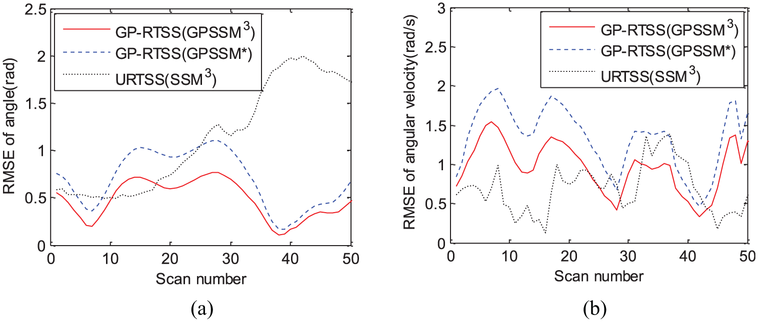
Comparison of state estimation accuracy with GPSSM*, GPSSM3, and traditional SSM3 for pendulum model3 in 100 MC simulations: (a) RMSE of angle and (b) RMSE of angular velocity.

Comparison of state estimation accuracy with GPSSM*, GPSSM4, and traditional SSM4 for pendulum model4 in 100 MC simulations: (a) RMSE of angle and (b) RMSE of angular velocity.
Figure 16 shows the standard deviation of the smoothed estimation at each iteration of optimizing the GPSSM* by the EM-GP-RTSS to simulate the pendulum model3. When optimizing the GPSSM3 by the EM-GP-RTSS iteratively, the smoothed estimation can also be obtained, whose error constantly decreases and eventually converges.

Standard deviation of smoothed estimation by the EM-GP-RTSS at each iteration: (a) standard deviation of angle and (b) standard deviation of angular velocity.
In the simulation experiment, the convergence condition of the EM-GP-RTSS is set to judge whether the maximum number of iterations is reached. Setting a loose maximum number of iterations can avoid the EM falling into a local optimum and directly control the amount of computation. Because of the operability, it is widely used to solve the MLE problem by the EM.11,13
Conclusion and future works
In this article, for the nonlinear dynamic systems, a novel optimization algorithm for the GPSSM is proposed by combining the EM algorithm with the GP-RTSS algorithm, that is, the EM-GP-RTSS algorithm.
The main works are as follows: first, according to the concept of the GP, a theoretical formulation of the GPSSM is proposed, which is not found in previous references. The description provides a rigorous mathematical basis for the development of the EM-GP-RTSS algorithm. Second, according to the maximum likelihood estimation (MLE) criterion, a GPSSM optimization framework with the EM algorithm is proposed. In the EM algorithm, the unknown system state is considered as the lost data, and the maximization of measurement likelihood function is transformed into that of the CEF. Then, the GP-ADF algorithm and the GP-RTSS algorithm are proposed with the GPSSM defined in this article, in order to calculate the smoothed distribution in the CEF. Finally, the MC numerical integral method is used to obtain the approximate expression of the CEF.
In the simulation experiment, a noise pendulum model is used as a representative of the nonlinear dynamic system to verify the effectiveness of the EM-GP-RTSS algorithm proposed in this article. The noise pendulum model0 is selected as the nonlinear system in the laboratory, whose true states are obtained, and then a GPSSM* is trained to simulate it. The EM-GP-RTSS algorithm is used to optimize the GPSSM* for simulating four pendulum models1–4 to get the GPSSMs1–4. The experimental results demonstrate that the GPSSMs1–4 can estimate the system state of the pendulum models1–4 more accurately than the GPSSM* and can reach the estimation accuracy of the traditional SSM. The one-step prediction distributions from the GPSSMs1–4 have the higher confidence than those of the GPSSM*. The EM-GP-RTSS algorithm is helpful to expand the application scope of the GPSSM from a laboratory environment to a practical non-laboratory environment.
In future research, first, a linear kernel function could be designed to develop a corresponding smoothing algorithm for the GPSSMs. A smoothing algorithm based on importance sampling methods can be used to obtain the nonlinear non-Gaussian smoothed estimation. Second, it is necessary to balance the computational complexity by selecting an appropriate number of particles in the MC numerical integral method. However, the relationship between the number of particles and the accuracy is difficult to determine. In addition to the MC numerical integration method, the fixed-point sampling numerical integration methods, such as based on the unscented transition or the spherical-radial cubature rule, may be adopted. The advantage of fixed-point sampling numerical integration methods is to require the fewer sampling points compared with the MC numerical integration method. Then, we will study how to use the high-degree fixed-point sampling numerical integration method to obtain the high-accuracy approximations for formulas (51) and (52).
Footnotes
Handling Editor: James Brusey
Declaration of conflicting interests
The author(s) declared no potential conflicts of interest with respect to the research, authorship, and/or publication of this article.
Funding
The author(s) disclosed receipt of the following financial support for the research, authorship, and/or publication of this article: This research was supported by the National Natural Science Foundation of China (No. 61472441) and the Equipment Prophecy Foundation of China (No. 61403110304).