Sage Journals: Discover world-class research

Abstract

Surface mount technology is an important process in modern electronic circuit manufacturing. Quality control problems have arisen in this area because of the increased design and processing complexity of electronic circuits. Identifying the cause of a fault shortly after its occurrence is critical; however, human fault analysis is inaccurate and time-consuming. Here, we propose a data analysis method that provides actionable information that can easily be interpreted to facilitate rapid identification of fault cause in surface mount technology. The proposed method divides each input variable into a certain number of partitions, and then, the proportion of faults in a partition is calculated in comparison to the proportion of faults in the entire data set. The analytical results are provided to the user with a list that includes the fault causes and a corresponding density histogram for visualization. Real-world surface mount technology data were employed for a case study, in which raw data were preprocessed into an integrated data set consisting of 14,847 rows and 12,929 columns. The proposed method showed reasonable results in approximately 65 s, and the visualization of the results provided a suitable basis for intuitive interpretation, thus demonstrating the method’s ability to generate an efficient analysis in a practical application.

Keywords

Data mining surface mount technology fault analysis fault cause identification smart manufacturing

Introduction

Surface mount technology (SMT) refers to the set of electronic circuit manufacturing processes by which the electronic components are mounted on the surfaces of printed circuit boards (PCBs).¹ With the increase in electronic circuit density and decrease in the size of the electronic devices, SMT is becoming an essential stage in the electronic packaging process.² SMT includes three main production steps: solder paste printing, component placement, and reflow soldering. In the first step, solder paste is spread on a PCB. And then, electronic components are positioned on the pasted pads on the PCB. Finally, reflow soldering step is conducted to connect the electronic components and PCB by melting the component pins and PCB pads at a high temperature.²

Since the SMT is the last stage in the production of an electronic circuit, the quality of the electronic circuit is determined in this stage. Although SMT can allow faster production, the fault risk can be increased for several reasons: incomplete paste deposition, mis-aligned components, and temperature deviations for the final reflow soldering.³ To achieve a high-quality process, multiple sensors are embedded in each production step to monitor several important parameters, such as temperature and oxygen concentration. Moreover, the following quality control processes are implemented between the main production steps: solder paste inspection (SPI) is conducted after the solder paste printing to inspect the volume of the printed solder paste; automated optical inspection (AOI) is employed after the component placement to verify the alignment of the electronic components on the PCB; in-circuit test (ICT) verifies the current flow after the reflow soldering step; and finally, functional board test (FBT) confirms that the electronic circuit functions as designed in the final product. Nonetheless, in practice, faulty products can pass through the process monitoring and inspection steps before their faults are detected in the final FBT step. This may occur because the cut-off criteria set in each monitoring and inspection step are insufficiently precise or because the fault gradually worsens with each successive processing step. Once a faulty product is detected in the FBT step, process engineers analyze the data from the previous steps to identify the cause of the fault. However, because thousands of variables are measured in the production and inspection steps, these human analysis efforts are often inaccurate and always time-consuming.

In recent years, the implementation of machine learning in smart manufacturing systems has drawn increasing interest, and several research efforts have proposed data-driven approaches to improve quality in manufacturing processes.^4,5 Early studies proposed two major approaches: a qualitative approach that incorporates the knowledge of domain experts and a quantitative approach that employs data-driven methods to predict quality and identify critical factors for identifying faulty products.^6,7 Data-driven approaches are particularly attractive for semiconductor manufacturing because of the hundreds of manufacturing steps and the ever-increasing complexity of electronic circuits.⁸ One study direction employed regression methods to establish a virtual metrology system that predicts quality values without an actual quality metrology process, based on fault detection and classification (FDC) data collected from sensors embedded in the processing and metrology equipment.^9–13 In addition, to overcome the underestimation problems of the regression methods, faulty products can be detected and classified directly by employing novelty detection methods.¹⁴ Jang and Kim¹⁵ proposed a monitoring system to predict the “after clean inspection” value of wafers by using a dynamic time warping and clustering method. Data-driven approaches have widely spread to other manufacturing domains, including rolling mill production,¹⁶ food manufacturing,¹⁷ color filter manufacturing,¹⁸ and home appliances manufacturing.¹⁹

Several studies have investigated data-driven approaches for quality improvement in SMT. One early study employed multiple support vector machines to predict the quality of solder joints from illuminated images and classified the quality of solder joints into several classes: no solder, insufficient, good, and excessive. This method’s classification accuracy was greater than 97% on average.²⁰ Acciani et al.³ proposed a neural network–based method to detect solder joint defects from images of the PCB captured by an ordinary digital camera; this method was experimentally demonstrated to classify five types of solder joints with high accuracy. Subsequently, Acciani et al.² proposed a fuzzy architecture to calculate a global quality index for diagnosing solder joints in five classes: poor, acceptable poor, good, acceptable excessive, and excessive. Yang et al.²¹ proposed a neural network–based method to predict quality in the stencil-printing processes often applied to SMT, employing eight control variables, including stencil thickness, stroke speed, and squeegee pressure, to predict the printed paste volume. However, most of these previous research efforts focused on detecting faults to improve the performance of a single automated inspection step, such as AOI, by using data-driven methods based on digital images or control variables.

To address faults in the SMT system as a whole, the main objective of the study presented in this article was to identify fault causes by analyzing data collected from all of the steps in the SMT process in a short time. In practice, there are three main requirements for fault cause identification: rapid analysis, easy interpretation, and sensitivity to the small ratio of faults. If one type of fault occurs consecutively during manufacturing, the online system should identify the fault causes rapidly; however, the types of faults change each time. Hence, the fault cause identification system is required to analyze a factory-wide data within a few minutes for online identification. In addition, the easy interpretation of the analytical result is essential for obtaining actionable information in a practical fault analysis framework.¹⁹ When the analysis identifies a fault cause, process engineers must determine the exact range of values indicating the selected feature causing the fault. Moreover, because the fault ratio in SMT processes is less than 1%, the fault cause identification method should not overlook this small ratio.

In this article, we propose a data-driven method to identify fault causes with a factory-wide data analysis of the SMT process. For easy interpretation, the result of the proposed method is designed to be obtained as not only causal variables but also their corresponding fault-inducing value ranges. To identify fault causes for a small ratio of faults, the proposed method employs the concept of lift. That is, the proposed method first partitions each variable according to its respective value ranges and then applies a lift value to calculate the ratio of the number of faults in a certain partition to that in the entire data set. Finally, the casual variables together with the corresponding fault-inducing values with large lift values are visualized as a graph for easier interpretation and further analysis. Moreover, the proposed method does not require any training stages, thus enabling a rapid analysis, as demonstrated by a case study conducted using real-world SMT data collected from the processing and inspection steps. The main contributions for this article can be summarized as follows:

The proposed method is a light-weight method for online operation.

The result of the proposed method is formed as causal variables and their corresponding fault-inducing value ranges.

The proposed method calculates the lift values for class-imbalanced datasets.

The case study is conducted with a real-world factory-wide SMT dataset.

Related work

One of the main research directions for fault cause identification in manufacturing is the feature selection–based approach. The basic idea of feature selection–based approaches is that a small subset of input variables used to construct an accurate quality prediction model can be fault causes. Malhi and Gao²² proposed a principal component analysis (PCA)-based feature selection method for bearing condition controlling, through which most contributed features were selected for the eigenvector with the largest corresponding eigenvalue after employing PCA for the original features. Li et al.²³ proposed two more indices for the result of PCA: the improved weighted contribution and sensor validity index. This method focused on an unsupervised identification of faulty sensors. Rokach and Maimon¹⁷ proposed an ensemble-like breadth-oblivious-wrapper (BOS) algorithm. During the construction of an oblivious decision tree, the algorithm searches the best decomposition structure of features to maximize F-measure through iterations, and each oblivious decision tree contains a decomposed feature subset, which are mutually exclusive from the others. This method results in high prediction performances for class-imbalanced datasets. However, as it is a wrapper approach, the training time complexity is relatively high. Kang et al.²⁴ proposed a heuristic outlier-insensitive hybrid feature selection (OIHFS) method which focuses on outliers contained in a dataset to improve the prediction performance; they applied the method to detect rolling elements bearing faults. OIHFS employed both wrapper and filter approaches to obtain better prediction performance and computational efficiency. Kang et al.²⁴ also employed sequential forward floating search and outlier-considered feature assessment metric to improve the classification performance of k-fold k-nearest neighbor classifier. However, because of the training efficiency, the experiments were conducted on only tens of features and data points. Kang et al.²⁵ proposed a random forward search-based wrapper method for virtual metrology in semiconductor manufacturing. To reduce the training time complexity of step-wise search, the authors divided the original features into m number of disjoint feature sets and conducted forward and backward searches. This method results in efficient performance for experiments with real-world virtual metrology data. These approaches have been widely applied to several domains. However, one major drawback of these feature selection–based approaches is that they do not identify the value ranges at which the selected variables result in a fault; this is a critical information in practical applications. Although decision tree–based approaches can extract explicit rules, the refined rules usually consist of numerous factors that can trigger an action in real-world applications. In addition, such approaches employ learning models that require large balanced datasets and are therefore time-consuming.

Another research direction is to identify fault causes by extracting informative features from variables. According to Xu et al.,²⁶ the performance of conventional feature selection approaches based on accuracy tends to degrade when they are applied to class-imbalanced problems. Therefore, Xu et al.²⁶ applied the E-algorithm extended from fuzzy classification to fault cause identification in a power distribution system by using imbalanced data. They extracted features with the idea of support and confidence to calculate the relationship between fault and each input variable; however, they did not consider the lift value. A histogram-based method can be included in this area. One major advantage of this method is that continuous sensor values can be summarized into a certain number of discrete bins through a histogram. Sakthivel et al.²⁷ employed a histogram-based method to extract features from a time-series vibration signal. They then used a decision tree model to select important features from among the extracted discrete features. Sugumaran and Ramachandran²⁸ also employed the histogram-based feature extraction and decision tree–based feature selection, but added a rule-based classifier to obtain fault diagnosis of the roller bearing from the time-series sensor values. Lin and Huang²⁹ extended the idea of a histogram-based method and extracted nine statistical features, such as mean, standard deviation, and kurtosis, from the histogram of vibration signals to train a fuzzy-based classifier. However, the histogram-based method cannot directly be applied to problems comprising variables other than time-series variables. Moreover, the final feature selection stage is still time-consuming for a large-sized dataset with more than thousands of rows and columns.

Proposed method

Data sources

In SMT processes, manufacturing data can be collected from multiple sensors embedded at each production and inspection location. The process data can be collected during the reflow soldering step, which consists of heating, retained high temperature, and cooling stages. Time-series data that measure changes in temperature over time are collected. Data can also be collected from the SPI, AOI, ICT, and FBT steps. Data from SPI include the volume, height, width, and offsets of the printed solder paste at hundreds of sampled points on each PCB. Data from AOI include the position of each electronic component recorded in X–Y coordinates. Data from ICT include the amount of current flowing at each electronic component connected to the PCB. Data from FBT indicate whether the electronic circuit is functioning as designed in the final product; therefore, these data should be used as output variables. In contrast, the sensors employed in reflow soldering, SPI, AOI, and ICT monitor the SMT processes, and therefore, the generated data should be used as input variables. Each input variable from the entire SMT process can be a fault cause candidate, and certain environmental variables, such as humidity, dust level, and temperature in the facility, can also be collected and used as input variables to investigate the full range of fault cause candidates.

Calculation of lift value to identify fault cause

The main purpose of the proposed method is to identify fault causes over the entire SMT process. The analytical results should be easy to interpret and obtained in almost real time. To ease interpretation, we designed the proposed method to derive causal variables along with the corresponding fault-inducing values. For example, if a fault occurs when the starting temperature in the reflow soldering step exceeds 190°C, the more informative result of the proposed method would pair the variable name and value, for example, {Variable: Starting temperature; Value: Over 190°C}. To enable a fast analysis, the proposed method is designed to derive the analytical results without needing to train a complex model.

The proposed method first divides each variable into k sequential partitions according to its value range. If the value range of an integer input variable is [91,120] and k is set to 10, the input variable will be partitioned into 10 areas, each with a range of three: [91,93], [94,96], . . ., [117,120]. The proposed method considers each partition of each variable as an independent fault cause candidate. Thus, if the number of input variables is 100,000 and k is set to 10, then 1,000,000 independent candidates will be analyzed.

The next step is the calculation of lift values. The basic idea of a lift value in data mining was introduced through a study on association rule mining, which was proposed to identify relationships between items in a set.³⁰ Here, we employed the concept of lift values to compare the proportion of an item in a set with that of the item in all sets. First, we prepared $p_{ij}$ , the $j th$ partition of the $i th$ input variable, for all i and j. Support value, $S (p_{ij})$ , can be obtained by dividing the number of faults in $p_{ij}$ by the number of both faults and normal products in the set of all data, D; thus, $S (p_{ij})$ indicates the probability of faults caused by $p_{ij}$ relative to D. Confidence value, $C (p_{ij})$ , can then be obtained by dividing $S (p_{ij})$ by the proportion of the number of data in $p_{ij}$ to the number of data in D; thus, $C (p_{ij})$ indicates a conditional probability of faults for given $p_{ij}$ . Finally, lift value, $L (p_{ij})$ , can be obtained by dividing $C (p_{ij})$ by the proportion of the number of faults in the entire data to the number of data in D; thus, $L (p_{ij})$ indicates the proportion of the probability of faults in $p_{ij}$ to the probability of faults in D. If $L (p_{ij}) = 1$ , the $i th$ partition does not affect the fault at all. If $L (p_{ij}) > 1$ , the variable and corresponding value range may be a fault cause. Hence, the larger the value of $L (p_{ij})$ , the greater is the probability that the given variable and partition represent a fault cause.

Reporting the analytical results

The proposed method provides lift value, $L (p_{ij})$ , for all combinations of input variables and their partitioned value ranges. By treating all the combinations as independent fault cause candidates, the $i \times j$ number of lift values was sorted together regardless of which j belonged to which i. As larger lift values indicate higher fault cause probabilities, the analytical results should be reported by sorting all lift values in the descending order. A graphic visualization of the causal variables can then be provided to compare the fault cause probabilities of the different variables. Here, we recommend a density histogram to compare the proportion of faults and normal products in one figure for a variable, as illustrated in the following case study. The overall algorithm, including partitioning and lift value calculation, is summarized in Figure 1.

Figure 1.

The algorithm of the proposed method.

Real-world case study

Overview

A case study was conducted to validate the proposed method on a set of real-world SMT process data collected from one of the largest smart junction box (SJB) manufacturers in South Korea. SJBs play a key role in controlling electronic parts in automobiles and are therefore a critical component affecting consumer satisfaction. The case study followed a common data mining process: data acquisition, data preprocessing, analytical modeling, and reporting with visualization, as shown in Figure 2. The case study was conducted using R-Studio with R version 3.3.2 on a personal computer with an Intel(R) i7–6400k processor and 32 GB of memory.

Figure 2.

Data analytics process.

Data acquisition

The data were collected from an actual SMT process for producing SJBs. The SMT process for the case study included all of the aforementioned production and inspection steps, as shown in Figure 3, including reflow soldering, SPI, AOI, ICT, and FBT steps. As data cannot be acquired directly from some production steps, such as solder paste printing and component positioning, we utilized data collected from their corresponding inspection steps. In addition, two external datasets were collected to represent environmental factors: weather and dust. Data were collected in May 2017, and the raw data collected from each SMT process were not preprocessed. The total amount of data is more than 100 million rows. In practice, factory-wide data collected through multiple sensors from all the SMT processes are difficult to organize as one dataset and transfer to another location. The dataset used in this case study may have some limitations but is large enough to evaluate the idea of the proposed method. The sizes of the raw datasets are summarized in Table 1.

Figure 3.

SMT process in the case study.

Table 1.

Size of collected raw data.

Step	No. of rows	No. of columns
Reflow soldering	1,130,863	37
SPI	52,627,468	39
AOI	35,235,513	18
ICT	47,629,882	34
FBT	11,518,870	13
Weather	13,320	8
Dust	10,149	7

SPI: solder paste inspection; AOI: automated optical inspection; ICT: in-circuit test; FBT: functional board test.

Data preprocessing

In practice, data sources and types are heterogeneous and should be integrated through preprocessing.³¹ As shown in Table 1, the raw data collected from each step are quite different. As the raw data from each step are not organized according to the product, the number of rows is related to the number of products inspected at the inspection step multiplied by the number of components to be inspected at a particular step. For example, approximately 1450 components were inspected for each of the approximately 37,000 products during the SPI step. Hence, the number of rows for this step is more than 50 million, and thus, each product is represented in multiple rows in the raw data. To construct an integrated dataset for analysis, each product must have only one row containing multiple variables, and all data tables should be joined by considering the product as key. Therefore, we preprocessed raw data to construct an integrated dataset through three main stages: data pivoting, summarization of values, and derivation of new variables.

Data pivoting is the process of transforming multiple product rows into multiple columns so that each product has only one row vector. For example, the SPI data contain approximately 1,450 inspection components for each product. For each inspection component, several values, such as volume, height, and offset on the X- and Y-axes, are measured. The raw data should be transformed so that each measured value for each inspection component is an input variable for each product. Hence, the number of input variables in the pivoted data is the number of all combinations of inspection components and their corresponding measurements, as illustrated in Figure 4.

Figure 4.

An example of data pivoting.

The summarization of values is often employed if statistical information for the original input values is useful. For example, temperature and oxygen concentration are measured in millisecond intervals during the reflow soldering step. If we pivot each data point for each variable, three major drawbacks occur: the number of input variables increases considerably, the slight fluctuations in the time-series data are not smoothed, and small differences in the time axes of the different products are reflected in the data. In such cases, statistically summarized values are preferred. Therefore, for the reflow soldering step, we divided the processing time into several sections, including idling, heating, temperature maintenance, and cooling, as advised by process experts. The raw data can then be summarized according to the average and standard deviation of each section, as illustrated in Figure 5.

Figure 5.

An example of summarization of values.

The derivation of new variables is employed to create additional information from the original variables. In some cases, the small piece of information conveyed by each original variable is not useful by itself. In contrast, a derivative variable can contain useful information for analysis. For example, the environmental data representing the weather, humidity, and dust level were measured once every hour during the SMT process. Although the environmental information is useful, the raw data collected over time cannot be employed directly. Hence, we created new variables, for example, binary variable, to indicate whether it was raining during each step, and numerical variable, indicating the maximum dust level during all steps, as shown in Figure 6. As another example, the AOI step comprised two pieces of inspection equipment, and because the inspection precision of each equipment type can be different, a new variable indicating whether each product passed the equipment’s inspection was added.

Figure 6.

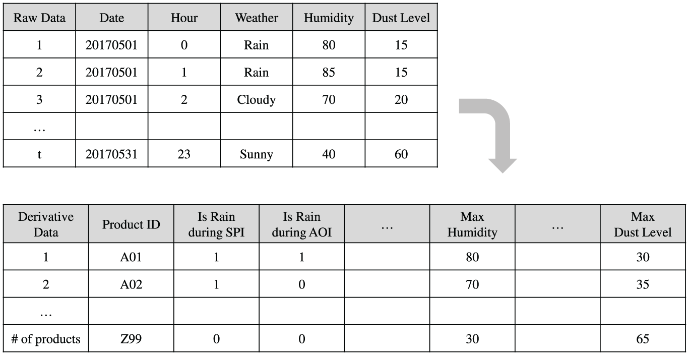
An example of derivation of new variables.

After these preprocessing steps, all data organized by products were integrated into one dataset to be analyzed. Other commonly used preprocessing steps were also employed: data with missing or outlying values were eliminated along with uninformative variables with zero-deviation or index information. The final integrated dataset consists of 14,847 products and 12,929 input variables.

Analytical modeling

To identify the fault causes, we defined the fault from the output variables in the raw data. As the FBT step is the final step to confirm the quality of each product, we employed the FBT data to define faults. In this case study, FBT was applied to identify 757 types of faults, such as input/output current under the switch-off condition and the amount of signal under a load test. We selected the three most common types of faults to be analyzed defined only as $F 1$ , $F 2$ , and $F 3$ in this study, as their identities are confidential and therefore cannot be disclosed. However, the faults are indicated based on the inspection results from a headlamp load test, a signal operation test under load, and a static bending load test, respectively. If a measured value from FBT falls outside the predefined specification range, the product is classified as a fault. Among 14,847 products, the numbers of faulty products of each type were 10, 9, and 6, respectively, with corresponding fault ratios of 0.067%, 0.060%, and 0.040%. As the data were highly class-imbalanced, conventional analytical methods based on the fault ratio ignore these faults. In contrast, the proposed method calculates the lift values to compare the fault ratio in a given partition to the expected fault ratio. By dividing each variable into 10 sequential partitions based on its corresponding value ranges, we obtained 12,929 input variables and 129,290 partitions, each representing an independent fault cause candidate. For each output variable, $S (p_{ij})$ , $C (p_{ij})$ , and $L (p_{ij})$ were calculated for all partitions, as shown in Figure 1. Finally, we eliminated results from partitions where the $L (p_{ij}) < 1$ and sorted all remaining results according to $L (p_{ij})$ in the descending order. The number of partitions, k, which is set manually, decides how precisely each variable is divided. If k is small, the computational cost is low, but the precision is also low. If k is large, the computational cost is high but the result can be more precise. Although the determination of k must also be considered, a predetermined value of k was preferred for efficiency. We set the default value of k to be 10 for the following experiment based on another literature considering sequential partitioning.³²

Reporting and visualization

One of the purposes of the proposed method is to provide actionable information that can be easily interpreted. Therefore, the proposed method provides both the list of causes and a density histogram to illustrate these causes. This section presents the analytical results for the three types of faults in the case study described earlier.

Table 2 shows the top 12 lift values generated by the proposed method for $F 1$ . The columns of Table 2 indicate the name of the input variables; the low and high limits for the selected partition; the number of faulty and normal products in the partition; and the support, confidence, and lift values for the partition. The names of the input variables were converted to numeric codes to maintain confidentiality. Through the columns indicating the low and high limits for the selected partition, the process engineers can easily identify the fault-inducing value ranges of the causal variables. Then, the number of faulty and normal products in the partition can also be checked. The support and confidence values calculated for each partition are placed next. As mentioned earlier, support and confidence values did not have significant information when they are used for class-imbalanced problems, where the ratio of faults is extremely small. They were only used to calculate the lift values, which contain the most important information. As shown in Table 2, the highest lift value for a partition was greater than 16, indicating that the probability of faults occurring in this partition was 16 times greater than that in the overall data. In addition, ICT components 172 and 173 were identified as causes. As the similar numeric codes indicate similar inspection types, these ICT inspection measurements were considered critical causes of $F 1$ . Figure 7 presents density histograms of the top four results for visualization; the red bars indicate faults and the shaded bars indicate normal products from the perspective of the selected variable. Because the proportion of faults is very small, we recommended using the density histograms or any other type of scaled graph. As shown in Figure 7, the faults and normal products exhibited very different densities. For “ICT_173_VALUE,” the fault ratio dramatically increased between approximately 12.5 and 13, whereas the normal products were distributed near approximately 9.5 or 12.2. The table and corresponding figures also facilitate easy identification of the fault-inducing value ranges of the other three variables, demonstrating the proposed method’s utility to process engineers who can quickly act on the generated probabilities to confirm the fault causes.

Table 2.

Analytical results for $F 1$ (resulted in 65.71 s).

Input variable	Range_low	Range_high	N_fault	N_normal	Support	Confidence	Lift
ICT_173_VALUE	12.524	12.947	5	449	0.00034	0.01101	16.35
ICT_172_VALUE	12.608	13.039	5	453	0.00034	0.01092	16.21
ICT_57_VALUE	125012	128244	10	960	0.00067	0.01031	15.31
SPI_VALUE_SD_VOLUME_PER_819	114.8426	119.6029	5	529	0.00034	0.00936	13.90
SPI_VALUE_SD_OFFSETY_MM_539	−0.0967	−0.0774	7	866	0.00047	0.00802	11.90
SPI_VALUE_SD_VOLUME_PER_409	139.505	144.173	7	878	0.00047	0.00791	11.74
SPI_VALUE_SD_AREA_PER_539	108.1984	110.1836	5	674	0.00034	0.00736	10.93
SPI_VALUE_SD_HEIGHT_UM_409	195.7305	200.7226	6	824	0.0004	0.00723	10.73
SPI_VALUE_SD_HEIGHT_UM_539	193.9446	200.5157	9	1479	0.00061	0.00605	8.98
SPI_VALUE_SD_OFFSETY_MM_527	−0.1422	−0.1204	6	994	0.0004	0.006	8.91
SPI_VALUE_SD_HEIGHT_UM_129	194.551	199.4554	5	844	0.00034	0.00589	8.74
SPI_VALUE_SD_AREA_PER_449	107.3986	109.4227	6	1054	0.0004	0.00566	8.40

Figure 7.

Visualization of the results for $F 1$ : (a) ICT_173_VALUE, (b) ICT_172_VALUE, (c) ICT_57_VALUE, and (d) SPI_VALUE_SD_VOLUME_PER_50.

Table 3 shows the top 12 lift values generated by the proposed method for $F 2$ . Interestingly, the analytical results for $F 2$ were relatively different from those for $F 1$ . For $F 2$ , the environmental variables that measured the temperature and humidity were at the top of the sorted list. This result may indicate that the reliability of the facility’s air-conditioning may affect the occurrence rate of $F 2$ and further effort may be required to maintain constant environmental conditions to prevent the occurrence of this type of fault. Figure 8 presents the density histogram for four types of variables, showing that the faults and normal products were distributed differently. In addition, the measured values for “ICT_352_VALUE” over $0.725$ may further impact the occurrence of $F 2$ .

Table 3.

Analytical results for $F 2$ (resulted in 65.22 s).

Input variable	Range_low	Range_high	N_fault	N_normal	Support	Confidence	Lift
TEMP_AOI	21.35	24.4	6	1138	0.0004	0.00524	8.65
HUMID_RE	37.6	47	7	1418	0.00047	0.00491	8.10
TEMP_RE	21.35	24.4	6	1231	0.0004	0.00485	8.00
HUMID_ICT	56.4	65.8	7	1441	0.00047	0.00483	7.97
SPI_VALUE_SD_OFFSETX_MM_645	−0.0187	−0.0106	5	1044	0.00034	0.00477	7.86
HUMID_MEAN	46.3	55.56	6	1265	0.0004	0.00472	7.79
ICT_352_VALUE	0.7244	0.7332	7	1569	0.00047	0.00444	7.33
HUMID_SPI	56.4	65.8	7	1583	0.00047	0.0044	7.26
SPI_VALUE_SD_OFFSETX_MM_1115	0.0229	0.0332	5	1144	0.00034	0.00435	7.18
ICT_430_DEVIATION	−8.58	−5.56	5	1161	0.00034	0.00429	7.07
HUMID_AOI	37.6	47	6	1399	0.0004	0.00427	7.04
ICT_430_VALUE	52,102	53,824	5	1182	0.00034	0.00421	6.95

Figure 8.

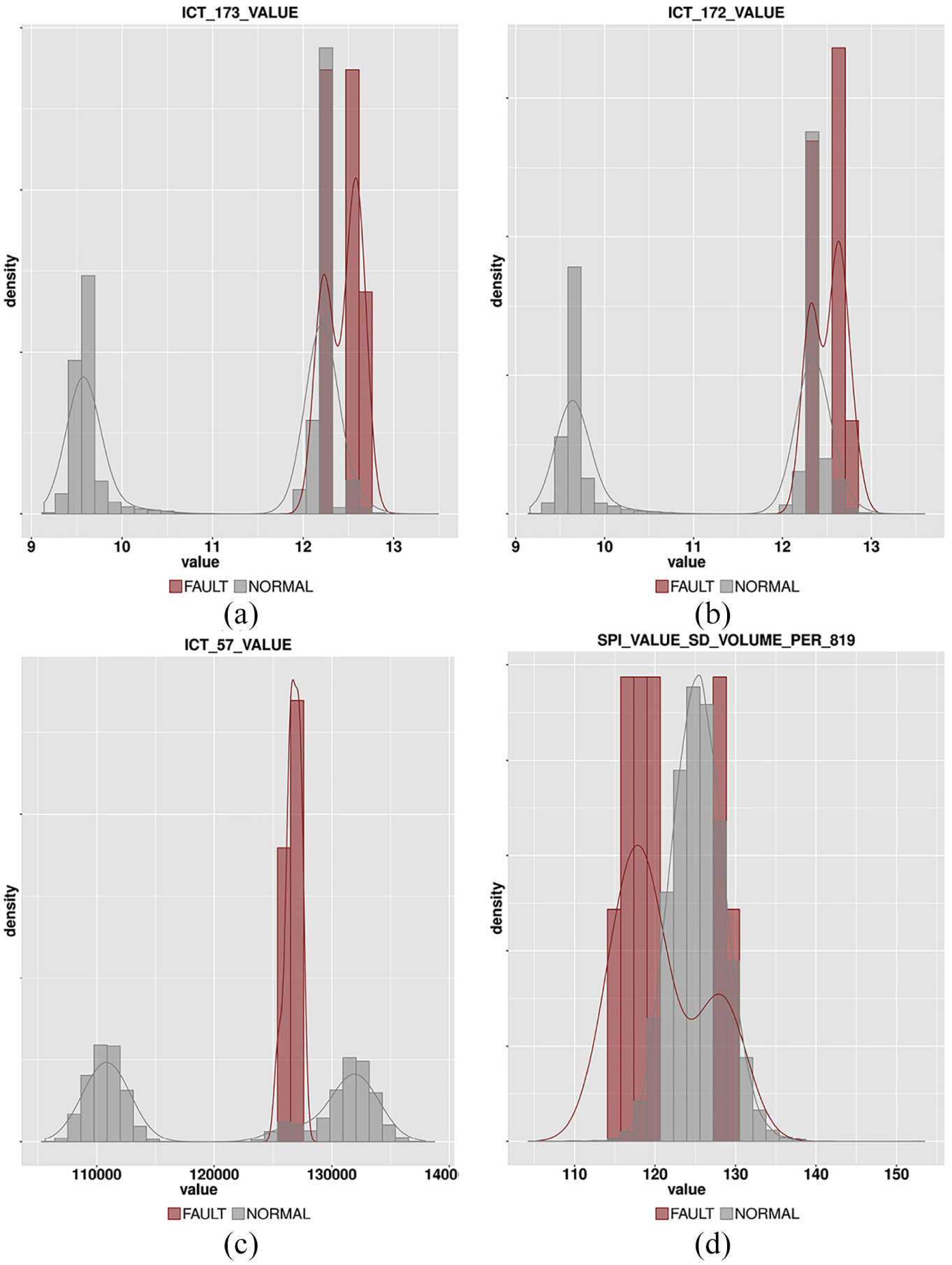
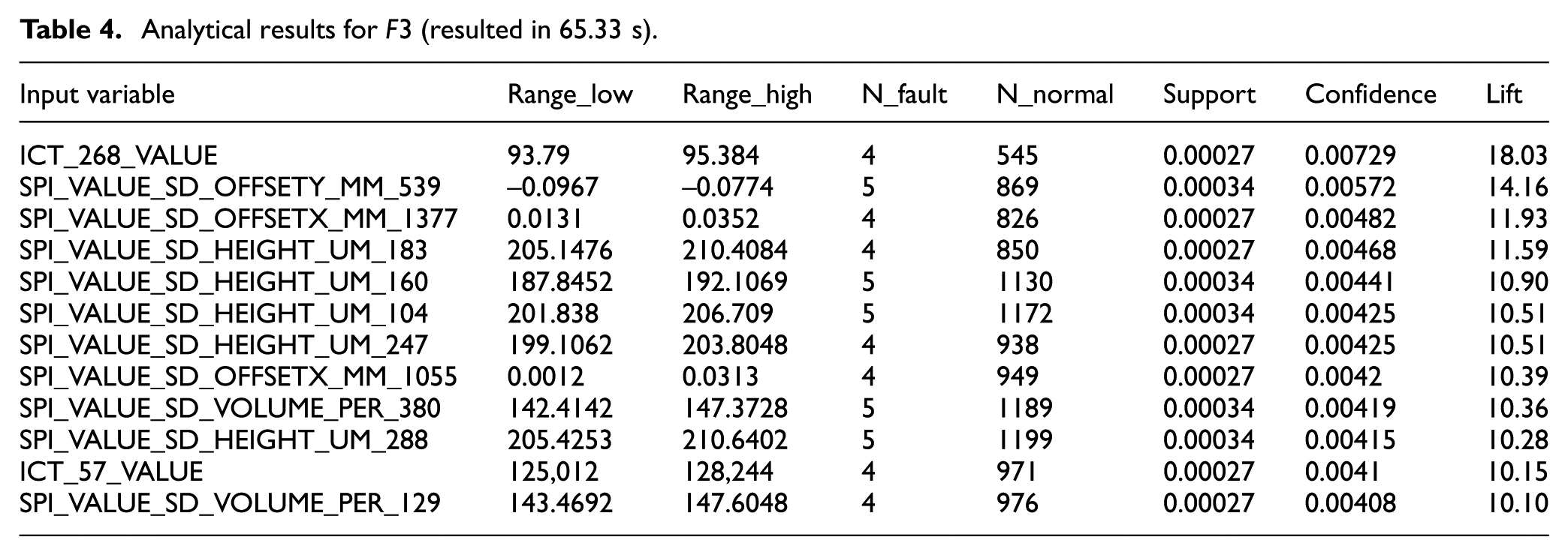
Visualization of the results for $F 2$ : (a) TEMP_AOI, (b) SPI_VALUE_SD_OFFSETX_MM_645, (c) HUMID_MEAN, and (d) ICT_352_VALUE.

Table 4 shows the top 12 lift values generated by the proposed method for $F 3$ . Here, “ICT_268_VALUE” was identified as the most critical fault cause. As shown in Figure 9(a), the normal products were distributed near approximately 103, whereas the faults were distributed near approximately 95. We can conclude that the 268th ICT component was the main cause of $F 3$ . The second highest lift value was generated in the “SPI_VALUE_SD_OFFSETX_MM_539” category. The comparison of the histograms in Figure 9(b) shows that the fault values are distributed more widely than normal products values. The measured value near $- 0.10$ for this variable may be one of the main causes of $F 3$ .

Table 4.

Analytical results for $F 3$ (resulted in 65.33 s).

Input variable	Range_low	Range_high	N_fault	N_normal	Support	Confidence	Lift
ICT_268_VALUE	93.79	95.384	4	545	0.00027	0.00729	18.03
SPI_VALUE_SD_OFFSETY_MM_539	–0.0967	–0.0774	5	869	0.00034	0.00572	14.16
SPI_VALUE_SD_OFFSETX_MM_1377	0.0131	0.0352	4	826	0.00027	0.00482	11.93
SPI_VALUE_SD_HEIGHT_UM_183	205.1476	210.4084	4	850	0.00027	0.00468	11.59
SPI_VALUE_SD_HEIGHT_UM_160	187.8452	192.1069	5	1130	0.00034	0.00441	10.90
SPI_VALUE_SD_HEIGHT_UM_104	201.838	206.709	5	1172	0.00034	0.00425	10.51
SPI_VALUE_SD_HEIGHT_UM_247	199.1062	203.8048	4	938	0.00027	0.00425	10.51
SPI_VALUE_SD_OFFSETX_MM_1055	0.0012	0.0313	4	949	0.00027	0.0042	10.39
SPI_VALUE_SD_VOLUME_PER_380	142.4142	147.3728	5	1189	0.00034	0.00419	10.36
SPI_VALUE_SD_HEIGHT_UM_288	205.4253	210.6402	5	1199	0.00034	0.00415	10.28
ICT_57_VALUE	125,012	128,244	4	971	0.00027	0.0041	10.15
SPI_VALUE_SD_VOLUME_PER_129	143.4692	147.6048	4	976	0.00027	0.00408	10.10

Figure 9.

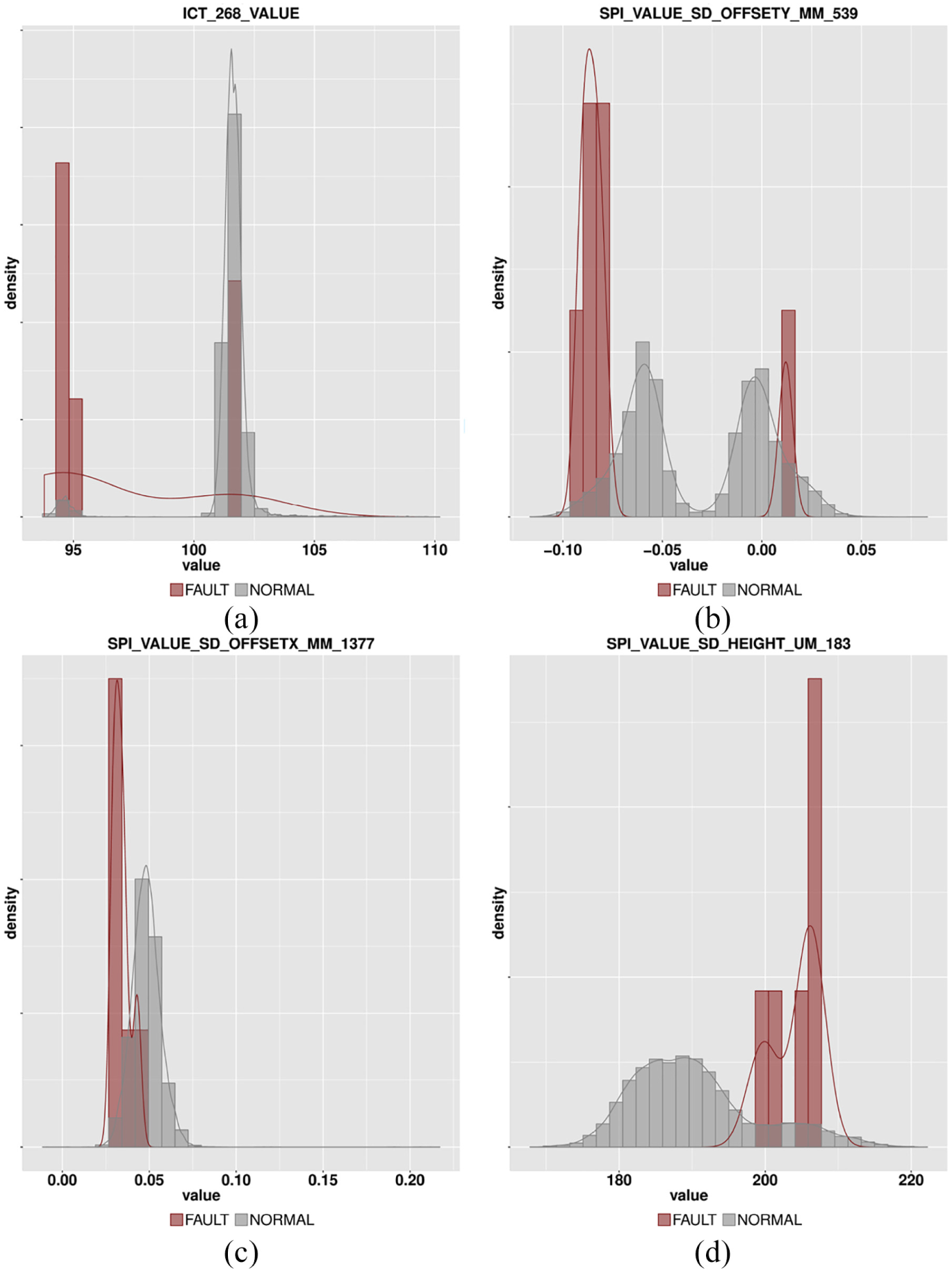
Visualization of the results for $F 3$ : (a) ICT_268_VALUE, (b) SPI_VALUE_SD_OFFSETX_MM_539, (c) SPI_VALUE_SD_OFFSETX_MM_1137, and (d) SPI_VALUE _SD_HEIGHT_UM_183.

For comparison, we selected the two most representative benchmark methods: PCA-based method²² and decision tree–based method.²⁸ For the PCA-based method, we obtained one eigenvector with the largest eigenvalue, and then, the most contributed original variables for that eigenvector were selected. For the decision tree–based method, the histogram-based feature extraction was not used because the variables in the dataset were not time-series variables. We trained a decision tree, and the variables used in the branch of the decision tree were selected as important variables.

Table 5 shows that the data analysis time for each method, with the preprocessed dataset having 14,847 examples and 12,929 variables. As PCA is an unsupervised method, the analysis time is the same for each type of fault. The decision tree-based method did not work for $F 2$ and $F 3$ . We tried to decrease the minimum number of data in a leaf node of the decision tree to 2; nevertheless, the result of the decision tree was just a stump for $F 2$ and $F 3$ . Therefore, we conclude that the decision tree–based method tends to overlook the small ratio of faults. As shown in Table 5, the analysis time of the proposed method is much smaller than those of other benchmark methods. The proposed method required 65 s roughly, while the PCA-based method and decision tree-based method required 6629 and 276 s, respectively. We also compared the data analysis time of the proposed method with a larger k value. When k increased to 20, the data analysis time increased to approximately 111 s, which was still comparable. The data analysis time of the proposed method follows the number of partitions at most. Therefore, the proposed method can be preferred for a real-time system.

Table 5.

Data analysis time for each method (in seconds).

Fault	PCA-based	Tree-based	Proposed (k = 10)	Proposed (k = 20)
F1		276.47	65.71	110.92
F2	6629.90	N/A	65.22	111.31
F3		N/A	65.33	111.87

PCA: principal component analysis.

For the PCA-based method, the first principal component contains 22.27% of the variance of original variables. We selected the four most contributed variables to this component. Figure 10 shows the density histogram of the selected four variables and the target is selected to be $F 1$ for visualization. Compared to the results of the proposed method, the selected variables in the PCA-based method had less power to explain the difference between the faults and normal products. The density functions of the normal products and faults mostly overlapped. In addition, the PCA-based method could not point the fault-inducing value ranges.

Figure 10.

Visualization of the results of PCA-based method for $F 1$ : (a) SPI_VALUE_SD_AREA_PER_17, (b) SPI_VALUE_SD_AREA_PER_1412, (c) SPI_VALUE_SD_AREA_PER_20, and (d) SPI_VALUE_SD_AREA_PER_19.

Figure 11 shows the results from decision tree–based method for $F 1$ , which was the only available result for all fault types. This method was not sensitive to the small ratio of faults. Decision tree–based method distinguished only one acceptable region (the upper left region in Figure 11(b)), but tended to ignore other faults when they occupied a small proportion for a region.

Figure 11.

Visualization of the results of decision tree–based method for $F 1$ : (a) the constructed tree with two variables used in the branch and (b) the corresponding 2D plot with decision boundaries (horizontal and vertical lines) for faults (red) and normal products (black).

In summary, the proposed method identified a list of causal variables and their corresponding fault-inducing value ranges for all three types of faults. In addition, the proposed method required only approximately 65 s for each analysis, enabling rapid analysis of factory-wide SMT data. The proposed method identified different causes for each type of fault and provided density histograms for easy visualization. In contrast, the PCA-based method and decision tree–based method required more time than the proposed method. In addition, the PCA-based method was not able to identify the fault-inducing value range, and the decision tree–based method was not sensitive to the small ratio of faults and only one result was obtained for three fault types. Although we illustrated only four figures for each type of fault, the real-world system can provide figures corresponding to all fault cause candidates generated by the proposed method. The process engineers confirmed that the identified variables and the corresponding value ranges would be the actual fault causes.

Conclusion

In this article, we proposed a data-driven method to identify fault causes in SMT processes, which have become increasingly complex and thus more vulnerable to inaccurate and time-consuming human inspection. The main purpose of the proposed method is to identify both the fault-inducing variable and its corresponding value range to facilitate interpretation and generate actionable information. First, the proposed method divides each variable into k sequential partitions based on the variable’s value range. Each partition of each variable is treated as an independent fault cause candidate. The lift value of each candidate is then calculated to compare the proportion of faults in that partition to that present in the entire dataset. The analytical results provide list of variables sorted by the lift values and density histograms for easy visualization.

The proposed method was applied to a case study employing real-world SMT process data. We preprocessed the raw data to construct an integrated data set for analysis through data pivoting, summarization of values, and derivation of new variables. Three of the most frequent types of faults were selected for analysis; however, the numbers of fault occurrences in these categories were very small, at 10, 9, and 6 faults, respectively. The proposed method showed reasonable fault cause identification results and the visualizations provided an intuitive basis for easy interpretation. In addition, the analytical process required only approximately 65 s, guaranteeing a fast fault cause analysis, reducing the time and effort required for process engineers to investigate further to confirm the results. The comparison with benchmark methods (PCA and decision tree) showed that the proposed method resulted in the fastest analysis time and was robust to the small ratio of faults. This method can easily be developed as a computer program without any prior knowledge of sophisticated data mining methods.

The proposed method has some limitations that need further research. First, the proposed method focuses on identifying each fault cause candidate independently to facilitate interpretation and efficiency. However, two or more causes may simultaneously affect fault occurrences. Therefore, one further research direction could be to develop a method of calculating lift values for two or more variable–partition combinations. Second, the proposed method analyzed the case study data, including 14,847 products, 12,929 variables, and 10 partitions, in almost real time. However, to apply this method to larger datasets, a more efficient method for calculating lift values should be developed, such as the Apriori algorithm³⁰ used for association rule mining. In addition, the determination of the partitioning parameter k can be studied. A stochastic approach to vary k for variance of input variable may improve the proposed method. Finally, we collected data for only 1 month in this case study, and thus, we neglected variables, such as seasonal effects or changes of the amount of throughput, that affect quality over time. Therefore, we intend to conduct a new case study with SMT data collected over a year to identify the effects of such variables.

Footnotes

Handling Editor: Pavel Stasa

Declaration of conflicting interests

The author(s) declared no potential conflicts of interest with respect to the research, authorship, and/or publication of this article.

Funding

The author(s) disclosed receipt of the following financial support for the research, authorship, and/or publication of this article: This work was supported by funding from Chungnam National University. This work was also supported in part by the Yura Co., Ltd. (2018-0280-01), Korea Institute of Industrial Technology (2018-1348-01), and the Industry Core Technology Development Program (10073136) funded by the Ministry of Trade, Industry, and Energy of Korea (MOTIE).

ORCID iD

Seokho Kang

References

Prasad

Surface mount technology: principles and practice. Berlin: Springer Science & Business Media, 2013.

Acciani

Fornarelli

Giaquinto

A fuzzy method for global quality index evaluation of solder joints in surface mount technology. IEEE T Ind Inform 2011; 7(1): 115–124.

Acciani

Brunetti

Fornarelli

Application of neural networks in optical inspection and classification of solder joints in surface mount technology. IEEE T Ind Inform 2006; 2(3): 200–209.

Köksal

Batmaz

Testik

MC.

A review of data mining applications for quality improvement. Expert Syst Appl 2011; 38: 13448–13467.

Wang

Wan

et al . Implementing smart factory of industrie 4.0: an outlook. Int J Distrib Sens N 2016; 12(1): 3159805.

Venkatasubramanian

Rengaswamy

Kavuri

SN.

A review of process fault detection and diagnosis: part II: qualitative models and search strategies. Comput Chem Eng 2003; 27: 316–326.

Venkatasubramanian

Rengaswamy

Yin

et al . A review of process fault detection and diagnosis: part I: quantitative model-based methods. Comput Chem Eng 2003; 27: 291–311.

Kang

Kim

Cho

Semi-supervised support vector regression based on self-training with label uncertainty: an application to virtual metrology in semiconductor manufacturing. Expert Syst Appl 2016; 51: 85–106.

Cheng

. Application development to virtual metrology in semiconductor industry. In: Proceedings of the 31st annual conference of IEEE Industrial Electronics Society, Raleigh, NC, 6–10 November 2005, pp.124–129. New York: IEEE.

10.

Chang

Kang

Hsu

et al . Virtual metrology technique for semiconductor manufacturing. In: Proceedings of the 2006 international joint conference on neural networks, Vancouver, BC, Canada, 16–21 July 2006, pp.5289–5293. New York: IEEE.

11.

Besnard

Toprac

. Wafer-to-wafer virtual metrology applied to run-to-run control. In: Proceedings of the 3rd ISMI symposium on manufacturing effectiveness, Austin, TX, October 2006.

12.

Kang

Lee

Cho

et al . A virtual metrology system for semiconductor manufacturing. Expert Syst Appl 2009; 36(10): 12554–12561.

13.

Kang

Kim

Lee

et al . Virtual metrology for run-to-run control in semiconductor manufacturing. Expert Syst Appl 2011; 38(3): 2508–2522.

14.

Kim

Kang

Cho

et al . Machine learning-based novelty detection for faulty wafer detection in semiconductor manufacturing. Expert Syst Appl 2012; 39(4): 4075–4083.

15.

Jang

Kim

GY.

A monitoring method of semiconductor manufacturing processes using internet of things-based big data analysis. Int J Distrib Sens N 2017; 13(7): 1550147717721810.

16.

Lieber

Stolpe

Konrad

et al . Quality prediction in interlinked manufacturing processes based on supervised & unsupervised machine learning. Proc CIRP 2013; 7: 193–198.

17.

Rokach

Maimon

Data mining for improving the quality of manufacturing: a feature set decomposition approach. J Intell Manuf 2006; 17: 285–299.

18.

Tsai

Lee

CY.

Data mining for yield improvement of photo spacer process in color filter manufacturing. Proc Manuf 2017; 11: 1958–1965.

19.

Kang

Kim

Shim

et al . Mining the relationship between production and customer service data for failure analysis of industrial products. Comput Ind Eng 2017; 106: 137–146.

20.

Yun

Sim

Kim

Support vector machine-based inspection of solder joints using circular illumination. Electron Lett 2000; 36(11): 949–951.

21.

Yang

Tsai

Yeh

A neural network-based prediction model for fine pitch stencil-printing quality in surface mount assembly. Eng Appl Artif Intel 2005; 18: 335–341.

22.

Malhi

Gao

RX.

PCA-based feature selection scheme for machine defect classification. IEEE T Instrum Meas 2004; 53(6): 1517–1525.

23.

Peng

Wang

Fault identification in PCA method during sensor condition monitoring in a nuclear power plant. Ann Nucl Energy 2018; 121: 135–145.

24.

Kang

Islam

Kim

et al . A hybrid feature selection scheme for reducing diagnostic performance deterioration caused by outliers in data-driven diagnostics. IEEE T Ind Electron 2016; 63(5): 3299–3310.

25.

Kang

Kim

Cho

Efficient feature selection-based on random forward search for virtual metrology modeling. IEEE T Semiconduct M 2016; 29(4): 391–398.

26.

Chow

Taylor

LS.

Power distribution fault cause identification with imbalanced data using the data mining-based fuzzy classification E-algorithm. IEEE T Power Syst 2007; 22(1): 164–171.

27.

Sakthivel

Indira

Nair

et al . Use of histogram features for decision tree-based fault diagnosis of monoblock centrifugal pump. Int J Granul Comput Rough Sets Intell Syst 2011; 2(1): 23–36.

28.

Sugumaran

Ramachandran

KI.

Fault diagnosis of roller bearing using fuzzy classifier and histogram features with focus on automatic rule learning. Expert Syst Appl 2011; 38: 4901–4907.

29.

Lin

Huang

A histogram statistical method for the detection of localized faults in deep groove ball bearing. MATEC Web Conf 2017; 123: 00009.

30.

Agrawal

Imieliński

Swami

Mining association rules between sets of items in large databases. Sigmod Rec 1993; 22(2): 207–216.

31.

Chen

Deng

Wan

et al . Data mining for the internet of things: literature review and challenges. Int J Distrib Sens N 2015; 11(8): 431047.

32.

Wang

A heuristic training for support vector regression. Neurocomputing 2004; 61: 259–275.

Rapid fault cause identification in surface mount technology processes based on factory-wide data analysis

Abstract

Keywords

Introduction

Related work

Proposed method

Data sources

Calculation of lift value to identify fault cause

Reporting the analytical results

Real-world case study

Overview

Data acquisition

Data preprocessing

Analytical modeling

Reporting and visualization

Conclusion

Footnotes

Declaration of conflicting interests

Funding

ORCID iD

References