Edge-preserving filter with adaptive L 0 gradient optimization

Abstract

Wireless multimedia sensor networks have recently emerged as one of the most important technologies to actively perceive physical world and empower a wide spectrum of potential applications in various areas. Due to the advantages of rapid deployment, flexible networking, and multimedia information perceiving, wireless multimedia sensor networks are suitable for transmitting mass multimedia data such as audio, video, and images. Two-dimensional images are among the nuclear ways to convey certain information, and there exists a large number of image data to be processed and transmitted; however, the complexity of environment and the instability of sensing component both can give rise to the insignificant information of the resulted images. Hence, image processing attracts a lot of research concerns in last several decades. Our concern in this article is filtering technology on image signal. Filtering is shown to be a key technique to ensure the validity and reliability of the wireless multimedia sensor networks images, which aims to preserve salient edges and remove low-amplitude structures. The well-known L₀ gradient minimization employs L₀ norm as gradient sparsity prior, and it is capable of preserving sharp edges. Similar to the total variation model, L₀ gradient minimization may easily suffer from the staircase effect and even lose part of the structure. Therefore, in this article, we propose an edge-preserving filter with adaptive L₀ gradient optimization. Different from original L₀ gradient minimization, we introduce an adaptive L₀ regularization. The newly proposed adaptive function is feature-driven and makes the utmost of the image gradient, enabling the filter to remove low-amplitude structures and preserve key edges. Furthermore, the proposed filter can effectively avoid staircase effect and is robust to noise. We develop an efficient optimization algorithm to solve the proposed model based on alternating minimization. Through extensive experiments, our method shows many attractive properties like preserving meaningful edges, avoiding staircase effect, robustness to noise, and so on. Applications including noise reduction, clip-art compression artifact removal, detail enhancement and edge extraction, image abstraction and pencil sketching, and high dynamic range tone mapping further demonstrate the effectiveness of the proposed method.

Introduction

Wireless multimedia sensor networks (WMSNs) are composed of a large number of wirelessly interconnected sensor nodes equipped with multimedia devices, which can support the multimedia data collection, processing, and transmission. ¹ The introduction of inexpensive CCD cameras and CMOS sensors has made it possible to transmit multimedia data and to foster the development of WMSNs.^2,3 They are evolved from the traditional wireless sensor networks (WSNs) gradually and have extensive utilization fields, such as multimedia surveillance sensor networks, environmental monitoring, advanced health care delivery, and traffic congestion control. ⁴ WMSNs have been successfully applied in monitoring system, but still face challenges in the video image processing. Due to the limitations of the monitoring environment and the technological conditions of WMSNs, the monitoring system may generate unsatisfied video images in practice. The instability of the image quality leads to some difficulties in identification, forensics, and incident analysis. This means such video images are unreliable. Therefore, researches on image filtering and processing, aiming to obtain clear images with sharp edge and good visual impression, are of great significance. Generally, the output video images of WMSNs are diverse and need various techniques for different practice purposes.

The relevant tasks mainly belong to computer vision community, including but not limited to image denoising, detail enhancement, edge extraction, and high dynamic range (HDR) mapping. Most of these tasks involve the essential image filtering technology. Images usually contain rich well-structured information, such as edges. How to effectively diminish salient edges from meaningless details is a key problem in image processing. Edge-preserving filters have been proposed in favor of their validity to image structures, thus becoming the fundamental tools in a wide range of applications. Actually, the edge-preserving filters are extremely useful for characterizing and enhancing image edges. An image can also be decomposed into structural and detailed elements by edge-preserving filter. Recently, numerous edge-preserving filters have been proposed via different strategies and these filters have the same purpose of removing weak edges while preserving strong ones.

Most early proposed image filters are widely employed to reduce noise and/or extract useful image structures. Bilateral filter (BF) ⁵ is well applicable for removing noise-like structures and extracting details at a fine-spatial scale. While this filter is effective in many situations, it may generate gradient reversal artifacts^6–8 near the edges. The efficiency is also a problem especially when the kernel radius is large. To overcome the limitation of gradient reversal, guided filter (GF) has been proposed; this filter performs better near edges without generating gradient reversal artifacts. However, halo artifacts may be introduced in the filter output. The weighted least squares (WLS) filter ⁸ is a robust method with flexible optimization framework. While this method often generates high-quality results with halo-free, it comes with the price of long computational time. Total variation (TV) ⁹ is another type of edge-preserving regularization. Recently, various TV-based models^10–14 have been developed and achieve better results in a great variety of computer vision; these TV models have the common limitation of staircase effect. Moreover, as the improvement of the classical TV method, ⁹ $L_0$ gradient minimization ¹⁵ performs more effectively than most TV-based methods and also suffers from staircase effect and over-sharpened artifacts.

Motivated by the success of the $L_0$ gradient minimization, ¹⁵ we propose an adaptive $L_0$ gradient optimization image filter and introduce an additional pre-smoothing step to smooth the gradient of the input image. We solve the proposed method by alternating minimization, ¹⁶ which has fast convergence property. Experimental results demonstrate that our method presents better performance than the state-of-the-art methods. The contributions of our work can be summarized as follows:

1. We propose a novel energy function using $L_1$ fidelity with adaptive $L_0$ penalty. The adaptive weight function designed in our paper is driven by the feature of the input image, thus improving the capability of removing details and preserving significant structures. In addition, $L_1$ fidelity is employed to enhance the robustness to noise.

2. We introduce an additional pre-smoothing step to smooth the gradient of the input image, which helps effectively avoid intermediate errors introduced during the alternate iteration. This pre-smoothing step is critical to avoid staircase effect.

3. Our method shows many attractive properties, for example, robustness to noise, avoiding staircase effect, preserving meaningful edges, avoiding visual artifacts. And our method helps efficiently empower applications like noise reduction, clip-art compression artifact removal, detail enhancement and edge extraction, image abstraction and pencil sketching, HDR tone mapping, and so on.

Related work

There are lots of researches on image processing technology of the WMSNs images and filtering is the foundation of image processing. In this section, we discuss some commonly used image filters.

Two main branches of edge-preserving image filters are average-based filters and optimization-based approaches. Average-based filtering methods process images through weighted average, which define different types of affinity between neighboring pixel pairs by considering intensity difference. The popular BF ⁵ together and its extensions^6,17–20 belong to the category of average-based filtering. The key point of BF is to average the neighbor pixels by computing weights based on information of both spatial and range domain. BF can effectively preserve sharp edges and flatten small details. BF has benefited a wide range of applications, for example, image denoising, ²¹ image abstraction, ²² detail decomposition, ²³ and image defogging. ²⁴ Inevitably, BF may generate the gradient reversal artifacts near the edges. Another commonly used average-based filter is anisotropic diffusion. ²⁵ It employs an edge-stopping technique to avoid smoothing strong edges. Based on the assumption that the filtered output is a local linear transformation of the guidance image, GF ²⁶ is proposed. While GF has similar edge-preserving capability with BF, it can further generate artifact-free results. These average-based filters have the same limitation that edges or structures may be blurred or destroyed.

Optimization-based approaches often optimize energy functions to constrain the filtered output to be as smooth as possible except where large gradients exist in the input image, such as TV. ⁹ The classical TV method ⁹ penalizes large gradient magnitudes by utilizing $L_1$ norm regularization term. Subsequently, a series of optimization-based filters have been proposed, for example, WLS ⁸ and local extrema (LE). ²⁷ WLS method is able to avoid visual artifacts and is more adaptive than most of average-based filtering methods. LE method allows fine scale details to be extracted regardless of contrast. They are also successfully applied to multi-scale decomposition. According to the diverse structural properties, various TV-based methods^10–14 are proposed and they extremely extend the application range, such as TV-L₁, ¹⁰ TV-G, ²⁸ TV-Gabor. ²⁹ Aujol et al. ¹¹ analyzed four different decomposition models and demonstrated that TV-L₂ ⁹ and TV-G ²⁸ model fit well with no a-priori knowledge of the texture. As the improved TV-based methods transform piecewise smooth function into piecewise constant function, TV-based methods always suffer from staircase effect near edges. Chan et al. ³⁰ proposed a high order energy model to overcome staircase effect caused by edge enhancing. Xu et al. ¹⁵ employed $L_0$ norm instead of $L_1$ norm to directly constrain the gradient sparsity and present a powerful smoothing method, that is, $L_0$ gradient minimization. ¹⁵ Compared with Rudin et al., ⁹ the method in Xu et al. ¹⁵ can generate more sparse solution. $L_0$ gradient minimization ¹⁵ also performs more effectively than most TV-based methods. However, it may suffer from staircase effect and over-sharpened artifacts. Recently, a number of improved approaches based on $L_0$ smoothing were proposed. Instead of $L_2$ fidelity term, Shen et al. ³¹ proposed to adopt the $L_1$ fidelity term to cope with inaccurate measurement of Xu et al. ¹⁵ In addition, the advantages of using $L_1$ norm fidelity term can be found in Shen et al. ³¹ and Liu et al. ³² Unfortunately, for the above limitations encountered in the $L_0$ gradient minimization, ¹⁵ these methods do not work. To solve the problem of losing structure, Cheng et al. ³³ proposed an approximation algorithm for $L_0$ gradient minimization. However, due to the high consistency of the local pixels, more staircase effect may be generated in the filtered output.

Adaptive and sparse L₀ gradient optimization

We will first briefly review the $L_0$ gradient minimization ¹⁵ in section “ $L_0$ gradient minimization.” Then we present the formulations of the proposed approach based on $L_0$ gradient optimization framework in section “Adaptive $L_0$ gradient minimization model.” Finally we put forward the solution procedures of the proposed energy function in section “Optimization.”

L ₀ gradient minimization

The $L_0$ gradient minimization model proposed by Xu et al. ¹⁵ is defined as

$$S=\arg \underset{S}{min}\{\sum _{\mathit{i}}{(U(\mathit{i})-S(\mathit{i}))}^2+\lambda ·C(S)\}$$

(1)

where U is the input image, S is the desired output, i is the pixel index, $\lambda$ is a positive smoothing parameter, $\nabla S(\mathit{i})=({\partial }_{x}S(\mathit{i}),{\partial }_{y}S(i){)}^T$ , and gradient measure is defined as

$$C(S)=\#\{\mathit{i}||{\partial }_{x}S(\mathit{i})|+|{\partial }_{y}S(\mathit{i})|\ne 0\}$$

(2)

where $\#\{·\}$ is a counting operator and it denotes the number of pixels whose gradient is non-zero. $\parallel \nabla S{\parallel }_0$ measures the sparsity of image gradient. In equation (1), the first term constrains that the output image should have similar structures with the input image, and the second term denotes the number of non-zero gradient value, which measures the sparsity.

As the $L_0$ norm term contained in equation (2) involves a non-convex discrete counting metric, equation (1) is difficult to optimize directly. Xu et al. ¹⁵ propose to solve equation (1) by alternating minimization. ¹⁶ To avoid staircase effect and over-sharpening limitations of Xu et al., ¹⁵ we propose an adaptive $L_0$ gradient optimization which is introduced in section “Adaptive $L_0$ gradient minimization model.”

Adaptive L₀ gradient minimization model

In this article, we propose an adaptive optimization-based image filter and employ an adaptive local function $\theta$ . Specifically, given an image U, the output image S is solved by

$$\underset{S}{min}\left\{\sum _{\mathit{i}}(|U(i)-S(\mathit{i})|+\lambda \theta (\mathit{i})C(S))\right\}$$

(3)

where $\lambda$ is a non-negative parameter and $\theta$ is the adaptive local function, which is defined as

$$\theta (\mathit{i})=\exp (-\parallel r(\mathit{i}){\parallel }^{0.8})$$

(4)

where

$$r(\mathit{i})=\frac{\Vert \sum _{\mathit{j}\in N_{\epsilon }(\mathit{i})}\nabla U(\mathit{j}){\Vert }_2^2}{\sum _{\mathit{j}\in N_{\epsilon }(\mathit{i})}\Vert \nabla U(\mathit{j}){\Vert }_2^2+0.5}$$

$N_{\epsilon }(\mathit{i})$ is a $\epsilon \times \epsilon$ window centered at pixel i , and j is the pixel index in $N_{\epsilon }(\mathit{i})$ .

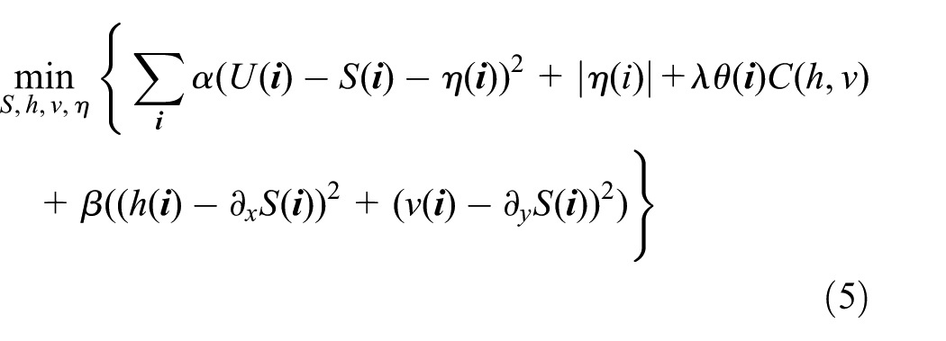
We point out that the map r is proposed by Xu and Jia ³⁴ to preserve salient edges and remove some narrow strips. As analyzed in Xu and Jia, ³⁴ a large value of r indicates that there exist strong image structures in the local window, whereas a small value of r indicates that the area is flat.

Optimization

It is difficult to solve the energy function in equation (3) as it involves a hybrid norm. We use alternating minimization proposed by Wang et al. ¹⁶ to solve in equation (3). By introducing new auxiliary variables $\eta$ , h, and v, we rewrite the energy function equation (3) as

$$\begin{array}{c}\multicolumn{1}{c}{\underset{S,h,v,\eta }{min}\{\sum _{\mathit{i}}\alpha (U(\mathit{i})-S(\mathit{i})-\eta (\mathit{i}){)}^2+|\eta (i)|+\lambda \theta (\mathit{i})C(h,v)}\\ \multicolumn{1}{c}{+\beta ((h(\mathit{i})-{\partial }_{x}S(\mathit{i}{))}^2+(v(\mathit{i})-{\partial }_{y}S(\mathit{i}){)}^2)\}}\end{array}$$

(5)

where $\alpha$ and $\beta$ are positive parameters, and solvers of equation (5) converge to equation (3) when $\alpha$ , $\beta \to \infty$ . The optimization problem (equation (5)) can be divided into four tractable subproblems as follows

$$\underset{S}{\min }\left\{\sum _{\mathit{i}}\alpha {(U(\mathit{i})-S(\mathit{i})-\eta (\mathit{i}))}^2+\beta ((h(\mathit{i})-{\partial }_{x}S(\mathit{i}{))}^2+{(v(\mathit{i})-{\partial }_{y}S(\mathit{i}))}^2)\right\}$$

(6)

$$\underset{\eta }{min}\{\sum _{\mathit{i}}\alpha {(U(\mathit{i})-S(\mathit{i})-\eta (\mathit{i}))}^2+|\eta (\mathit{i})|\}$$

(7)

$$\begin{array}{c}\underset{h}{min}\{\sum _{\mathit{i}}\lambda \theta (\mathit{i})\parallel h{\parallel }_0+\beta {(h(\mathit{i})-{\partial }_{x}S(\mathit{i}))}^2\}\hfill \end{array}$$

(8)

$$\begin{array}{c}\underset{v}{min}\{\sum _{\mathit{i}}\lambda \theta (\mathit{i})\parallel v{\parallel }_0+\beta {(v(\mathit{i})-{\partial }_{y}S(\mathit{i}))}^2\}\hfill \end{array}$$

(9)

Solving S

As equation (6) is a least squares problem, we can obtain its closed-form solution based on the convolution theorem of Fourier transformations. By utilizing the fast Fourier transformation (FFT) to speed up the whole process, the closed-form solution of equation (6) is

$$S={\mathcal{F}}^{-1}\left(\frac{\alpha \mathcal{F}(U)+\alpha \mathcal{F}(\eta )+\beta (\overline{\mathcal{F}({\partial }_x)}\mathcal{F}(h)+\overline{\mathcal{F}({\partial }_y)}\mathcal{F}(v))}{\alpha \mathcal{F}(1)+\beta (\overline{\mathcal{F}({\partial }_x)}\mathcal{F}({\partial }_x)+\overline{\mathcal{F}({\partial }_y)}\mathcal{F}({\partial }_y))}\right)$$

(10)

where $\mathcal{F}(·)$ and ${\mathcal{F}}^{-1}(·)$ denote the FFT and the inverse FFT, and $\overline{\mathcal{F}(·)}$ denotes the complex conjugate of $\mathcal{F}(·)$ .

Solving $\eta$

Given S, we can solve equation (7) by matrix calculus. Similar to Wang et al., ¹⁶ the solver of equation (7) can be given by

$$\eta (i)=\zeta ·\mathrm{sgn}(U(\mathit{i})-S(\mathit{i}))$$

(11)

where $\zeta (\mathit{i})=\max \{|U(i)-S(\mathit{i})|-(1/2\alpha ),0\}$ , $\mathrm{sgn}(·)$ is a sign function, and $\alpha$ is a parameter.

Solving h

Problem (8) can be solved by $L_0$ minimization directly. However, the result is sensitive to noise-like structures. Thus, we introduce an additional pre-smoothing step. To remove small-scale details in ${\partial }_{x}S(\mathit{i})$ , a smooth version of ${\partial }_{x}S(\mathit{i})$ is pre-computed by

$$\widetilde{S_x(\mathit{i})}=\arg \underset{\widetilde{S_x(\mathit{i})}}{min}\{\sum _{\mathit{i}}(\widetilde{S_x(i})-{\partial }_{x}S(\mathit{i}{))}^2+{\chi }_1\parallel \nabla \widetilde{S_x}{\parallel }_0\}$$

(12)

where ${\chi }_1$ is a positive smoothing parameter. equation (12) is a $L_0$ gradient minimization ¹⁵ and easy to solve. It is unnecessary to go into details here. Given $\widetilde{S_x}(i)$ , we rewrite equation (8) and solve h by

$$\begin{array}{c}\underset{h}{min}\{\sum _{\mathit{i}}\beta (h(i)-\widetilde{S_x(\mathit{i}}{))}^2+\lambda \theta (\mathit{i})\parallel h{\parallel }_0\}\hfill \end{array}$$

(13)

The shrinkage formula is utilized to obtain the closed-form solution h, which is given by

$$\begin{array}{c}h(\mathit{i})=\{\begin{array}{cc}\widetilde{S_x(\mathit{i})},\hfill & {(\widetilde{S_x(\mathit{i})})}^2\ge \frac{{\chi }_1\theta (\mathit{i})}{\beta }\hfill \\ \multicolumn{1}{c}{0,}& \mathrm{otherwise}\hfill \end{array}\hfill \end{array}$$

(14)

Solving v

Similarly, a smooth version of ${\partial }_{y}S(\mathit{i})$ can be computed by

$$\widetilde{S_y(\mathit{i})}=\arg \underset{\widetilde{S_y(\mathit{i})}}{min}\{\sum _i{(\widetilde{S_y(\mathit{i})}-{\partial }_{y}S(\mathit{i}))}^2+{\chi }_2\parallel \nabla \widetilde{S_y}{\parallel }_0\}$$

(15)

where ${\chi }_2$ is a positive smoothing parameter. equation (15) is also a $L_0$ gradient minimization ¹⁵ and easy to solve. Given $\widetilde{S_y}(\mathit{i})$ , we rewrite equation (9) and solve v by

$$\begin{array}{c}\underset{v}{min}\{\sum _{\mathit{i}}\lambda \theta (i)\parallel v{\parallel }_0+\beta (v(\mathit{i})-\widetilde{S_y(\mathit{i}}{))}^2\}\hfill \end{array}$$

(16)

The shrinkage formula is utilized to obtain the closed-form solution v, which is given by

$$\begin{array}{c}v(\mathit{i})=\{\begin{array}{cc}\widetilde{S_y(\mathit{i})},\hfill & (\widetilde{S_y(\mathit{i}}{))}^2\ge \frac{{\chi }_2\theta (\mathit{i})}{\beta }\hfill \\ \multicolumn{1}{c}{0,}& \mathrm{otherwise}\hfill \end{array}\hfill \end{array}$$

(17)

Algorithm 1 summarizes the proposed alternating minimization algorithm.

Algorithm 1. Adaptive $L_0$ gradient optimization.
Input: image U, parameters $\lambda$ , $\alpha$ , $\kappa$ and ${\beta }_{\max }$ .
Initialize $S=U$ , ${\beta }_0=\lambda$ , ${\chi }_1={\chi }_2={\beta }_0^2$ , $t=1$ .
while $\beta <{\beta }_{\max }$ do
solve ${\eta }^t$ by equation (11).
solve ${\widetilde{S_x}}^t,{\widetilde{S_y}}^t$ by minimizing equations (12) and (15).
solve $h^t$ and $v^t$ by equations (14) and (17).
solve $S^{t+1}$ by equation (10).
update parameter $\beta \to \kappa \beta$ .
end while
Output: the filtered image S.

Analysis and discussion

In this section, we provide more insights and analysis on how the proposed algorithm performs on image filtering and demonstrate the function of each component of the algorithm separately.

Local weighted function $\theta$

The regularization term usually plays a critical role in the optimization-based filtering methods. In this article, we propose an adaptive regularization, which involves an adaptive function $\theta$ . As mentioned in section “Adaptive $L_0$ gradient minimization model,” $\theta$ relies on another local gradient measurement r, which is used to measure the usefulness of image edges in motion deblurring. ³⁴ By performing thresholding on r, narrow strips and tiny edges can be successfully removed. In the proposed model, we employ $\exp (-\parallel r{\parallel }^{0.8})$ to form an adaptive function $\theta$ . Indeed, $\theta$ works as a structure descriptor and r is a pixel-wise adaptive map. Figure 1 visualizes r and $\theta$ of a synthesized image. The noisy input image shown in Figure 1(a) is roughly piecewise constant and contains several step edges of different magnitudes. Figure 1(b) is the visualization of r, which shows that step edges imply large r. Correspondingly, the adaptive function $\theta$ is small on step edges and large in roughly flat regions, as can be seen in Figure 1(c).

Figure 1.

The visualization of (b) r map and (c) adaptive weight function $\theta$ of the input image (a).

In the proposed method, the adaptive function $\theta$ is capable of removing littery details. To better illustrate the effectiveness of $\theta$ , we show an example in Figure 2. Figure 2(a) is the input image. Figure 2(b) is generated by the proposed method without computing $\theta$ , that is, $\theta (\mathbf{i})=1$ for each pixel. Figure 2(c) is the filtered output of our method. Figure 2(b) contains some small-scale details such as the floor’s texture. It can be seen that our method performs better.

Figure 2.

The function of $\theta$ in removing tiny edges. (a) Input image. (b) Result without computing $\theta$ . (c) Ours with $\theta$ . Here, λ = 0.012, $\kappa =2$ for (b) and (c).

Moreover, we find that $\theta$ also helps to preserve middle-scale structures, as shown in Figure 3. Figure 3(a) is a 1D input signal with both large-scale structures and middle-scale structures. Figure 3(b) is generated by the proposed method without computing $\theta$ . Figure 3(c) is the filtered output of our method. The method without computing $\theta$ loses middle-scale structures. In contrast, our method preserves middle-scale structures adaptively, as shown in Figure 3(c).

Figure 3.

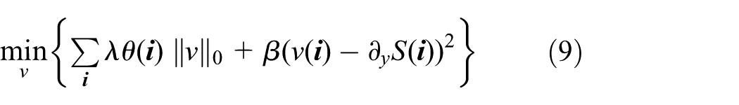
Comparisons of various smoothing methods on a 1D signal. Black curves represent the noisy input; red curves represent the smoothing results. (a) Input noisy 1D signal. (b) Without computing $\theta$ . (c) Ours. For fair comparisons, we set λ = 0.0012, $\kappa =2$ .

The effectiveness of pre-smoothing

In the proposed method, we use $(\widetilde{S_x},\widetilde{S_y})$ instead of $({\partial }_{x}S,{\partial }_{y}S)$ to solve the auxiliary variables $(h,v)$ . We find that this pre-smoothing step is very critical to avoid staircase effect. The efficient iterative algorithm enhances the smoothing ability and reduces the staircase effect. Figure 4 shows that our method can avoid staircase effect. Figure 4(a) is a natural image with analogous texture and inhomogeneous color. Figure 4(b) is generated by the proposed method without pre-smoothing step and Figure 4(c) is the filtered output of our method. Compared with our method, the method without pre-smoothing step generates staircase effect. Our method avoids staircase effect effectively.

Figure 4.

The effectiveness of pre-smoothing. (a) Input image. (b) Result of without pre-smoothing step. (c) Our method. (d)–(f) Close-ups of corresponding images in (a)–(c). Here, $\lambda =0.0015,\kappa =2$ for (b) and (c).

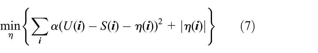
The effectiveness of $L_1$ fidelity term

As mentioned in Shen et al., ³¹ the $L_2$ fidelity term is less effective than $L_1$ fidelity term when the erroneous measurements exist. To verify the effectiveness of the $L_1$ fidelity, we show an example in Figure 5. Figure 5(a) shows a noisy image. Figure 5(b) is generated by $L_2$ fidelity term. Figure 5(c) is generated by the method of Shen et al. ³¹ Figure 5(d) shows the filtered output of our method. As can be seen, our method is effective to removing noise-like structures and generates a much smoother result.

Figure 5.

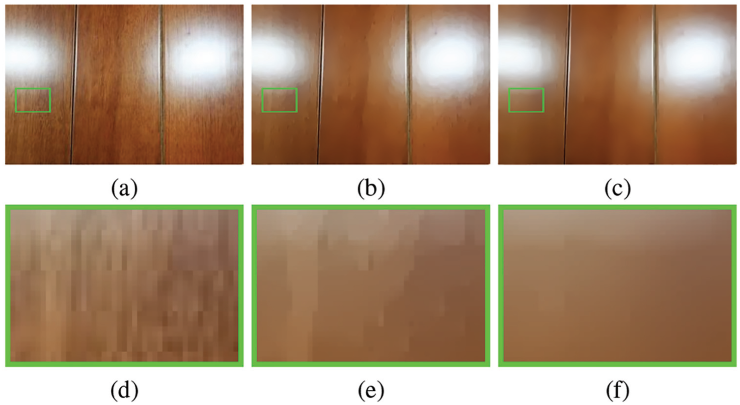
Our method is effective to remove noise-like structures. (a) Input noisy image. (b) The method using $L_2$ fidelity term.(c) The method of Shen et al. ³¹ using $L_1$ fidelity term. (d) Our method with $L_1$ fidelity term. We set $\lambda =0.03$ , $\kappa =2$ for (b)–(d). There are many residual noises in (b) and (c).

Experiments and applications

In this section, we apply the proposed filter to several applications in image editing, including noise removal, clip-art compression artifact removal, detail enhancement and edge extraction, image abstraction and pencil sketching, and HDR tone mapping.

Parameter analysis and settings

We first provide some analysis on the role of parameters. The key parameter $\lambda$ is the weight on the adaptive regularized term, and it is critical to effectively control the level of structure coarseness. Larger $\lambda$ usually results in a more smoothing output. On the contrary, if it is too small, the output image may be very similar to the input image. Figure 6 shows a visual example with results from varying values of $\lambda$ . $\alpha$ and $\beta$ are introduced using alternating minimization technique. As $\alpha$ controls the weight of data term when computing $\eta$ using equation (7), it is not suggested to be too large to avoid over fitting. By contrast, $\beta$ varies during each iteration. It is increasing at the rate of $\kappa$ . $\epsilon$ is the window size when computing the adaptive function $\theta$ . The choice of $\epsilon$ is followed by Xu and Jia. ³⁴ ${\chi }_1$ and ${\chi }_2$ are both introduced for solving h and v. They are regularization parameters in equations (12) and (15) for pre-smoothing on ${\partial }_{x}S$ and ${\partial }_{y}S$ . Thus, it should be set differently for different images.

Figure 6.

Effects of varying $\lambda$ settings on smoothing results of the proposed filter. Larger $\lambda$ leads to smoother output. For fair comparisons, we set $\kappa =2$ for (b)–(e). (a) Input image, (b) λ = 0.001, (c) λ = 0.008, (d) λ = 0.015, and (e) λ = 0.03.

In all experiments, we empirically set ${\beta }_{\max }=100,000$ , $\alpha =1.1$ , $\kappa =2$ , $\epsilon =7$ , ${\beta }_0=\lambda$ , ${\chi }_1={\chi }_2={\beta }_0^2$ . The range of $\lambda$ is $[0.001,0.05]$ . Most computation is spent on FFT in equation (10) and pixel-wise algebraic operations in equations (12), (13), (15), and (16). It takes about 5 s to process a single-channel $600\times 450$ image on an Intel Xeon CPU @ 2.53G with our MATLAB implementation.

Image denoising

As a smoothing image filter, the proposed method can be applied to image denoising. Figure 7 shows an example compared with commonly used image filters including relative total variation (RTV), ³⁵ WLS, ⁸ rolling guidance filter (RGF), ³⁶ and $L_0$ gradient minimization ( $L_0$ ). ¹⁵ Figure 7(a) is a noisy image. It can be seen that results of RTV, WLS, and RGF shown in Figure 7(b)–(d) still contain heavy noises and lose some salient structures. As shown in Figure 7(e), $L_0$ performs better than RTV, RGF, and WLS. However, it also fails to remove all the noises. Compared with these methods, our method generates result with clean structures and without noise residual, as shown in Figure 7(f).

Figure 7.

Comparisons of various smoothing methods on a noisy image. Results shown in (b)–(e) are generated by RTV, ³⁵ WLS, ⁸ RGF, ³⁶ and $L_0$ . ¹⁵ The parameters of relative total variation are $\lambda =0.01$ , $\sigma =3$ , the parameters of WLS are $\lambda =1$ , $\alpha =1.2$ , the parameters of RGF are ${\sigma }_s=3$ , ${\sigma }_r=0.1$ , the parameters of $L_0$ and the proposed method are $\lambda =0.006$ , $\kappa =2$ . (a) Input, (b) RTV, ³⁵ (c) WLS, ⁸ (d) RGF, ³⁶ (e) L₀, ¹⁵ and (f) ours.

Clip-art compression artifact removal

Cartoon-like images are heavily compressed and contain severe compression artifacts. Xu et al. ¹⁵ analyze that it is difficult to generate satisfied output as the compression artifact is highly dependent on edges. The edge-preserving filters can properly deal with this matter and do not require any learning process. As our method is capable of preserving salient edges, the proposed smoothing method is also suitable for clip-art compression artifact removal. We make a comparison with a set of edge-preserving methods, including BF, ⁵ GF, ²⁶ WLS, ⁸ RTV, ³⁵ RGF, ³⁶ and $L_0$ . ¹⁵ As shown in Figure 8(a), the input image contains some acute edges, which are difficult to deal with. Results of BF, WLS, and $L_0$ shown in Figures 8(d) and (f) and 7(i) fail to remove traces of compression. Results of GF, RTV, and RGF ³⁶ shown in Figure 8(e), (g), and (h) blur the edges and lose some salient structures. Our method shown in Figure 8(j) removes the compression artifacts more successfully as compared to other methods.

Figure 8.

Comparisons on compression artifact removal for a cartoon image. (a) Input image. (b) Result of our method. (c)–(j) Close-ups of the input and results of BF, ⁵ GF, ²⁶ WLS, ⁸ RTV, ³⁵ RGF, ³⁶ $L_0$ , ¹⁵ and our method.

Detail enhancement and edge extraction

Detail enhancement is the process of representing details in a magnified way. We briefly introduce the detail enhancement algorithm, ²⁶ which formulates the enhanced image as

$$E=B+\tau D$$

(18)

where B denotes the image base layer, D denotes the image detail layer, $\tau$ is a parameter that controls the magnification, and E denotes the enhanced image. Generally, the base layer B can be generated by edge-preserving filter. A good base layer is very critical to the final enhanced result. If the base layer is not consistent with the input image, the gradient reversal may appear around edges, which is a problem encountered by BF. ⁵ WLS ⁸ is able to avoid gradient reversal safely. However, it is usually time-consuming to compute a five-point spatially inhomogeneous laplacian matrix for WLS.

The proposed method can be applied to detail enhancement based on the decomposition in equation (18). We show an example of detail enhancement in Figure 9. Figure 9(a) is a natural image. Result of BF ⁵ shown in Figure 9(b) displays the gradient reversal artifacts. Figure 9(c) shows the result of $L_0$ gradient minimization. ¹⁵ Compared with $L_0$ gradient minimization, our result contains more rich details and seems vividly as shown in Figure 9(d).

Figure 9.

Detail enhancement. The parameters of BF are ${\sigma }_s=10$ , ${\sigma }_r=0.2$ . We set $\lambda =0.001,\kappa =2$ for (b) and (c). For (b)–(d), we set $\tau =5$ . (a) Input, (b) BF, ⁵ (c) L₀, ¹⁵ and (d) ours.

Edge extraction is a basic pre-processor of natural image editing and high-level structure inference. It is also a challenging problem because most edge detectors are sensitive to complex structures and unavoidable noises. As analyzed in section “Local weighted function $\theta$ ,” the proposed method is capable of suppressing low-amplitude details and preserving the significative structures. An example is shown in Figure 10. Figure 10(a) is a challenging input image and its gradient map is shown in Figure 10(d). Figure 10(g) is the edge extraction result of Figure 10(d) by canny edge detector. Figure 10(b) and (c) shows the corresponding results of $L_0$ gradient minimization ¹⁵ and the proposed method. Figure 10(e) and (f) shows the corresponding gradient maps of Figure 10(b) and (c) with linear enhancement for visualization. Figure 10(h) and (i) shows the corresponding edge maps of Figure 10(b) and (c). Compared with $L_0$ gradient minimization, ¹⁵ the proposed method preserves most significant structures (such as the woman’s shirt and the boundary of clouds), and the filtered output is more reliable.

Figure 10.

Edge enhancement and extraction. The parameters are $\lambda =0.045,\kappa =2$ for (b) and (c). Our method suppresses low-amplitude details and preserves high contrast edges. (a) Input, (b) L₀, ¹⁵ (c) ours, (d) gradient map of (a), (e) gradient map of (b), (f) gradient map of (c), (g) edge map of (a), (h) edge map of (b), and (i) edge map of (c).

Image abstraction and pencil sketching

Usually, the visual perception of an image can be enriched with textures and details. In some cases, we prefer simplified stylistic pictures which are non-photorealistic abstraction with suppressing details and emphasizing edges from color images or videos. Conventional image abstraction methods contain two main steps—image smoothing step and edge component detecting step. To increase the visual distinctiveness of different regions, the extracted lines are added back to the smoothed image. Based on the video abstraction framework of Winnemöller et al., ²² we apply the proposed method to image abstraction task. Figure 11 shows an example. The result of $L_0$ gradient minimization ¹⁵ is shown in Figure 11(b). Our method performs better than Xu et al. ¹⁵ We also show pencil sketching results of Figure 11(a)–(c) in Figure 11(d)–(f). As can be seen, our pencil sketching result shown in Figure 11(f) contains more details than that of Xu et al. ¹⁵

Figure 11.

Image abstraction and pencil sketching results. For fair comparisons, we set the parameters λ = 0.003, $\kappa =2$ for (b) and (c). Our method removes the least important structures and generates a more hierarchical result. (a) Input, (b) L₀, ¹⁵ (c) ours, (d) pencil stylization of (a), (e) pencil stylization of (b), and (f) pencil stylization of (c).

HDR tone mapping

HDR mapping is another popular image editing task which aims to generate low dynamic range images by compressing the base layer to some level. The base layer should be smooth enough to generate reasonable contrast maintenance in range compression. Within the tone mapping framework of Durand and Dorsey, ⁶ the proposed filter can be used to generate the base layer. We show a tone mapping example in Figure 12 and compare it with some other commonly used methods. We first convert the input HDR radiance to a logarithmic scale (log10). Then we map the result to $[0,1]$ and display it in Figure 12(a). The result of WLS ⁸ shown in Figure 11(b) contains some dark regions. A blocky reflection also appears on the floor. The result of $L_0$ ¹⁵ is shown in Figure 12(c). As can be seen, our method shown in Figure 12(d) contains more details than Figure 12(b) and (c).

Figure 12.

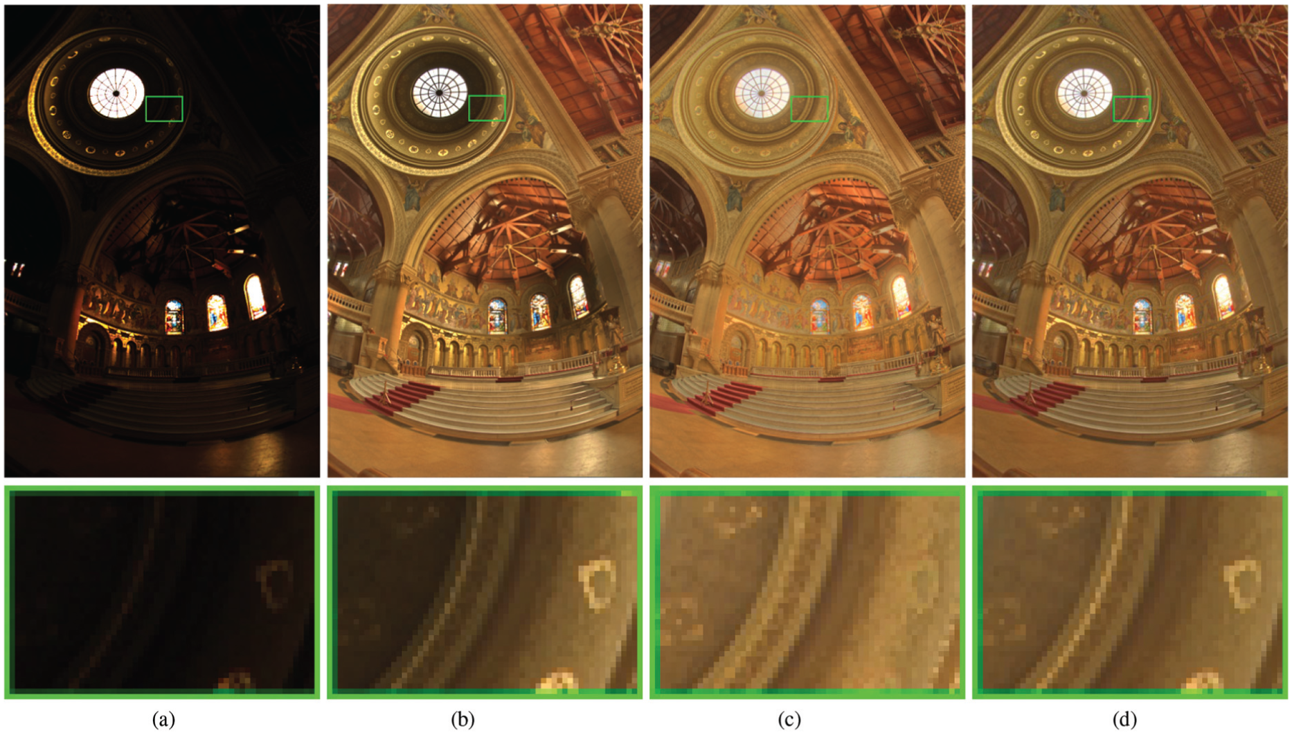
Comparisons of HDR tone mapping using different methods. Top row: results by several different filtering methods. Bottom row are close-ups of corresponding images in the top row. The parameters of WLS are $\lambda =20$ , $\alpha =1.2$ . We set the parameters λ = 0.003, $\kappa =2$ for both (c) and (d) for fair comparison. (a) Input, (b) WLS, ⁸ (c) L₀, ¹⁵ and (d) ours.

Conclusion

In this article, to enrich the image processing technology of WMSNs images, we present an adaptive image filter based on $L_0$ gradient minimization framework. We utilize an adaptive function to facilitate detail removal and preservation of salient edges. We also develop an efficient iterative algorithm to solve the proposed model. The proposed filter behaves robustly to noise and avoids staircase effect effectively. Experimental results on several computer vision tasks show that the proposed method performs favorably against the state-of-the-art filtering methods. It is also appreciated to extend our method to more applications.

Our method is adaptive to preserve middle-scale details and remove small-scale details without employing prior texture information. If the structures and textures of the image are visually similar in scales, it is hard to distinguish between structures and textures; thus, part of the structures can be easily mistaken as textures. As can be seen from Figure 13, Figure 13(a) is a input image with scale and appearance similar to the underlying textures. Since the input image contains textures with strong contrast and the underlying textures are exceedingly too close to the scale and shape of these edges, the visually filtering output of our method is shown in Figure 13(b). As can be seen, our method is failed to preserve all of the structures.

Figure 13.

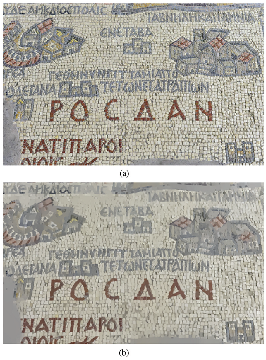
Difficult examples. Our method is failed to extract structures whose scale and appearance are similar to the textures. We set the parameters λ = 0.0015, $\kappa =2$ . (a) Input and (b) ours.