Sage Journals: Discover world-class research

Abstract

Nowadays, smartphones are widely and frequently used in people’s daily lives for their powerful functions, which generate an enormous amount of data accordingly. The large volume and various types of data make it possible to accurately identify people’s travel behaviors, that is, transportation mode detection. Using the transportation mode detection, results can increase commuting efficiency and optimize metropolitan transportation planning. Although much work has been done on transportation mode detection problem, the accuracy is not sufficient. In this article, an accurate traffic pattern detection algorithm based on multimodal sensing is proposed. This algorithm first extracts various sensory features and semantic features from four types of sensor (i.e. accelerator, gyroscope, magnetometer, and barometer). These sensors are commonly embedded in commodity smartphones. All the extracted features are then fed into a convolutional neural network to infer traffic patterns. Extensive experimental results show that the proposed scheme can identify four transportation patterns with 94.18% accuracy.

Keywords

Deep learning low power consumption transportation mode detection multimodal sensing performance comparison

Introduction

Transportation mode detection (TMD) is considered as a special activity recognition, which aims to automatically identify the transportation modes of persons.¹ Accurately capturing and analyzing the individual commuting behavior patterns produces positive impacts on many aspects of human life. Accurate monitoring of human transportation behaviors not only helps track human mobility and optimize the transportation mode selection, but also can facilitate urban transportation planning and health monitoring.

Much research has been conducted on TMD based on GPS (Global Positioning System), geographic information systems (GIS), and light-weight sensors. While GPS-based TMD methods can identify transportation patterns with high accuracy when GPS signals are available in the outdoor open environment, these methods suffer from high power consumption and failure in indoor/underground spaces and urban canyons where the GPS signals are shielded.² Furthermore, GPS-based solutions provide only modest accuracy which cannot support a fine-grained distinction of motorized transportation modes. To enhance the accuracy of TMD, other work utilized the real-time locations and trajectories of transportation tools from GIS (Geographic Signal System). The availability of this method is strictly limited due to high power consumption and background support. Recently, light-weight sensors–based traffic pattern recognition methods attract much attention.³ It utilizes the accelerator to sense the characteristic of various transportation modes with low power consumption. This method can work well without the need of infrastructure support. However, it is challenging to cope with complex noise produced by various road flatness and driver styles.

Numerous studies have confirmed that the deep learning model, formed by stacking several layers of shallow structures, have excellent features representation capability, and could effectively tackle nonlinear and complex classification problems. Our previous work adopted deep learning to solve the transportation mode recognition problem⁴ and achieved reasonable results. However, this approach is still at an initial stage and need further investigation to improve the accuracy and generalization for heterogeneous devices which integrate different numbers and types of sensors.

In this article, a novel traffic pattern detection algorithm based on multimodal sensing was proposed. By introducing several semantic and sensory features and constructing individual classifiers for each type of sensors, 94% accuracy is obtained with better adaptability for heterogeneous devices, that is, the proposed algorithm still works well if a sensor, for example, barometric sensor, is not integrated in a mobile phone.

The main contributions of this article are summarized as follows:

Introducing several semantic features (i.e. turning and pause frequencies) and additional sensory features (barometer) to improve the accuracy of detecting transportation pattern. These features are closely related to the specific transportation pattern as a whole and help to differentiate various transportation modes. For example, the turning frequency feature can effectively identify the car and the bus due to the complex environment of the urban canyon and the urban roads with dense crossroads. When different kinds of vehicles run on these roads, they demonstrate remarkably different turning frequencies. Besides, the train and the metro are also distinctive in turning frequency characteristic. On the city roads with heavy traffic, these four kinds of vehicles present different pause characteristics. The pause frequency and the rest time are two prominent features, which have good distinctiveness.

Constructing individual convolutional neural network (CNN) for each type of sensors to handle the heterogeneity of devices integrating different numbers and types of sensors. When the barometric sensor is not integrated in a certain mobile phone, the proposed algorithm can still identify the vehicles with high accuracy.

The rest of this article is organized as follows. Section “Related work” introduces the related work. Section “Transportation pattern detection” describes the proposed transportation pattern detection method, including the algorithm architecture, feature extraction, and system architecture. Section “Evaluation and analysis” shows the experimental results and analysis, and section “Conclusion” summarizes the conclusion.

Related work

The idea to use smartphones for monitoring transportation behavior in this article has been widely discussed. Previous work mainly focused on the different characteristics obtained from various sensors embedded in smartphones or the combination of them. The sources of these features have a critical influence on the performance of traffic pattern recognition. Introducing complementary sensors as data source can improve the transportation recognition accuracy. The original data used for detecting transportation modes can be classified into the following two main types: (1) external sources, which rely on the infrastructures, such as GPS satellites, WiFi routers, and GSM (Global System For Mobile Communications) base stations. The availability of external sources are limited. (2) Internal sources, which are obtained from the sensors embedded in smartphones. They provide stable data sources. Table 1 lists some representative work on transportation recognition using different data sources.

Table 1.

Data sources used by the existing transportation recognition methods.

Paper	External source				Internal source
Paper	GPS	GIS	GSM	WiFi	Accelerometer	Magnetic	Gyroscope	Barometer	Platform
This article					√	√	√	√
Using mobile phones to determine transportation modes⁵	√				√
Transport mode detection with realistic Smartphone sensor data⁶	√				√
Using smartphones for transportation mode classification⁷			√		√
Using GPS-derived speed patterns for recognition of transport modes in adults⁸	√
Understanding transportation modes based on GPS data for web applications⁹	√
Classifying spatial trajectories using representation learning¹⁰	√
Detecting transportation modes using deep neural network¹¹	√								√
Accelerometer-based transportation mode detection on smartphones¹²					√
Toward indoor transportation mode detection using mobile sensing¹³				√	√
Travel mode identification with smartphones¹⁴					√	√	√	√
Transportation mode detection using mobile phones and GIS information¹⁵	√	√
Transportation behavior sensing using smartphones¹⁶	√				√
Transportation mode recognition algorithm based on Bayesian voting¹⁷			√		√	√	√	√
Use of acceleration data for transportation mode prediction¹⁸					√

GIS: geographic information systems; GPS: global positioning system; GSM: global system for mobile communications.

External sources such as GPS, GIS, and GSM are widely used in transportation mode identification. Abundant features such as geographical coordinates, travel velocity, acceleration make GPS a good option for TMD. Endo et al.¹⁰ take only GPS data as data source and achieve a moderate accuracy. GIS is another expressive data source, which can be used to assist GPS-based transportation recognition using the real-time spatial data. For a sample, Stenneth et al.¹⁵ extracted GIS data including the real-time bus locations, spatial rail, and spatial bus stop information and achieved 17% accuracy improvement. GSM provides a coarse network-based location, which can also be used for transportation recognition similar to the function of GPS.

D Shin et al.⁷ use the coarse network location and accelerometer data to build the transportation pattern classifier. On the whole, external sources have many constraints. The GPS-based transportation recognition method consumes considerable power and cannot work effectively when GPS signal is obstructed. The GIS-based method is limited when the location is not updated timely.

The internal sources used for transportation mode recognition include accelerometer, gyroscope, field magnetic, and barometer which are embedded in many commodity smartphones. Since the acceleration patterns of different transportation tools are distinctive, accelerometer appears in almost every TMD model. For example, the acceleration variation of a pedestrian walking is much larger than motorized vehicle.⁸ S Hemminki et al.¹² proposed a classifier model based on accelerometer data, in which decision trees and Adaboost classifier are applied as sub-classifier. The atmosphere pressure is also used for transportation mode recognition. The pressure fluctuates more greatly in a metro than in a car or bus. Su et al.¹⁴ explain that the pressure variances are caused by the trunk structure and the surrounding environment.

In general, the TMD accuracy using a single sensor is usually limited and dramatically influenced by the heterogeneity of smartphones. To improve accuracy, multiple sensors are leveraged. Reddy et al.⁵ introduced the accelerometer into the GPS-based method and achieved better accuracy compared with the GPS-based method. Hemminki¹⁶ achieved 93.6% accuracy by combining the GPS and the accelerometer. As comparison, if only the accelerometer data are used, the transportation recognition accuracy decreases by 10.4%. If only the GPS data are used, the transportation recognition accuracy decreases by 19.2%. Thus, the combination of using more sensors can improve the performance of transportation mode recognition.

Many classification methods have been applied in transportation mode recognition such as Naïve Bayes (NB),^5,14,15,19 support vector machine (SVM),^5,11,20,21 adaptive boosting (Adaboost),¹⁵ decision tree (DT),^2,21 random forest (RF),^14,15,18 multilayer perception (MLP),^15,19 K-nearest neighbor (KNN),²⁰ continuous hidden Markov model (CHMM),^5,20 and discrete hidden Markov model (DHMM).²⁰ However, these methods could not effectively extract the deep feature of human behavior and optimize the performance through parameter adjustment.

In recent years, deep learning methods are adopted for TMD.^2,4,11 By extracting deep features from a set of hand-crafted features, these methods achieved reasonable accuracy. Gong et al.⁴ used CNN algorithm to sense transportation with 169 hand-crafted features and achieved high transportation recognition accuracy. Considering that all the sensor data are combined together to feed the CNN model, its adaptability to heterogeneous smartphones integrating with different number and types of sensors is limited. To improve adaptability to device heterogeneity, this article proposed multiple CNN–based transportation recognition algorithm. Each CNN model is built for an individual sensor, which is fit for different numbers and types of sensors.

Deep feature extraction from raw data is an important character of deep neural network applications. Y Endo et al.¹⁰ and Y Bengio et al.²² introduce how to automatically extract features using the deep neural network from the trajectory images and how to use a neural network for data dimension reduction.

Transportation pattern detection

System architecture

The architecture of the proposed transportation recognition system is depicted in Figure 1. The mobile phones are equipped with a variety of sensors to collect data in the bottom layer. After collecting data, the features of each sensor are extracted. The features are described in section “Feature extraction”; afterward, the extracted features are fed into the four CNN models to recognize the pattern (model will be presented in sections “Accelerometer feature” and “Gyroscope, geomagnetic, and barometric”). Each CNN outputs an intermediate result. The final result is determined by voting all the intermediate results.

Figure 1.

The architecture of the proposed transportation recognition system.

Data preprocessing and feature extraction

Data pretreatment

The raw data is collected from the sensors in the smartphones. Before analyzing the data and extracting useful features, the raw data are preprocessed to remove jitter. Accordingly, the paper proposes the method for estimating the gravity component from accelerometer measurements that improve the robustness of gravity estimation, particularly in the presence of sustained acceleration.

The data preprocessing includes two stages. First, to mitigate the variation of the data, the original data are imported to a low-pass filter and the data are equalized by a sliding window of 1.2 s and 50% overlap. Second, horizontal acceleration is extracted from the original data and the gravity estimation is realized accordingly.

Gravity estimation

The coordinate system of mobile phones for data collection is shown in Figure 2. The original data are collected based on the mobile phone coordinate system. When a wearer moves, the three-axis accelerometer configuration is in some arbitrary orientation on the wearer’s body. In order to accurately recognize transportation pattern, the linear acceleration information without gravity component in terms of a global reference coordinate, is useful to identify vehicles. Once the measurements have been obtained, the sensor measurements are projected to this global reference frame by estimating the gravity component along each axis and calculating gravity eliminated projections of vertical and horizontal acceleration.

Figure 2.

Relevant coordinate systems of mobile phone systems.

Currently, the main method for gravity estimation from accelerometer sensor is to calculate the mean over a sliding window within a fixed duration.²³ The accuracy of gravity estimation using this method decreases when a sudden change of movement happens. To decrease the errors caused by the sudden change of movement and the delay of obtaining an accurate gravity estimation when using the aforementioned method, a scheme with variable sliding window is employed to calculate the mean of accelerometer measurements as the gravity component estimation,¹¹ as shown in Figure 3. Considering that the gravity component is oriented to the Earth core, it is used as one axis of the navigation coordinate system. The navigation coordinate system is independent on the mobile phone coordinate system and can be used as the standard basis for accurate estimation of transportation pattern to eliminate the influence of arbitrary mobile phone poses.

Figure 3.

Eliminate gravity.

The main steps to estimate gravity component using a variable sliding window are denoted as follows:

A sample of five frames is taken as a big window for gravity estimation;

A new sample is composed of new data and historical data when window is sliding;

Firstly, the mean(w₁) and variance(w₂) value of a samples are calculated;

If there is a great differences (more than 4 m/s²) between average acceleration in a sliding window and estimated gravity acceleration (the average value of the large window), variance threshold will reset;

Then if the variance of the new sample in sliding windows is relatively small (not more than 1.5xl), program flow will do step (6), otherwise the program flow will do step (9);

Next, if the variance of the new sample in sliding windows is less than the gravity acceleration variance threshold (1 m/s²), program flow will do step (7), otherwise the program flow will do step (8).

The mean value of the acceleration in the sliding window evaluates the estimated gravity acceleration. In the sliding window, the mean value of acceleration variance and gravity acceleration variance threshold are conducted as a new dynamic variance threshold, which are used to reduce the variance threshold dynamically, and update the variance increment parameter at the same time. The algorithm is over;

According to the variance increment parameter, the gravity acceleration variance threshold is increased. This algorithm is over;

If it is considered to be the continuous acceleration and deceleration phase, the average value of the small window will no longer used to estimate the gravity acceleration. The average value of the large window is taken as the estimated gravity acceleration. The algorithm is over.

Horizontal acceleration

The vertical acceleration vector v is estimated corresponding to gravity as v = (v_x, v_y, v_z), where v_x, v_y, and v_z are averages of all the measurements on those respective axes for the sampling interval.

Let $a (a_{x}, a_{y}, a_{z})$ be a frame of a triaxial accelerometer. And $d = (a_{x} - v_{x}, a_{y} - v_{y}, a_{z} - v_{z})$ to represent the dynamic component of a. So p is the vector of the acceleration in the direction of gravity in formula (1), and h, horizontal acceleration, is calculated by formula (2)²³

p = (\frac{d • v}{v • v}) v

(1)

h = d - p

(2)

By preprocessing the raw data, some data jitter and noise are eliminated. The influence of gravity on extraction features is eliminated. A good prerequisite for extraction features is provided after the raw data is preprocessed.

Feature extraction

As we all know, one of the most important things in pattern recognition is to find the best features that can distinguish different categories. In order to make full use of the raw data, it is necessary to explore the features on each sensor. These characteristics can play a positive role in distinguishing all kinds of transportation patterns. Next these characteristics will be introduced from each sensor measurement in detail. These features are extracted using a sliding window with 256 samples and 50% samples are repeated with the last data window to calculate the features for each time. This method can make use of historical observation and obtain denser feature data, which can improve transportation identification accuracy and real-time performance. Acceleration, gyroscope, geomagnetic, and pressure are extracted separately.

Acceleration features

The data collected by the acceleration should be preprocessed prior to the extraction operation of features. The acceleration features include three types: frame features, peak features, and segment features. Peak features and segment features reflect the mobility mode of the vehicle, rather than the users’ mobile mode. Therefore, peak features and segment features are not sensitive to the position where the user carries the smartphone (inside the pocket or holding in hand). The frame features include statistical features, time domain features, and frequency domain features. Table 2 shows all the characteristics of acceleration.

Table 2.

Acceleration features used for transportation recognition.

Domain	Features
Statistical	Mean; STD; variance; median; min; max; range; interquartile; range; kurtosis; skewness; RMS
Time	Integral; double integral; autocorrelation; mean-crossing rate
Frequency	FFT DC,1,2,3,4,5,6 Hz; spectral energy; spectral entropy; spectrum peak position; wavelet entropy; wavelet magnitude
Peak	Volume (Auc); intensity; length; kurtosis; skewness
Segment	Variance of peak features (10 features); peak frequency (2 features); stationary duration; stationary frequency

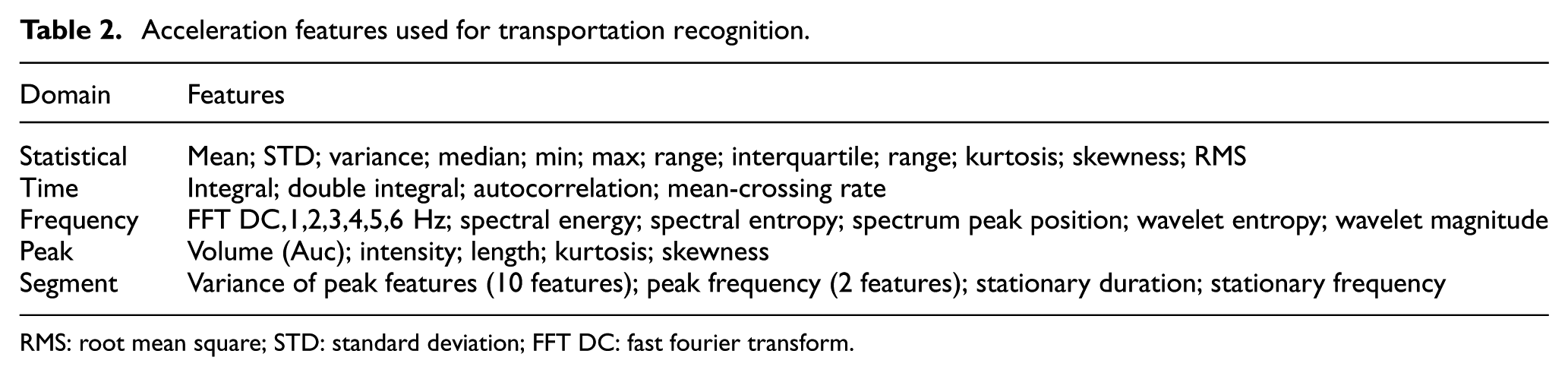
RMS: root mean square; STD: standard deviation; FFT DC: fast fourier transform.

There are some features which need to be further explained in Table 2.

Kurtosis: Represents the flat or abrupt level of the sample probability distribution peak. The kurtosis of the normal distribution is equal to 3, so when the distribution of the data samples is steep than the normal distribution, the kurtosis is greater than 0 (the peak). When the distribution of data samples is flat, the kurtosis is less than 0 (the peak).

Skewness: Represents the symmetry of the distribution pattern of data samples. If the distribution of the sample data is the same as that of the normal distribution, that is, when the mean is equal to the median, the skewness value is 0. When the mean is greater than the median, the skewness is greater than 0; when the average is less than the median, the skewness is less than 0.

Root mean square (RMS): The RMS value of a set of values (or a continuous-time waveform) is the square root of the arithmetic mean of the squares of the values, or the square of the function that defines the continuous waveform. In physics, the RMS current is the “value of the direct current that dissipates power in a resistor.”

Autocorrelation: Autocorrelation is used to describe the interdependencies between values of a sequence at different times.

Spectrum energy: Spectral energy describes the distribution of energy at each frequency point.

Spectral entropy: Entropy represents the degree of uncertainty of the system in information theory, and spectral entropy describes the degree of uncertainty in the amplitude distribution of the source.

Wavelet entropy: Wavelet is defined as a function of finite interval and the average value is zero. Wavelet entropy represents the entropy of energy distribution of each scale of the wavelet.

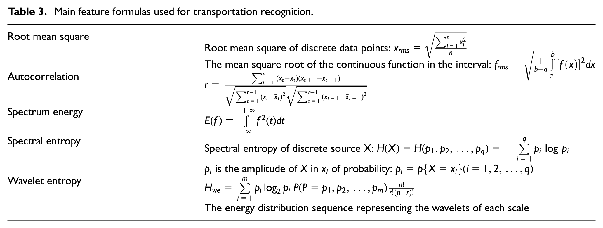
Table 3 lists the definition of partial features.

Table 3.

Main feature formulas used for transportation recognition.

Root mean square	Root mean square of discrete data points: $x_{rms} = \sqrt{\frac{\sum_{i = 1}^{n} x_{i}^{2}}{n}}$ The mean square root of the continuous function in the interval: $f_{rms} = \sqrt{\frac{1}{b - a} \int_{a}^{b} {[f (x)]}^{2} dx}$
Autocorrelation	$r = \frac{\sum_{t = 1}^{n - 1} (x_{t} - {\bar{x}}_{t}) (x_{t + 1} - {\bar{x}}_{t + 1})}{\sqrt{\sum_{t = 1}^{n - 1} {(x_{t} - {\bar{x}}_{t})}^{2}} \sqrt{\sum_{t = 1}^{n - 1} {(x_{t + 1} - {\bar{x}}_{t + 1})}^{2}}}$
Spectrum energy	$E (f) = \int_{- \infty}^{+ \infty} f^{2} (t) dt$
Spectral entropy	Spectral entropy of discrete source X: $H (X) = H (p_{1}, p_{2}, \dots, p_{q}) = - \sum_{i = 1}^{q} p_{i} \log p_{i}$ $p_{i}$ is the amplitude of X in $x_{i}$ of probability: $p_{i} = p {X = x_{i}} (i = 1, 2, \dots, q)$
Wavelet entropy	$H_{we} = \sum_{i = 1}^{m} p_{i} \log_{2} p_{i}$ $P (P = p_{1}, p_{2}, \dots, p_{m}) \frac{n!}{r! (n - r)!}$ The energy distribution sequence representing the wavelets of each scale

Geomagnetic features

The geomagnetic features leverage the distorted Earth’s magnetic fields caused by a vehicle’s mechanical motions. These distorted fields are usually below 50 Hz and can be captured by a Hall-effect sensor, which is popularly integrated in almost all commodity smartphones.

The different speeds of diverse types of vehicles produce remarkable variance of geomagnetic peaks. For example, the high-speed rail is faster than other vehicles, and then it could go through more geomagnetic peaks within a fixed period. This characteristic is beneficial for distinguishing various transportations.

The magnetic variance features of four different vehicles are compared in Figure 4. The geomagnetic variances are calculated with a sliding window (256 samples). The remarkable differences among car, metro, and bus confirm the validity of using the geomagnetic feature to differentiate transportation patterns.

Figure 4.

The variance of magnetic data frame for different transportation tools.

Using the same size of sliding window (256 samples), the following features are calculated including mean, deviation, variance, median, minimum, maximum, range, interquartile range, kurtosis, skewness, RMS, integral, autocorrelation, mean-crossing rate. Figures 5 –7 show RMS/autocorrelation/mean-crossing rate features, respectively.

Figure 5.

The RMS of magnetic data frame for different transportation tools.

Figure 6.

The autocorrelation of magnetic data frame for different transportation tools.

Figure 7.

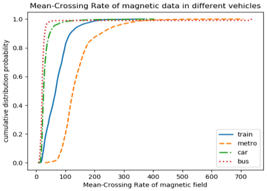
The mean-crossing rate of magnetic data frame for different transportation tools.

Pressure features

Pressure features are an important role for metro. People can feel that there are obvious changes in pressure when people travel by vehicles to different places. Therefore, features are extracted from the data that are collected by a pressure sensor in order to recognize the vehicles. The features are shown in Table 4.

Table 4.

Press features used for transportation recognition.

	Features
Statistical	Mean, STD, variance, median, min, max, range, interquartile range kurtosis, newness, RMS
Time domain	Integral, double integral, autocorrelation, mean-crossing rate
Frequency domain	FFT DC,1,2,3,4,5,6 Hz

RMS: root mean square; STD: standard deviation; FFT DC: fast fourier transform.

Static detection

There is a possibility that transportation tools are in a static state during their movements. The values of sensors are same in this case. Static state detection is regarded as an important step. Tests prove that the classification accuracy can be increased by 2%. Static frequency and duration are two effective features to distinguish the category of vehicles in the process of static detection, which are especially valid in the classification of the car and the bus.

In the process of static detection, if the variance and RMS value of the horizontal acceleration are less than the pre-defined threshold, this situation will be considered as a static state. The threshold is set to 0.1.

Then static frequency and rest time can be obtained from static detection. Static frequency and rest time are put into the classifier for training. After the test, the precision can be increased by 5%–10%.

Turning detection

The turning detection uses the gyroscope sensor data. The data are mapped in the direction of gravity when the angle changes in a corner. The increase of the radian system is compared with the threshold value to obtain the determination results, as shown in formula (3)

\begin{matrix} angle = angle \\ + \frac{gy r_{x} \times gravit y_{x} + gy r_{y} \times gravit y_{y} + gy r_{z} \times gravit y_{z}}{\sqrt{{gravity}_{x}^{2} + {gravity}_{y}^{2} + {gravity}_{z}^{2}}} \end{matrix}

(3)

In formula (3), $gy r_{x}$ , $gy r_{y}$ , and $gy r_{z}$ are representing the component of the gyroscope. $gravit y_{x}$ , $gravit y_{y}$ , and $gravit y_{z}$ represent the component of the gravitational acceleration.

There are many misoperations when people hold the phone, such as a sudden rotation of mobile phones. Misoperations have a great influence on the frequency of turning. So these misoperations are important to identify and remove in an efficient way. In these four types of transportation (car, bus, train, metro), cars are the maximum number of turns, and a single turn takes 2 min at least. So if there is an angle greater than 60 in a single frame (1.28 s), it is judged to be a misoperation.

If a train rounds a corner, it will take longer time than a car or a bus. So a big turn and a small turn should define in this situation. Then we calculate the radian value in 20 frames. And then convert the arc to an angle. A sliding window is used to define a large window and a small window. When the angle in the large window is greater than 50°, the angle should be placed into a small window. This angle value is calculated by a small window slide. If the small window slide is found only an angle value greater than 50°, it is considered there is only a big turn in this window. Otherwise, if you find two, it is considered there are two small turns.

Through deep mining of the characteristics of each sensor, the characteristics of traffic pattern recognition increase a lot of constructive features on the basis of the original data. These features have played an important role in pattern recognition, which make the recognition process become more effective and improving the accuracy.

The CNN architecture algorithm

The method based on deep learning is implemented with Keras,²⁴ which is a flexible, extensible machine learning framework built on TensorFlow.²² Features are extracted from four kinds of mobile sensors.

The evaluation of this model is improved, using different training sets and validation sets. Some previous researches shuffled data set and then separated these data into 80% as training data and 20% as validation data. One problem is that data collected in one file are similar. Thus, the features extracted are similar as well. This results in similar training and test data set. Therefore, evaluation using this data set cannot reveal the generalizability and robustness of the model. We tested the method in Gong et al. with the same data set, and the accuracy rate is 79%.⁴ This model is trained and tested in different data sets.

In this article, two caveats are worth making. (1) The training set and testing set are separately collected. (2) Each sensor has an available classifier. In this way, sensors do not interfere with each other. Each classifier has different network structures and parameters. The improvement of each classifier contributes to the overall system performance. (3) Finally, the final result is voted by all classifiers.

The neural network structure and parameter of each classifier are elaborated as follows.

Accelerometer feature

This method calculated 121 features from accelerometer data in Figure 8:

1. The normalization and reshaping of data: [x₁…x₁₂₁] denotes acceleration feature set. Input features are normalized to a value between [0, 1] by

X_{norm} = \frac{x - min}{max {x} - min {x}}

(4)

where max{x} and min{x} are the maximum and minimum of each column, respectively. After normalization, data are reshaped into an 11 × 11 square matrix.

The advantage of data normalization is that it can quicken the learning speed of the network and improve the predicting precision.

2. A convolution layer: The convolution layer can eliminate noise and improve the training rate efficiency. The output of the jth feature map on the ith unit of the l convolution layer is:

x_{i}^{l, j} = σ (b_{j} + \sum_{a = 1}^{m} w_{a}^{j} x_{i + a - 1}^{l - 1, j})

(5)

where $b_{j}$ is the bias term for the jth feature map. m is the kernel size. $w_{a}^{j}$ is the weight of jth feature map and ath filter index. $σ$ is the activation function which is ReLu. The kernel size is (3 × 3).

3. A pooling layer: The average pooling layer size is 2 × 2. The average pooling process based on equation (6)

x_{i}^{l, j} = max_{n \in [1, r]} x_{(i - 1) \times T + n}^{l - 1, j}

(6)

where n is the pool size and T is the pooling stride. The benefit of max pooling layer is that it reduces the output dimension and sensitivity with a conservation of feature size.

4. A dropout layer: This layer drops certain percent of nodes in the network stochastically. A node is “dropped” because it will not update this time but will be resuscitated in the next round. Dropout layer prevents the model from over-fitting when the training sample is not sufficient enough. The dropout layer diminishes the number of training parameters and the generalization deviation.

5. A fully connected layer: The input of this layer will be mapped to a hidden feature space. The connected layer learns the local features extracted by lower network layers. Finally, the traffic patterns are recognised by a Softmax classifier in equation (7)

f (x) = \arg max_{c} \frac{e^{x^{l - 1} ω_{j}}}{\sum_{n = 1}^{N} e^{x^{l - 1} ω_{n}}}

(7)

where c is the class label, x is the sample feature, l is the layer index, and N is the number of classes.

6. Forward propagation transmits input information to the output layer through the hidden layer, outputs the classification results. The error loss is calculated with equation (8)

L (y) = - \frac{1}{n} \sum_{x} [y \ln a + (1 - y) \ln (1 - a)]

(8)

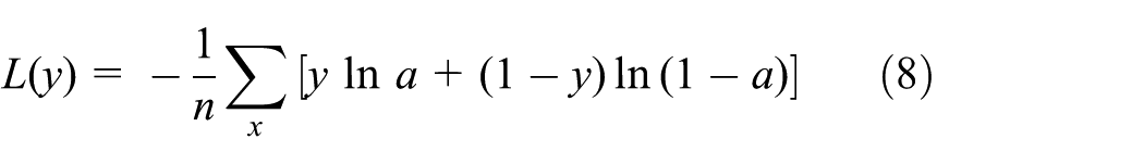
where x is sampled, n is the number of training samples, parameter a is the prediction output, and y is the ground truth.

7. Model evaluation: Normalized and reshaped validation data are input into the network and output corresponding predictions which are compared to the ground truth, and thus, model accuracy is computed.

Figure 8.

The CNN classifier architecture of transportation recognition for the accelerator.

Gyroscope, geomagnetic, and barometric

Training phase

As shown in Figure 9, [x₁₂₁…x₁₄₆] are the 25 features of the gyroscope. Next, these features are normalized by equation (4) and then processed by the connected layer. For the small size of these features, which are not fit for the process of convolution and pooling procedure. Finally, the model files are created by the Softmax classifier.

Figure 9.

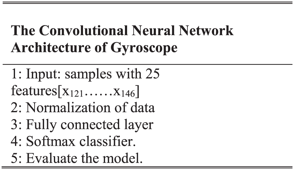
The CNN classifier architecture of transportation recognition for the gyroscope.

Test phase

The test data set will be processed in a similar ways as training phase. Note that the model file generated by the training phase is imported to the classifier for classification, and the final accuracy is voted by four sensors.

Structure of the original data

TMD contain a variety of network architectures. This experiment is based on raw data in deep learning neural network structure. The purpose is to compare which accuracy is higher using with raw data and feature data.

This new frame structure is shown in Figure 10 which can get highest accuracy by using original data.

Figure 10.

The classifier architecture of transportation recognition using the original sensor data.

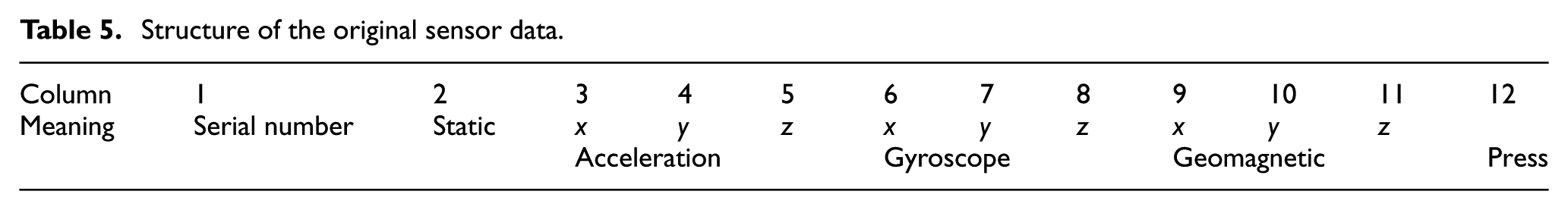
Data preprocessing. The original data includs 12 columns data that is shown in Table 5. It will process these data using a sliding window. The sliding window size is 256. So the data are sampled by a sliding window.

Table 5.

Structure of the original sensor data.

Column	1	2	3	4	5	6	7	8	9	10	11	12
Meaning	Serial number	Static	x	y	z	x	y	z	x	y	z
			Acceleration			Gyroscope			Geomagnetic			Press

Training phase

The basic idea of the model is to use convolutional layers to extract deep features. Through a series of explorations and attempts, the optimal network structure is shown in Figure 10. In order to make full use of collected data, a neural network is built with 10 input which is sequential data from x-, y-, and z-axis of the accelerometer, gyroscope, magnetic sensors, and press sensor. Firstly, the input layer is the first line of Figure 10. After input layer, two convolution layers and two max pooling layers are laid on top of the 10 input layers to extract features of the data of a single axis of each sensor. Next, three-axis data of the same sensor are concatenated together and pushed through another convolutional and pooling layer. The features of the acceleration and turning patterns. Then, the data of the three sensors are concatenated together. The concatenation brings more expressiveness as the network can find patterns of different sensors.

For example, acceleration patterns together with gyroscope data features reveal the velocity changes during a turning. Finally, we leverage dense layers on end of the network to find the hidden relationship and output the classification results. This whole propagation process can be logically comprehended easily and clearly.

Test phase

Test data and the train model put into the prediction function of Keras to determine the final result.

Evaluation and analysis

Theano has been widely applied as framework model in many researches such as Xu et al.³ However, Theano²⁵ takes a long time to build a new network structure. Thus, Keras is adopted in this article, which can effectively reduce the time of model construction.

Data sets

In this part, the data sets are collected by these data sets. In order to ensure that the amount of data set are large enough, 42 partners collected the data for more than 400 h, and data of different vehicles for more than 100 on average. In addition, the data of both domestic and abroad, such as Beijing, Shanghai as well as Spanish, are also collected, which greatly increased the diversity of data. Four popular smartphones brands, such as HUAWEI Mate-8, Samsung, xiaomi-5, and HUAWEI-glory, are utilized for data collection in the simulation of this article. A sample frequency is100 Hz. Note that the diversity of the data plays an important role in the training stage of classifier, which can improve the TMD accuracy.

The data sets for the experiment were collected by the Huawei mate smartphone (8 cores, 2.3 GHz processor, 3 GB RAM, Android 6.0). The sensors embedded in the smartphone include LSM330 three-axis accelerometer, LSM330 gyroscope sensor, AK09911 three-axis magnetic field sensor, and barometric sensor.

We used Intel(R) Core(TM) I7-5820K CPU at 3.30 GHz. Graphics card is NVIDIA GeForce GTX 1070.

The size of the obtained data set is different betweent different kinds vehicles. Therefore we need to balance the data set. First, the data of high similarity and redundancy should be filtered. For example, the uniform speed data of train are usually redundant; thus, a small part is selected for classification. Second, the influence of the newly collected data on the task learning should be verified by simulation. More specifically, if the performance is improved, then such data could be ignored because of the similar patterns with already existing samples which indicate a little contribution to model re-training. On the contrary, the data will be added to the data set. Since that newly collected data with performance beyond the existing data set will contribute the model for better recognition performance. Finally, the data samples of different traffic transportation are processed to be balanced as well as compact and discriminative.

Performance evaluation

To fully evaluate the proposed transportation mode recognition algorithm, the following aspects were profiled: accuracy comparison of TMD with other four state-of-the-art algorithms, the individual accuracy comparison of four different sensors using different algorithms, influence of accuracy with different parameter values, and different network structures. The robustness and calculation complexity of the algorithm were also evaluated.

The equation (9) calculated the average accuracy. Parameter TUREN represents the correct number of classification results and TOTALN represents the total number of classification results. The average accuracy is the number of correct classifications divided by the total number of classification results

Average Accuracy = TUREN / TOTALN

(9)

Algorithm comparison

The accuracy of four different kinds transportations (car, bus, train, and metro) are compared in Table 6. It can be observed that the recognition accuracy of CNN is the highest in the last column, and the SVM and Adaboost display the worst accuracy of 20.29% and 78.27%, respectively. We can see that, the identification accuracy using random forest is only less than 1% higher than using CNN. In the whole, the CNN algorithm has obtained the highest average accuracy of transportation mode recognition, which demonstrates the best representative capability of the CNN among the five algorithms.

Table 6.

Accuracy comparison of transportation identification using different methods (confusion matrix).

Transportation	Adaboost	Decision tree	Random forest	SVM	CNN
Car	53.29%	37.29%	44.70%	20.29%	79.72%
Bus	78.27%	96.73%	99.40%	98.20%	99.98%
Train	68.23%	97.92%	99.29%	73.46%	98.07%
Metro	64.54%	45.70%	67.45%	33.94%	59.72%
Average	66.08%	56.58%	67.43%	80.64%	94.18%

SVM: support vector machine; CNN: convolutional neural network.

One of the advantage of CNN is the extraction of deep features that may be overlooked by human; the other is the scalability of the parameters which can optimize the neural network with different parameter sets. In contrast, decision tree, random forest, and adaptive boosting are generated stochastically by the algorithms and could not be adjusted manually.

Performance evaluation of different network architectures, parameters, and sensors

This article proposed a TMD algorithm based on multi-domain sensors transportation mode detection (MSTMD). By separating different sensors, the proposed method can optimize the parameter and structure of each sensor independently.

We compare the accuracy in different cases in Table 7. In each confusion matrix, the column and the row represents bus, car, metro, and train, and the diagonal is constituted by the number of correct results.

Table 7.

Performance comparison with different network architectures, parameters, and sensors.

	Accuracy	Confusion matrix
MSTMD	94.18%	2881	500	232	1
		0	25244	5	0
		9	2	2501	48
		85	99	1041	1963
Network architectures of original data	81.74%	27164	3238	3613	199
		2729	42605	4773	832
		2134	1041	21842	2303
		2134	1041	21842	2303
Before adjusted parameter	88.06%	2479	715	420	0
		0	25177	72	0
		9	148	2391	3
		201	3	2561	423
Mix sensor	79.19%	1067	2273	273	1
		0	25245	1	3
		0	1790	581	180
		0	246	2434	508

First of all, the influence of network architectures is considered. We can see that the accuracy of the proposed method with network architectures of characteristic data is higher than network architectures of original data. So it is necessary to find a better network structure. Through the comparison of different network structures, it can be concluded that the network structure of characteristic sensor in sub-sensor is most suitable for real life. To ensure no over-fitting in our model, we separated the training data and testing data.

Then, the influence of parameter adjustment on the proposed MSTMD method is evaluated. Parameter adjustment is usually conducted empirically. These parameters considered in this article are listed in Table 8. It can be seen that after parameters adjustment, the accuracy performance increases about 6%. In addition, Table 9 shows that the proposed CNN model converges quickly after several iterations.

Table 8.

The hyperparameters adjusted in the proposed CNN model.

CNN hyperparameter	Value
Learning rate	0.01
Filter (kernel) size	3 × 3
Number of filter	52
Pooling size	2 × 2
Dropout	0.2
Epochs	30

CNN: convolutional neural network.

Table 9.

The convergence time of the training model.

Epoch	Time	Accuracy	Lose
2	13s	0.9992	0.0038
3	12s	0.9997	0.0022
4	12s	0.9997	0.0016

Finally, the influence of mix sensor is shown in column 3 of Table 7. In traditional mixing sensors, a unitary classifier is built for all sensors.⁴ While individual classifier is built in proposed method for each sensor. Mix sensor did not use new data set or leave-one-out methods for evaluation and merely shuffle all samples together,⁴ which is not applicable in real-world situation where the model rarely sees data that belongs to its training set. Simulation result shows that the accuracy drops to 79%.

Influence of hyperparameter

The adjustment of hyperparameters is very important on the performance of neural network framework. In the Keras²⁴ framework, we can adjust the hyperparameters to optimize the system configuration. In this section, 30 iterations and 12 data batch are adopted, and conv2D (filters, kernel_size) CNN in Keras is applied.

In Figure 11(a), the 100 convolution kernels are used, the convolution kernel size is 4 × 4, and the accuracy is 79.07%. In Figure 11(b), the number of convolution kernels used is 60, the convolution kernel size is 2 × 2, and the accuracy is 80.12%. After a series of simulations, it is observed that 60 and the 2 × 2 convolution kernel size can result in optimum performance. Each number in the confusion matrix represents the percentage of the judgment data and the judgment used by the above confusion matrix.

Figure 11.

Confusion matrix using different hyperparameter values: (a) Conv2D (filters = 100, kernel_size = (4, 4)); (b) Conv2D (filters = 60, kernel_size = (2, 2)); (c) SeparableConv2D (filters = 100, kernel_size = (2, 2)); and (d) Conv2DTranspose (filters = 150, kernel_size = (2, 2)).

In Keras, SeparableConv2D and Conv2Dtranspose are commonly used layers based on volume. In with 100 convolution kernels and 2 × 2 convolution kernel size is adopted, and the accuracy is 76.03%. In Figure 11(d), with Conv2Dtranspose, the number of convolution kernels is 150, the convolution kernel size is 2 × 2, and 78.02% accuracy is obtained.

10-Fold cross-validation

In this section, 10-fold cross-validation is performed to evaluate the validity of the algorithms proposed in this article. During the experiment, 10% of the input data are taken as test set, and the remaining 90% is used as training set. The accuracy of 10-fold cross-validation is shown in Figure 12. It can be observed that the results of 10 cross-validations are not less than 97%, which are 3% higher than the 94.18% proposed in this article. The main reason for the result is that the original data are similar on a certain vehicles, so the similarity of characteristic data extracted in a unified method.

Figure 12.

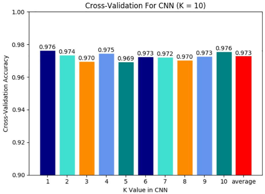
The accuracy using the 10-fold cross-validation.

Performance comparison

For comparison, the method proposed by S Hemminki et al.¹² was introduced in this section, and transportation pattern recognition accuracy is basically consistent with the accuracy stated in S Hemminki et al.¹² Comparative experimental results are shown in Figures 13 and 14. It is shown that the accuracy using the proposed algorithm is 14.71% higher than that of S Hemminki et al.¹²

Figure 13.

The confusion matrix using the method proposed by S Hemminki (average accuracy = 79.47%).

Figure 14.

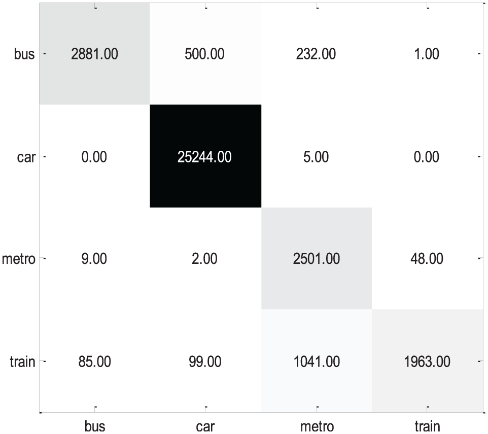
The confusion matrix using the proposed method (average accuracy = 94.18%).

Robustness

The robustness of transportation pattern recognition is greatly improved by the methods proposed in this article. The method presented in this article can be directly applied in various kinds of mobile phones.

Complexity analysis

The calculation complexity of our proposed algorithm is shown in equation (10)

o (\sum_{l = 1}^{d} n_{l - 1} • s_{l}^{2} • n_{l} • m_{l}^{2})

(10)

where d is the total number of plies in the network, $n_{l}$ is the number of convolutional filter in this layer; $n_{l - 1}$ is the upper layer convolution filter number; $s_{l}$ is the size of filter; and $m_{l}$ is the size of the output feature map

The above complexity is only theoretical, and the actual computation time is related to the mode of deployment and the hardware.

Pattern recognition performance

In this article, the accuracy rate is used to evaluate the performance of traffic pattern recognition algorithm. The accuracy rate of traditional algorithms, such as Adaboost, decision tree, random forest, and SVM, is compared and the comparison of different neural network structures is also conducted. In order to improve robustness use the proposed algorithm applicable to various mobile phones. In addition, deep learning algorithms are combined with the proposed sub-sensor structure, which can improve the efficiency of the proposed pattern recognition algorithm.

Conclusion

In this article, by introducing various features including semantic and sensory features, the proposed algorithm of TMD using CNN achieved accurate identification of various transportation mode. The greatest advantage of the proposed approach is the extraction of various semantic features, such as the frequency of turning and pause. These features are closely related to the specific transportation pattern as a whole and help differentiate various transportation patterns. From evaluation, using extracted high-level features can achieve higher pattern recognition accuracy than using the original data.

Compared with the random forest, SVM and Adaboost, CNN demonstrated the strongest learning ability and achieved the most accurate to identify transportation modes. The proposed algorithm is evaluated divided sensors and mixed sensors, individually and found that transportation estimation accuracy using divided sensors is higher than using mixed sensors.

Extensive experimental results report an average accuracy of 94.18% using the proposed algorithm based on the Keras framework. In addition, the system uses frame features and introduces only a few seconds of delay, and hence can be potentially useful for real-time applications, such as personal digital assistants. Given the ubiquity of these sensors on nowadays smart devices, this system has a great potential to be a low-cost and on-the-go solution for sensing people’s transit and further understanding human activities. In the future, the proposed algorithm will be implemented and evaluated on the commodity smartphones.

Footnotes

Handling Editor: Davide Brunelli

Declaration of conflicting interests

The author(s) declared no potential conflicts of interest with respect to the research, authorship, and/or publication of this article.

Funding

The author(s) disclosed receipt of the following financial support for the research, authorship, and/or publication of this article: This work was supported in part by the National Key Research and Development Program (2018YFB0505200), the National Natural Science Foundation of China (61872046), and the Open Project of the Beijing Key Laboratory of Mobile Computing and Pervasive Device.

References

Biancat

Brighenti

Review of transportation mode detection techniques. ICST Trans Ambient Syst 2014; 1(4): e7.

Parkka

Ermes

Korpipaa

et al . Activity classification using realistic data from wearable sensors. Proc IEEE Trans Inform Tech Biomed (A publication of the IEEE engineering in medicine & biology society) 2006; 10(1): 119–128.

Stenneth

Wolfson

et al . A method to determine a person’s mode of transportation (UIC-2012-115), https://flintbox.com/public/project/29113/

Gong

Zhao

Chen

A convolutional neural networks based transportation mode identification algorithm. In: Proceedings of the international conference on indoor positioning and indoor navigation (IPIN), Sapporo, Japan, 18–21 September 2017. New York: IEEE.

Reddy

Min

Burke

et al . Using mobile phones to determine transportation modes. ACM Trans Sens Netw 2010; 6(2): 13.

Widhalm

Nitsche

Brändie

Transport mode detection with realistic smartphone sensor data. In: Proceedings of the International Conference on Pattern Recognition (ICPR), Tsukuba, Japan, 11–15 November 2012, pp.573–576. New York: IEEE.

Shin

Aliaga

Tunçer

et al . Urban sensing: using smartphones for transportation mode classification. Comput Environ Urban 2014; 53: 76–86.

Huss

Beekhuizen

Kromhout

et al . Using GPS-derived speed patterns for recognition of transport modes in adults. Int J Health Geogr 2014; 13(1): 40.

Zheng

Chen

et al . Understanding transportation modes based on GPS data for web applications. ACM Trans Web 2010; 4(1): 1.

10.

Endo

Toda

Nishida

et al . Classifying spatial trajectories using representation learning. Int J Data Sci Anal 2016; 2(3–4): 107–117.

11.

Wang

Liu

Duan

et al . Detecting transportation modes using deep neural network. IEICE Trans Inf Syst 2017; E100: 1132–1135.

12.

Hemminki

Nurmi

Tarkoma

. Accelerometer-based transportation mode detection on smartphones. In: Proceedings of the ACM conference on embedded networked sensor systems, Rome, 11–15 November 2013, p.13. New York: ACM Press.

13.

Prentow

Blunck

Kjærgaard

et al . Towards indoor transportation mode detection using mobile sensing. In: Mobile computing, applications, and services: 7th international conference, Berlin, 12–13 November 2015. Berlin: Springer.

14.

Caceres

Tong

et al . Online travel mode identification using smartphones with battery saving considerations. IEEE Trans Intell Transp Syst 2016; 17: 2921–2934.

15.

Stenneth

Wolfson

et al . Transportation mode detection using mobile phones and GIS information. In: Proceedings of the ACM SIGSPATIAL international conference on advances in geographic information systems (GIS ‘11), Chicago, IL, 1–4 November 2011, pp.54–63. New York: ACM Press.

16.

Hemminki

. Transportation behavior sensing using smartphones. In: Proceedings of the ACM international joint conference on pervasive and ubiquitous computing (UbiComp), Zurich, 8–12 September 2013. New York: ACM Press.

17.

Qin

Jiang

Yuan

et al . Transportation mode recognition algorithm based on Bayesian voting. In: Proceedings of the 5th international conference on enterprise systems (ES), Beijing, China, 22–24 September 2017. New York: IEEE.

18.

Shafique

Hato

Use of acceleration data for transportation mode prediction. Transportation 2015; 42(1): 163–188.

19.

Feng

Timmermans

HJP

. Comparison of advanced imputation algorithms for detection of transportation mode and activity episode using GPS data. Transport Plan Techn 2016; 39(2): 180–194.

20.

Reddy

Burke

Estrin

et al . Determining transportation mode on mobile phones. In: Proceedings of the IEEE international symposium on wearable computers, Pittsburgh, PA, 28 September–1 October 2008, pp.25–28. New York: IEEE.

21.

Zheng

Liu

Wang

et al . Learning transportation mode from raw GPS data for geographic applications on the web. In: Proceedings of the international conference on World Wide Web (WWW), Beijing, China, 21–25 April 2008, pp.247–256. New York: ACM Press.

22.

Bengio

Lamblin

Popovici

et al . Greedy layer-wise training of deep networks. Adv Neural Inf Process Syst 2007; 19: 153.

23.

Mizell

Using gravity to estimate accelerometer orientation. In: Proceedings of the IEEE international symposium on wearable computers, White Plains, NY, 21–23 October 2003, pp.252–253. New York: IEEE.

24.

https://keras.io

25.

Frédéric

Pascal

Razvan

et al . Theano: new features and speed improvements. In: Deep learning and unsupervised feature learning NIPS 2012 workshop, Harrahs and Harveys, Lake Tahoe, 3–8 December 2012. New York: IEEE.

A traffic pattern detection algorithm based on multimodal sensing

Abstract

Keywords

Introduction

Related work

Transportation pattern detection

System architecture

Data preprocessing and feature extraction

Data pretreatment

Gravity estimation

Horizontal acceleration

Feature extraction

Acceleration features

Geomagnetic features

Pressure features

Static detection

Turning detection

The CNN architecture algorithm

Accelerometer feature

Gyroscope, geomagnetic, and barometric

Training phase

Test phase

Structure of the original data

Training phase

Test phase

Evaluation and analysis

Data sets

Performance evaluation

Algorithm comparison

Performance evaluation of different network architectures, parameters, and sensors

Influence of hyperparameter

10-Fold cross-validation

Performance comparison

Robustness

Complexity analysis

Pattern recognition performance

Conclusion

Footnotes

Declaration of conflicting interests

Funding

References