
Abstract
In view of the requirement on time synchronization for a kind of typical wireless sensor networks with long-chain-type topologies, taking into account the three-dimensional network model currently used by the localization algorithms, one feasible time synchronization algorithm is proposed in this article. Under the three-dimensional topology, nodes in the wireless sensor networks are divided into three kinds: the sensing nodes, the relay nodes, and the measured nodes. By analyzing the distribution characteristics of these three kinds of nodes, with the introduction of the pairwise broadcast synchronization and the series multi-hop synchronization protocol, the estimation of the clock offset and the clock skew of all the nodes in the wireless sensor networks are performed by virtue of the joint maximum likelihood and the least-squares method, thus the time synchronization of the wireless sensor networks with long-chain-type topology is solved. Moreover, the sink node evaluates the network periodically and adjusts the synchronizing cycle based on the difference between the network synchronization error and the given synchronization accuracy. The feasibility and effectiveness of this scheme are analyzed by simulations from the synchronization accuracy, the number of synchronization message, and the synchronizing cycle points of view.
Keywords
Introduction
Nowadays, wireless sensor networks (WSNs) are developed to provide fast, cheap, reliable, and scalable hardware solutions for a large number of industrial applications, ranging from surveillance and tracking to exploration, monitoring, and other sensing tasks. 1 Sensors can detect, measure, and collect information from various environments. 2 The information collected includes a variety of types, such as light, distance, vision, location, acceleration, sound, compass, rotation, magnetic, gravity, atmospheric pressure, temperature, and humidity. In many applications of WSNs, such as duty cycling, data fusion, localization, location-based monitoring, and routing, it is essential that the nodes in a network should act in a coordinated way, which implies all nodes must refer to a common notion of time, 3 that is to say, all the nodes in the network should be synchronized within the range of given synchronization errors. Moreover, the synchronization precision requirement is determined by the WSN’s application type, 4 and for the structures’ health monitoring scenario, the synchronization precision is to be around 0.25 ms, while for the location protocols, the precision needs to vary from 0.5 to 0.7 ms.
There is a special application scenario for WSNs: the underground supervision with long-chain-type topologies, 5 such as the underground utility tunnel supervision 6 and the underground coal mine supervision. 7 For this kind of WSNs, the wireless communication environments are supposed to be closed or semi-closed, and the communication channels are supposed to be the fading ones.8–10 Taking the underground coal mine supervision system as an example, the communication environment in coal mine is becoming more and more complex since the underground pressure, the high-level water pressure, and the coal mine gases are the main threats for the coal mine safety mining.
Since the underground WSNs have many special features, such as the long-chain-type topology, the complex wireless communication environment, and varying time, those traditional time synchronization methods, such as the reference broadcast synchronization (RBS),11,12 the flooding time synchronization protocol (FTSP),13,14 the timing-sync protocol for sensor networks (TPSN),15,16 and the average time-sync (ATS),17–19 are difficult to meet with the time synchronization requirements and cannot be applied directly to underground WSNs with long-chain-type topologies. The particularities of underground coal mine environment 20 put forward the active and passive time synchronization algorithm; 21 arrange all the perception layer nodes, including the sensing nodes and the measured nodes, along the hierarchical network structure; all the nodes acquire their time synchronization packet based on the overhearing mode. By analyzing the characteristics of WSN applications in underground coal mine and the particularities of the working face environment, based on the traditional FTSP time synchronization protocol and with the use of a threshold decision mechanism, 22 we proposed one fault-tolerant time synchronization algorithm.
Considering the characteristics of the coal mine tunnels, motivated by the network topology structure for the three-dimensional (3D) localization model proposed by Meng et al., 23 in this article, we propose one 3D-localization-based time synchronization method, and it has the following advantages:
Based on the currently used 3D model in underground coal mine, the network topology for time synchronization is somewhat easy to maintain, moreover with the use of the global long-term time synchronization for the network is realized in this article;
The sender and receiver synchronization (SRS) two-way exchange and the receiver only synchronization (ROS) one-way receive packet transmission mechanism are utilized together to synchronize nodes in the network, where the sensing nodes and the measured nodes in the network are synchronized with the one-way overhearing, thus the total synchronization packet for the WSN is largely decreased, which is more suitable for the scenario in underground WSNs;
With the use of network evaluation, we can make a good compromise between the synchronization precision and the energy consumption, thus the energy efficiency of the proposed time synchronization protocol gets somewhat improved.
The article is organized as follows. Section “Time synchronization for long-chain-type WSNs” introduces the time synchronization scheme based on the 3D localization model in coal mine tunnels. Sections “Time synchronization for relay nodes” and “Time synchronization for the sensing nodes and measured nodes” introduce the time synchronization for the relay nodes and the sensing (measured) nodes, respectively. The simulation results and the conclusion remarks are given in sections “Simulations” and “Conclusion,” respectively. The article is based on its previous version; 24 here, the results appear in improved forms along with more discussions.
Time synchronization for long-chain-type WSNs
In this section, based on the typically used 3D localization model, we mainly explain how to carry out our research on the time synchronization for WSNs in tunnels with long-narrow chain-type physical topology.
Network model
From the literature, 6 for WSNs in long-narrow chain-type tunnels, the wireless communication paths are narrow and staggered, meanwhile the tunnel’s top is a circular arc, thus those various types of nodes are often arranged in the hierarchical model. The 3D nodes’ arrangement is shown in Figure 1.

Three-dimensional model of long tunnels nodes’ arrangement.
In Figure 1, nodes arranged in the top of the circular arc are usually used as the relay nodes, which mainly obtain information from the sensing nodes within their communication range, with the use of proper data fusion and then relay those fused information to the sink node in a multi-hope way. When it comes to the sink node, also called the gateway node, it is usually arranged in the entrance of the tunnels and can communicate with the backbone network through the means of wired communication. Moreover, the sensing nodes are arranged in the four oblique vertical angles of the rectangular and are usually used as the detection nodes. As for the measured nodes, they are usually carried by the moving persons, the moving machine, or the moving equipment, thus they are different from those static nodes mentioned above; they are dynamic nodes and their movements may be random. 25
Clock model and time synchronization definition
In the WSNs, assuming that the clock of each node i has one oscillator that can be capable of incrementing a tick counter by one tick. The real period

where

where

where
Note that a hardware clock value

where
Substituting equations (1) in (3), one can get

where
Definition
For a WSN with N nodes and one sink node g, if, for any initial conditions

then all the N nodes are synchronized to the sink node g, and the network WSN is said to have achieved its time synchronization.
Chain-type topology construction
In this article, we adopt the typically used 3D long-chain structure to construct the communication topology for time synchronization and utilize both the SRS two-way exchange and the ROS one-way receive packet transmission mechanism; the constructed communication topology for the long-chain-type tunnel is shown in Figure 2. The construction for the long-chain topology for time synchronization consists of the following steps:
The sink node, arranged in the entrance of the long-chain-type tunnel, is used as the root node, which is allocated to level 0 and broadcasts a level-discovery packet to its neighbors that contains its identification code and level;
When the subsequent relay node receives the node level-discovery packets, it allocates a level for itself which equals 1 plus the smallest one of the level numbers it extracted from all the tunnels’ level-discovery packets;
The subsequent relay node broadcasts a level-discovery packet containing this new level, and this process will get performed until the end relay node has obtained its level number and has determined which sink node it belongs to.

Topology for WSNs in long-chain-type tunnels.
The simplified topology with two communication chains is shown in Figure 3, where

Simplified chain-type network with two sink nodes.
Time synchronization for WSNs
In this article, we utilize the pairwise broadcast synchronization (PBS) method, that is, the two-way exchange and one-way overhear model, to realize the time information exchange among nodes in WSNs, where the information is two-way exchanged between the relay nodes, besides the sink node, and the sensing nodes and the measured nodes overhear those information in a one-way overhearing one. In one synchronization cycle, we exchange N packets between the relay nodes, and the ith synchronization packet exchange is shown in Figure 4, where a and b denote the relay nodes (besides the sink node), while s denotes the sensing node or the measured nodes.

RSR two-way exchange and the ROS one-way receive synchronization packet transmit model.
In Figure 4, during the ith synchronization packet exchange phase, timestamps
Assuming that the transmission delay between nodes are Gaussian distributed ones, based on the data obtained from information exchange, all nodes in WSNs can adopt the joint maximum likelihood estimation (JMLE) algorithm or the least-squares method to estimate the clock skew and offset among nodes in the network, 29 therefore the time synchronization of the network is achieved.
Time synchronization for relay nodes
In this section, based on the information exchange model shown in Figure 4, we will introduce the synchronization method for the relay nodes, including the following two stages: the single-hop synchronization stage and the multi-hop synchronization stage.
Single-hop synchronization
Assuming that the transmission delay between nodes obeys Gaussian distribution, based on the data obtained from information exchange, in this section, we adopt the JMLE algorithm to estimate the clock skew and offset among nodes in the network. 29
With
Assuming that

When the fixed transmission delay

From equation (8), the JMLE of the clock offset and skew can be calculated as

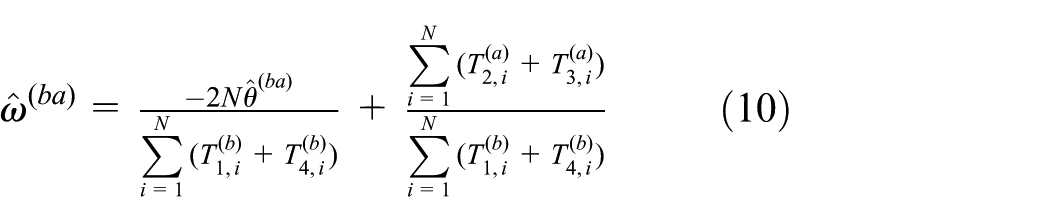
where
Multi-hop synchronization
In this section, we continue to explain how to realize the multi-hop synchronization for the relay nodes. Here, we adopt the series multi-hop synchronization algorithm (SMA) to achieve the multi-hop time synchronization of relay nodes, and the synchronization strategy is shown in Figure 5.

Continuous multi-hop synchronization model.
In Figure 5, node 3 delivers the synchronization packet SYN, containing a time stamp
From what we have stated above, the clock expression of any relay node to the sink node on a chain link can be expressed as
Time synchronization for the sensing nodes and measured nodes
It has been mentioned before that, the measured nodes are usually objects which are need to be positioned, and select to synchronize or not to the sink node according to actual demands. Therefore, the synchronization method for measured nodes are similar to that of sensing nodes. For the case of brevity, in this section, we will introduce the time synchronization method for both the sensing nodes and measured nodes in the network simultaneously.
Similar as the synchronization method for those relay nodes, here, we also divide the time synchronization into two stages: the single-hop stage and the multi-hope stage.
Single-hop synchronization
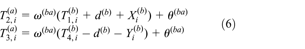
In Figure 4, when considering the influence of clock offset and skew simultaneously, in the ith uplink information, the receiving time

and

where
Subtracting equation (12) from equation (11), we can derive

where
Let us continue to introduce how to use the linear regression method to estimate the clock offset of sensing (measured) node s with respect to the relay node a. In equation (13), denote

Utilizing the least-squares method yields

and
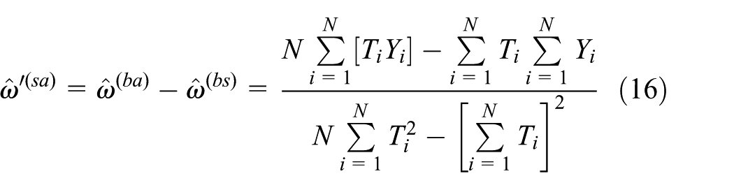
With the above conclusion, the estimation results of the difference between the relative clock offset and skew can be obtained.
Since the relative clock relationship between nodes b and a, and nodes b and node s can be expressed as

and

the relative clock offset and skew between nodes s and a are in the following form
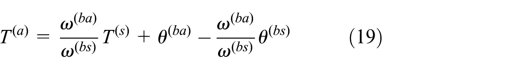
From equation (19), we can write the clock offset and skew between nodes s and a in the following form

and

It should be mentioned that
Multi-hop synchronization
It can be seen from Figure 2 that, when the level
and

where
and

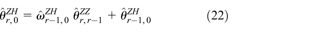
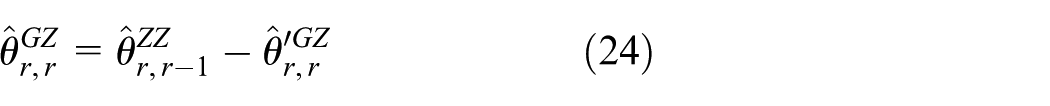
Referring to equation (19), we can also deduce the general expression about the clock offset and clock skew between level r sensing (measured) node and level


Therefore, the clock offset and clock skew between the level r sensing (measured) node and the sink node are shown as

and

Thus, the synchronization between the sensing (measured) nodes and the sink node has been finished.
Network evaluation
When designing the time synchronization algorithm for WSNs, there are many important factors to be considered, such as the synchronization precision and the energy consumption, which may compromise with each other. For nodes in WSNs, in many contexts, it is hard to recharge the batteries or scavenge energy from the environment, so when designing the time synchronization parameters, such as the synchronization period τ, the number of synchronization packets N transmitted during one period and so on, one of the most crucial factors to be considered is the energy consumption; 30 the smaller the τ, the lower the synchronization error, but more the energy consumption. The accuracy of the time synchronization to large extent is determined by the synchronization period. For example, according to Elson et al., 11 assuming that the upper limit of the clock synchronization accuracy is 10 ms, and in the most crucial case, the synchronization error is 50 µs, together with the clock skew is 4.75 ppm, then the maximum synchronization period can be calculated as

In this article, we propose one easy way to realize the method which is to regulate the synchronization period τ according to the synchronization error e(t) performed by the sink node during the network evaluation phase. For level i, define the synchronization error with respect to the sink node g

where

and
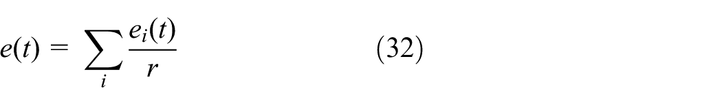
where r is the maximum level of the considered network and is determined during the topology construction phase.
The network evaluation is launched by the sink node g, and the evaluation is performed as follows:
When the sink node g wants to evaluate the network, all the nodes b in Figure 4 embed one special symbol to the SYN packet;
All the nodes s in Figure 4 acquire this symbol from the SYN packet, and after they have estimated the clock skew and clock offset, they send these two estimations to the relay node at the same level;
The relay node at the level obtains the synchronization error of sensing (measured) node to the sink node (which means the reference time) according to equation (31), then calculates the average synchronization error of this level based on equation (30), and delivers this average error to the sink node with the aid of all the top level relay nodes;
The sink node g receives all the
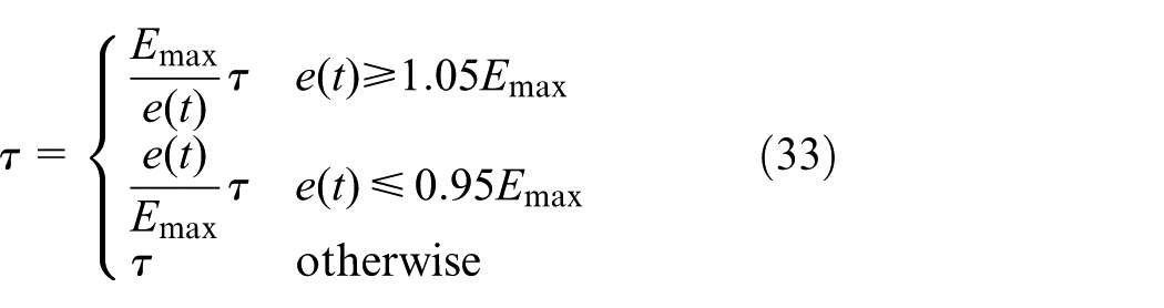
so as not to only meet with the clock synchronization accuracy requirements
Simulations
In this section, we will illustrate the proposed time synchronization method for WSNs via some numerical simulations. All the figures and table are drawn from the results of the average over 1000 runs with the randomized initial conditions.
We set the simulation parameters, such as the mean and the variance of the Gaussian distribution RVs, based on Table 1 in the literature, 15 and set them as follows: the random delay is set to Gaussian distribution with the mean 2.5 µs and variance 1 µs, and the fixed delay is d = 1 µs.
Statistics of synchronization error (only magnitude).

TPSN: timing-sync protocol for sensor networks; RBS: reference broadcast synchronization.
According to the features of long-chain-type tunnel, during the simulation, we denote the height and width of the tunnel both to be 6 m, then the topology of a tunnel with 100-m length is shown in Figure 6, with 1 sink node, 5 relay nodes, and 27 sensing (measured) nodes, the communication ranges between the sink node and the relay node is 21 m, and the range between the sensing node and the measured node is 12 m.

Network simulation topology.
Effectiveness of the proposed algorithm
In this section, we will show the effectiveness of the proposed time synchronization method for the relay and sensing nodes. It should be mentioned that TPSN method has not estimated the clock skews between nodes and it is a short-time synchronization method. The comparisons on the mean square errors (MSEs) of the clock offset and the skew estimation with respect to the synchronization packet number N among the relay nodes, the sensing nodes in this article, and the errors of the TPSN method proposed in Ganeriwal et al.
15
are shown in Figure 7(a) and (b), respectively, where the MSEs of the clock offset and the skew estimation are defined as

Mean square error curves of the clock estimations: (a) offset estimation (MSE) and (b) skew estimation (MSE).
It can be seen from Figure 7 that:
With the increase in synchronization packet number N, the MSEs of the clock offset and skew estimations of relay and sensing nodes of this article all showed decreasing trends, which means that the more the value of N, the closer their estimation values to the actual clock offset and skew;
The convergence speed of the estimation MSE curves for the relay nodes and sensing nodes is different, since they use different methods to estimate the clock skews and offsets, and the speed of the pairwise synchronization SRS mechanism adopted by relay nodes is faster than that of the overhearing ROS mechanism adopted by the sensing nodes.
Comparisons on
Denote the synchronization packet number in one period as N, and the total packet number for the WSN as
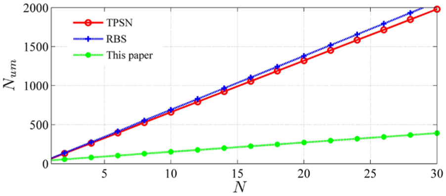
Comparisons on
It can be seen from Figure 8 that, for the long-chain-type topology in underground WSNs, the protocol proposed by this article deserves the least synchronization overhead and can save most of the energy, thus it is more suitable for the underground WSNs.
Network evaluation
We first set the synchronization accuracy as 1 ms and run the protocol for 100 cycles, then change the accuracy to 0.1 ms and run the protocol for another 100 cycles, where the simulation time is 22513.5 s and the network is evaluated by the sink node every 10 cycles. The curves for synchronization error and the synchronizing cycle are shown in Figure 9.

Curves for synchronizing cycle τ adaption and the synchronization error e.
It can be seen from Figure 9 that (1) the synchronization error can change with the change in
Conclusion
Aimed at the requirement of time synchronization for one long-chain-type WSNs in underground coal mines, taking advantage of the currently used 3D localization model in the tunnels, one feasible time synchronization scheme is proposed in this article and its effectiveness is verified by simulations. The time synchronization is solved with the joint use of SRS and ROS packet transmission mechanism, thus the number of synchronization packet gets greatly decreased, which means that the energy efficiency gets improved. The estimation of clock skew and clock offset relative to the sink node is carried out by virtue of the joint maximum likelihood and the least-squares method, thus the global time synchronization of the WSN is realized. During the network evaluation phase, the synchronizing cycle in the whole network is adjusted according to the difference between the accuracy requirement and the realtime synchronization error, so that the energy consumption gets further reduced. Therefore, the proposed protocol can make a good compromise between the synchronization precision and the energy consumption.
As a preliminary study, this article just describes the general process of the adaptive adjustment of the entire network and has not analyzed it systematically, which is the main task for our future works. We will verify the effectiveness of the proposed method in the hardware sensor nodes.
Footnotes
Handling Editor: Pengpeng Chen
Declaration of conflicting interests
The author(s) declared no potential conflicts of interest with respect to the research, authorship, and/or publication of this article.
Funding
The author(s) disclosed receipt of the following financial support for the research, authorship, and/or publication of this article: This work was supported by the National Natural Science Foundation (NNSF) of China under grant nos 51874205, 51274011, and 61472003; Jiangsu Natural Science Research Major Projects in Colleges and Universities under grant no. 17KJA520005; and Suzhou University of Science and Technology Talents Research Funding Project under grant nos 331711602 and 491811104.