Sage Journals: Discover world-class research

Abstract

We have developed a maximum likelihood formulation for a joint detection, tracking and association problem. An efficient non-combinatorial algorithm for this problem is developed in case of strong clutter for radar data. By using an iterative procedure of the dynamic logic process “from vague-to-crisp” explained in the paper, the new tracker overcomes the combinatorial complexity of tracking in highly-cluttered scenarios and results in an orders-of-magnitude improvement in signal-to-clutter ratio.

Keywords

Maximum Likelihood Joint Association Tracking and Detection Combinatorial Complexity Tracking Association Clutter Weak Targets Strong Clutter

1. Introduction

Performance of state-of-the-art algorithms for tracking and association in strong clutter [1], as a function of Signal-to-Clutter Ratio (SCR), is significantly below the information-theoretic limit as indicated by the Cramer-Rao Bound (CRB) for tracking in clutter [2]. The reason for this underperformance is the combinatorial complexity of algorithms. When clutter is strong, so that the signals are below clutter, two tasks have to be performed concurrently. First, a tracking algorithm has to decide which signals come from the tracked object and which come from clutter. Secondly, track parameters (position, velocity, etc.) have to be estimated. The only information to solve the first problem comes from the second one: track signals form a reasonable track. Therefore both parts of the problem have to be solved concurrently. This requires consideration of multiple associations between data and tracks concurrently with detections. In other words detection, association and tracking should be performed jointly. The number of associations grows combinatorially with the number of data points (every point could be associated with many points in the next scan and each point could be associated with many points again and again). Therefore performance is limited by the complexity of computations rather than by the information in the data. Here we describe a non-combinatorial solution of the maximum likelihood (ML) joint tracking and association problem resulting in a significantly improved performance. Part of this paper has been presented at the lecture [3,4]. The fundamentally novel contributions of this paper includes the ML formulation of the joint detection, association and tracking problem, its non-combinatorial solution and an intuitive discussion of what enabled this improvement; we also compare this algorithm to the performance of other published tracker results.

The neural network tracker developed in [5] addressed the problem of tracking a manoeuvring target, a different problem to tracking in clutter considered here. A combination of particle filters and the likelihood of target appearance were developed for tracking in [6,7]. However, in strong clutter particle filters lead to NP (nondeterministic polynomial (time)) complexity [8,9] and cannot solve the problem of tracking in clutter. Ensemble-based learning was developed for tracking and fusion in [10], however, tracking in strong clutter was not addressed. A combination of Gaussian mixtures and Kalman filter tracking was used in [11], yet “motion detection and tracking in a cluttered environment experience many problems.” In [12] cooperative sensor networks were considered, however, tracking in clutter was not specifically addressed. Algorithms specifically addressing tracking in clutter include Multiple Hypotheses Testing (MHT) [13] a standard algorithm used in current radar detection and tracking subsystems. It operates in a two-step process. First, Doppler peaks are detected that exceed a predetermined threshold. Second, these potential target peaks are used to initiate tracks. This two-step procedure is a state-of-the-art approach which is currently used by most tracking systems. The limitation of this procedure is determined by the detection threshold. If the threshold is reduced, the number of detected peaks grows quickly. Increased computer power does not help because the processing requirements are combinatorial in terms of the number of peaks, so that a tenfold increase in the number of peaks results in a billion fold increase in the required computer power. Therefore developing algorithms capable of non-combinatorial joint detection, association and tracking is a desirable goal. Before describing such an algorithm below, we briefly review previous development.

The idea of probabilistic association originated from Bar-Shalom's JPDAF (joint probabilistic joint data association filter), [14], which is more efficient than MHT because one only needs to evaluate the association probabilities separately at each time step. However, since all data association mappings are not considered, this method is not optimal [15,16]. Also, JPDAF cannot be used for track initialization since detection is performed separately from tracking, whereas optimum performance is only obtained when detection and tracking are performed concurrently [2,17,18,19].

In the approach described here, data association is performed concurrently with detection and tracking without a combinatorial explosion in computational requirements. Also, the approach is appropriate for handling low SCR data and data with multiple, closely-spaced and overlapping targets. Whereas MHT is based upon selecting the best data-to-target mapping to calculate the track parameters, the method described here associates data with target and clutter components probabilistically and does not require selection of the best data-to-target mapping. Here, the track parameters for a particular target are computed using a weighted combination of all data samples, where the weights correspond to the association probabilities. The advantage of this framework can be understood by comparing it to “hill climbing” optimization, which does not account for associations between data, track and clutter; the current procedure is significantly more efficient than “hill climbing” optimization, it is performed in the space of all model parameters and all possible mapping-associations between data samples, clutter and targets. Some aspects of this procedure are similar to the expectation-maximization (EM) algorithm [20,21,22,23], with a fundamental difference discussed below (see also [22]). The algorithm discussed here is optimal [2,17,18,24,25]. A minor improvement over MHT is that, despite a complete search, MHT is optimal only under certain assumptions as discussed in [25]. The major improvement is that whereas the computational complexity of MHT scales exponentially with the number of targets, data samples and sensors, the method described here scales only linearly with each of these parameters. Therefore MHT cannot be used in strong clutter and requires the target signals to be much stronger than the clutter, whereas the algorithm described here can detect and track even when the target signals are below the clutter; as discussed below the improvement could be up to 2 orders of magnitude or more.

The general framework for the approach described in this paper was developed by Perlovsky in his work on multi-target tracking in clutter, automatic target recognition (ATR) and sensor fusion [2,19,25,26,27], (and other references contained in [25]).

In these references it has been recognized that if classification features are available, an optimum algorithm will perform target classification concurrently with detection and tracking, by mathematically placing the tracking coordinates (range, Doppler, bearing) on an equal footing with the classification features. Thus, a composite model of the data can be expressed as a mixture of track and clutter model components in the combined space of tracking and classification features. The algorithm described here is based upon this general approach [25,26,27] which we refer to as dynamic logic (DL) for the reason discussed below. Although the general formulation enables the use of classification features, the examples considered in this paper do not make use of any classification features.

Other algorithms developed after DL have some superficial similarity to DL and should be mentioned for the completeness of this short review. The probabilistic multihypothesis tracker (PMHT) [28,29] was developed by Streit and Luginbuhl and it shares strong similarities with Avitzour's approach [30]. A similarity between DL and these other trackers is that they use EM to perform data association probabilistically, while simultaneously estimating track parameters and yet, the manner in which EM is used is fundamentally different, DL does not treat associations (or any other variables) as “missing variables”, the hallmark of EM. The most important difference is that DL has linear complexity, whereas all other algorithms have exponential or combinatorial complexity; this is responsible for the DL's significant improvement in performance (orders of magnitude in terms of signal-to-clutter ratio).

The DL tracker is a “Track-Before-Detect” algorithm, it simultaneously performs data detection, association and track estimation; it uses either unthresholded sensor data or thresholded data with a very low threshold. This increases the measurement data set by orders of magnitude and increases the number of associations astronomically (and worse), yet the DL tracker can handle the large amount of data, because of its linear (non-combinatorial) complexity. It operates on data measured over several frames in a batch algorithm to obtain a track estimate. When applied to a benchmark multi-target tracking problem, it was found that the computational cost of PMHT has roughly the same (exponential) order of magnitude as the cost of MHT, PDA (Probabilistic Data Association) and JPDAF [16]. As mentioned above, the computational cost of the DL tracker scales only linearly with increasing numbers of measurements and sensors, whereas the cost of MHT and other algorithms scales exponentially. This cost advantage of the DL tracker is even more evident for the multi-sensor case [24,25,31,32,33,34,35,36,37,38]. This linear complexity of DL vs. exponential complexity of other algorithms is the main topic of this paper.

The paper is organized as follows. In Section II the likelihood function is derived for joint tracking and association, Section III formulates the DL equations for non-combinatorial maximization of the likelihood. Section IV demonstrates performance examples. Section V discusses future research directions.

2. Likelihood for Joint Tracking and Association

Consider k radar scans, resulting in n = 1… N measurements X(n) = (x_n, y_n, a_n, D_n) where (x_n, y_n) are range and cross-range positions, an is amplitude and Dn is Doppler. Measurements n = 1… N include all the data used for estimation, what is often called a batch (for a better intuitive understanding of the following equations, let me emphasize that the relationship between scan number k, measurement number n and the time of measurement n, tn may be nontrivial). In a simple case, measurements taken during a single scan k might be considered co-temporal (same time tn corresponding to one scan). But in general this is not so. Nevertheless, the notation used below does not depend on this relationship; in fact, k does not need to be used at all. With our notation, extension to multi-sensor tracking is easily achieved [25,32,37].)

A likelihood of error measurement, e(n) is defined as follows: error measurements are considered independent, therefore, according to the standard probabilistic procedure for independent data [39,40] the joint probability density function (pdf), or likelihood is defined as

L ({e (n)}) = \prod_{n \in N} pdf (e (n)) .

(1)

Here Π stands for a product over n = 1… N. A pdf(e(n)) is defined according to multiple hypotheses (note a difference in terminology, in an MHT algorithm a hypothesis is every association between data and track; we call a hypothesis a track or clutter with unknown parameters). The measurement X(n) can originate from clutter, or from one of several moving objects, which are the alternative hypotheses. We number hypotheses h = 1…H; h=1 corresponds to clutter, h = 2…H correspond to H-1 tracks. According to the standard probabilistic procedure for alternative hypotheses [39,3407]:

pdf (e (n)) = \sum_{h \in H} r (h) pdf (e (n) ∣ h),

(2)

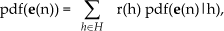
Here Σ stands for a sum over h = 1… H; r(h) is an a priori probability that measurement n originates according to hypothesis h and pdf(e(n)|h) is a conditional pdf for this hypothesis. Let us emphasize that there is no explicit mathematical expression for e(n), only pdf(e(n)) can be defined as in eq.(2). In this way e(n) is no different from any random variable defined under multiple hypotheses [39,40]. Substituting eq.(2) into eq.(1), we obtain:

L ({e (n)}) = \prod_{n \in N} \sum_{h \in H} r (h) pdf (e (n) ∣ h) .

(3)

This expression defines the likelihood in the context of multi-hypotheses tracking accounting for unknown tracks as well as for unknown associations of data and tracks (and clutter as well); this have been an unsolved problem in the past. Note, a priori probabilities r(h) are unknown and have to be estimated from the data the same as other unknown parameters. This product of sums contains H^N items corresponding to all combinations of data and tracks or clutter (every data point could have originated according to any hypotheses). This huge number is the reason for the combinatorial complexity of algorithms in the past. The above notation for conditional pdfs is a shorthand for pdf(e(n)| M_h(n)), where M_h(n) is a model predicting measurement X(n); if this measurement originates according to hypothesis h, then M_h(n) is an expected value of this measurement (when true parameter values are used):

M_{h} (n) = E {X (n) ∣ h},

(4)

and

e (n,h) = X (n) - M_{h} (n) .

(5)

We consider tracking short track segments, tracklets, along which velocities can be considered constant V_h = (V_hx, V_hy). Correspondingly, the complete model is:

M_{h} (S_{h},n) {= (X0}_{h} {+V}_{hx} t_{n} {, Y0}_{h} {+V}_{hy} t_{n} {, a}_{h} {, D}_{h}) .

(6)

Here parameters of the model, S_h = (X0_h, Y0_h, V_hx, V_hy, a_h, D_h); (X0_h, Y0_h) model an original position, (V_hx, V_hy) model velocity, (a_h, D_h) model amplitude and Doppler; t_n is the known time counted from the first scan. Also:

V_{hx} {= D}_{h} .

(7)

The unknown parameters include r(h), parameters of conditional pdf, such as standard deviations or covariances and the total number of track-models. Conditional pdfs for clutter we define as uniform:

pdf (X (n) |1) = 1 ∕ par_volume,

(8)

where par_volume is a volume of the parameter space, a product of (S_max – S_min) for all parameters. Conditional pdfs of tracks are defined as Gaussian; we would emphasize that it is different in principle from so called “Gaussian assumption” since we do not assume that the data are Gaussian. In view of hard boundaries S_max, S_min, this is an approximation; also parameters a_h are not likely to follow Gaussian distributions. In our practical cases this approximate treatment has been sufficient:

\begin{array}{l} pdf (e (n,h) ∣ h) = {(2π)}^{-2} {({det C}_{h})}^{-0 . 5} \\ exp{-0.5e {(n,h)}^{T} C_{h} ​^{-1} e (n,h)} . \end{array}

(9)

We use diagonal covariance matrixes C_h=diag(σ_xh²,σ_yh²,σ_ah²,σ_Dh²); and σ_xh²=σ_Dh². This covariance matrix combines the uncertainties of the states and measurements.

3. Dynamic logic

Now we describe a procedure (an algorithm) to maximize the likelihood (1) while at the same time solving the association-assignment problem without combinatorial complexity. We call this procedure dynamic logic (DL) for reasons described in [25,32,41]. The following algorithmic iterative equations (10) through (17) follow derivation in [25], where the local convergence is proven.

DL is an iterative procedure, which starts with unknown values of model parameters and correspondingly large uncertainty of associations; this later requirement is achieved by setting the standard deviation of parameters equal to one half of the (max – min) value for these parameters (which are usually approximately known in an operation scenario). Taking these initial values of parameters, conditional probabilities eq.(9) are computed. Then association variables, f(h|n), are computed; they are defined similarly to Bayesian posterior probabilities (for shortness, we use indexes n and h instead of the corresponding data X(n) and models M_h(n)):

f (h|n) = r (h) pdf (n|h) ∕ \sum_{h^{'} \in H} r (h^{'}) pdf (h^{'}) .

(10)

Although eq.(10) looks like Bayesian posterior probabilities, initially f(h|n) are not probabilities, since the parameter values are incorrect; they can be called association variables or estimated probabilities of measurements n originating from tracks (objects or hypotheses) h.

The next step is to estimate parameters using these estimated association probabilities. The equation for r(h):

r (h) = \sum_{n \in N} ​ f (h|n) /N .

(11)

This gives an estimated average ratio of data points assigned to track h (or clutter h=1) to the total number of data points N. This and other parameter estimation equations look simpler with the following notations. For any function G(h,n), introduce a weighted average over n, conditioned on h:

< G (h,n) >_{h} = \sum_{n \in N} f (h|n) G (h,n) ∕ N .

(12)

Then eq.(11) can be rewritten as:

r (h) {= < 1 >}_{h} .

(13)

Other parameter estimation equations at each iteration are computed as:

a_{h} {= < a}_{n} >_{h} .

(14)

(Eqs.(13) and (14) admit easy interpretations. The prior r(h) is a weighted average proportion of the number of data points associated with hypothesis h, according to the current values of association probabilities f(h|n). Similarly a_h is a weighted average amplitude of the data points associated with hypothesis h:

\begin{array}{l} {Y0}_{h} {< 1}_{​} >_{h} {+ V}_{yh} {< t}_{n} >_{h} {= < Y}_{n} >_{h}, \\ {Y0}_{h} {< t}_{n} >_{h} {+ V}_{yh} {< t}_{n} ​^{2} >_{h} {= < Y}_{n} t_{n} >_{h} . \end{array}

(15)

\begin{array}{c} {X0}_{h} {< 1}_{​} >_{h} V_{x_{h}} {< t}_{n} >_{h} {= < X}_{n} >_{h}, \\ {X0}_{h} {< t}_{n} >_{h} V_{x_{h}} ({< t}_{n} ​^{2} >_{h} + c < 1 >) = \\ {= < X}_{n} t_{n} >_{h} {+ c < D}_{n} >_{h} . \end{array}

(16)

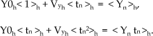
Here, c=σ_xh²/σ_Dh². For the unknown parameters Y0_h and V_yh eq.(15) is a two-dimensional linear system of equations; similarly eq.(16) is a two-dimensional linear system of equations for X0_h and V_xh. Standard deviations for each parameter s are estimated, as follows:

σ_{hs} ​^{2} {= < (X}_{s} (n) {-M}_{hs} (n))^{2} ​_{​} >_{h}

(17)

DL consists of iterative computations of eqs.(10) through (17). When the estimated parameters are far from the true values, the models do not match the data: standard deviations are large and the associations f(h|n) are “flat”, there are small numbers for many combinations of n and h (including incorrect ones) and any data point has a nonzero assignment to any track (or clutter). Nevertheless, even with these poor initial associations the parameter values improve with each iteration according to a theorem proven in [22]: likelihood (1) grows with every iteration and the DL procedure converges (local vs. global convergence is discussed below). As parameter values converge close to their true values, standard deviations converge to small values close to those of the sensor errors. Association variables converge close to true probabilities, close to 1 for n and h pairs corresponding to data n originating from object h and to 0 otherwise (this last statement is true to the extent that the information contained in the data is sufficient for track separability and data association). This DL process from vague to crisp associations is characteristic of DL [25,32,42].

Before proceeding with a detailed discussion, in the next three paragraphs we describe the above procedure in a simplified way for better intuitive understanding of the DL procedure.

An intuitive suggestion for eqs.(14) through (17) can be obtained by taking derivatives of the likelihood, eq.(3), with respect to the unknown model parameters and their standard deviations and setting each derivative to 0. Of course, this procedure does not prove anything; it is just an intuitive suggestion. The proof that iterations using these equations converge is discussed in [23]. These equations are much simplified in cases when there is just one track and no clutter. Then there is just one track hypothesis, all f(h|n) =1, hypothesis index h is not needed and weighted averages with brackets <G> become just regular averages. In this case, e.g., r = 1 and a = average amplitude of all data points. In eqs.(11) through (17) all unknown parameters are on the left hand side; equations for the parameters become linear, they are solved straightforwardly giving parameters of the track and no iterations are needed.

Next, consider a batch of data including all the data from 6 scans. Assume we know that there is just one track, h=2, resulting in no more than 6 data points and many clutter points randomly scattered over the X and Y coordinates. If the amplitudes and Doppler of track signals are below the average clutter amplitude and Doppler, the problem is very complex and previously could not have been solved. We initiate DL iterations with a uniform clutter model, h=1, over the entire span of the X and Y coordinates; with the amplitude and amplitude standard deviation (std), a(1) and std_a(1), computed as an average and std of all data and with an approximately known prior probability r(1) = (N-6) / N. The track prior is initiated to r(2) = 1-r(1) = 6 / N. We initiate the track position (X0, Y0) at the centre of the distribution of all data points and velocity, (Vx, Vy), is initiated at 0. Standard deviations of track parameters are initiated according to the uncertainty of this knowledge, for X0, std(2) = X_max - X_min; and similarly for Y0; std for velocity components is initiated to std(2) / (t_max-t_min); the signal amplitude and std are initiated equal to those given by the clutter. To summarize, all parameters and their stds are initiated according to the absence of any knowledge. With all parameters defined, all pdfs can be computed eqs.(8), (9).

On the first iteration we consider all data points as belonging to the track with probabilities corresponding to eq.(10). This is not much different from considering all data points approximately belonging to the track; minor deviations, even if random, are still necessary, as is clear from the following. Given these associations we can estimate new values of parameters positions, velocities, etc., according to eqs.(11) through (17). According to the proof in [25] the likelihood increases, which can be intuitively simplified as an improvement of model parameters and correspondingly a decrease of stds and track error ellipses in (X, Y). (3) On the second iteration the size of the error ellipse is smaller and fewer data points are significantly associated with the track (Note, this requires that f(2|n) are not exactly 1 on the first iterations, otherwise nothing will change). The estimation procedure (2.) is repeated, resulting in a larger likelihood, better parameter values, smaller stds and a smaller track error ellipse. After several iterations, parameters get very close to their true values, the track error ellipse becomes very narrow around the true track, association probabilities f(h|n) eq.(10) become 0 or 1 for the correct data-model associations (track or clutter) and iterations stop improving. The problem is solved, no combinatorial complexity is encountered. Let us emphasize that this paragraph gives an approximate, intuitively correct description of the DL process. The maximum likelihood increase on every iteration is a mathematically exact statement [25].

The computational complexity of the DL procedure described above is proportional to the number of data points and the number of tracks, const*N*H. The const here accounts for the number of iterations, it, and for the complexity of the procedures described by (10) through (17), const ∼ 10*it, where it is a number of iterations. Typical numbers of iterations, it, are discussed in the next section. The principal theoretical moment is that this number is linear in N and in H, rather than combinatorial, ∼H^N like in MHT.

The number of tracks is estimated as follows. The algorithm starts with 1 active track model, whose parameters are updated from iteration to iteration. In addition, the algorithm keeps one (or several) dormant track, whose parameters are not updated, except for r(h). On the 1^st iteration all standard deviations are large and the track and clutter models have low but nonzero associations to all data points. After a few iterations the active track standard deviations become smaller, there is a stronger association with some returns and a weaker association with others. According to eq.(11), sum the total associations of every data point n, Σhf(h|n) = 1; therefore some associations for dormant tracks grow. After r(h) for a dormant track exceeds a predetermined threshold, this track is activated and its parameters are updated. Similarly, if r(h) falls below the threshold, the track is eliminated. In this way as many tracks are activated as justified by the data. This procedure may lead to too many active tracks. When standard deviations approach sensor error values and association variables approach 0s and 1s, extra tracks tend to converge either on top of each other, or to one or two data points, these are pruned. Upon convergence (likelihood eq.(1) increase between iterations become less than a threshold), a detection measure is computed for each track; it is defined as a local log-likelihood ratio computed using returns within two standard deviations {n′} of each track:

LLR (h) = \sum_{n^{'} \in N^{'}} [ln pdf (n^{'} |h) - ln pdf (n^{'} |1)] .

(18)

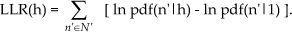
Tracks with LLR(h) exceeding a predetermined threshold are declared detections.

Convergence of this iterative procedure to a local maximum of likelihood (1), as mentioned, was proven in [25]. Such local convergence usually occurs within relatively few iterations; a typical example in the next section took 20 iterations. Since likelihood is a highly nonlinear function, regular convergence to the global maximum cannot be expected. The local rather than global convergence sometimes presents an irresolvable difficulty in many applications. In the presented method, this problem is addressed in several ways. First, the large initial standard deviation of the likelihood smoothes local maxima. Second, tracks are pruned and activated as needed. Therefore if a particular real track is not “captured” after few iterations, it will be captured at a later iteration after a track-model activation. Third, if a spurious track is declared detected, or a real track is missed, these errors will be self-corrected at a later stage of a system operation, when detected track segments or tracklets are connected into longer tracks (system operation procedures are beyond the current communication; we would add that the second and third considerations above are relevant for system operation performance, independent of reaching global maxima on each run).

4. Tracking example and Operating Curves

An application example of the above described DL tracker is illustrated in Fig. 1, where detection and tracking are performed for targets below the clutter level. Fig. 1(a) shows true track positions in a 0.5km * 0.5km data set, while Fig. 1(b) shows the actual data available for detection and tracking. In these data, the target returns are buried in the clutter, with signal-to-clutter ratio of about −2dB for amplitude and −3dB for Doppler. Clutter points are random throughout the entire data set, they do not move on any tracks and are not repeated from scan to scan. Let us emphasize, target returns are lower than clutter returns and cannot be visible, this does not depend on renormalizing image brightness; similarly, the track points are not visible when looking at the sequence of 6 scans. The problem cannot be simplified by dividing the tracking area into smaller pieces, since positions of targets and track lengths are unknown. Here, the data are displayed such that all six revisit scans are shown superimposed in the 0.5km * 0.5km area, 500 pre-detected signals per scan and the brightness of each data sample is proportional to its measured Doppler value. Figs. 1(c)-1(h) illustrate the dynamics of the algorithm as it adapts during increasing iterations; the brightness is proportional to association variables, which for this display purpose are computed not just for X(n) but for all pixels (resulting in a smooth image shape). Only association variables for active track models are shown. Fig. 1(c) shows the initial vague track-model and Fig. 1(h) shows track-models upon convergence at 20 iterations. Between (c) and (h) the DL tracker automatically decides how many track-models are needed to fit the data and simultaneously updates the track parameters and association variables. There are two types of models: one uniform model describing clutter (it is not shown) and linear track-models, in which uncertainty changes from large (c) to small (h). In (c) and (d), the DL tracker fits the data with one model and uncertainty is somewhat reduced. Between (d) and (e) the DL tracker uses more than one track-model and decides that it needs two models to ‘understand’ the content of the data. Fitting with 2 tracks continues until (f); between (f) and (g) a third track is added. Iterations stop at (h), when similarity stops increasing. Detected tracks closely correspond to the truth (a).

Figure 1.

In this example, target signals are below clutter. A single scan does not contain enough information for detection. Detection should be performed concurrently with tracking, using several radar scans and six scans are used. In this case, standard multiple hypothesis tracking, evaluating all tracking association hypotheses, would require about 10²¹⁰⁰ operations, a number too large for computation (H = between 2 and 5; N = 3000, of which 18 points come from targets and remaining 2982 points are clutter). Therefore, existing tracking systems require strong signals, with about a 15 dB signal-to-clutter ratio [1]. Except for the DL tracker there is no other algorithm that can track target signals below clutter like in this example. DL successfully detected and tracked all three targets and required only 10⁶ operations, achieving about 18 dB improvement in signal-to-clutter sensitivity.

Except for the DL tracker there is no other algorithm that can track target signals below clutter like in this example. DL successfully detected and tracked all three targets and required only 10⁶ operations, achieving about 18 dB improvement in signal-to-clutter sensitivity.

A detailed characterization of performance requires operating curves (OC or ROC, “receiver operating characteristic”), plots of probability of detection vs. probability of false alarm, computed for various signal-to-clutter ratios, densities of targets, target velocities and other scenario parameters. Such detailed characterization is beyond the scope of this communication. Instead, Fig. 2 illustrates three ROCs for selected parameter values.

Figure 2.

Three receiver operating curves (ROC) for different clutter levels: 50, 100 and 200 pre-detected signals per frame. 8 frames are used (total of 400, 800 and 1600 clutter signals per 8 target signals). Signal to clutter ratio, S/C, is defined as a signal strength divided by standard deviations taken as a sum of clutter and target standard deviations: S/C=[(σC+σT)]. S/C is 1.7 for amplitude and 2.0 for Doppler.

Let us repeat that in the example of Fig. 1, H^N ∼ 10²¹⁰⁰, the large complexity makes the problem unsolvable in the case of algorithms with exponential complexity. The DL tracker solved this problem with 20 iterations (it) and total complexity 106. Taking into account 4 ≤ H ≤ 5 and N = 3000, we estimate const ∼ 102 ∼ 10*it, corresponding to the theoretical estimation in the previous section. Illustrations in Fig. 2 required thousands of examples (every point on each curve was obtained by a separate algorithmic run using randomly generated data). Again, with exponential complexity each problem is unsolvable: H > 2, N = 3000, complexity > 10⁹⁰⁰; the DL tracker complexity has been as expected, it ∼ 10, complexity ∼ 10⁶. Similar DL complexity was demonstrated in dozens of applications in hundreds of examples [3,4,24,25,32,41,43,44,45]; many results of engineering applications and cognitive models are contained in [25]. These examples confirm the given complexity of DL algorithms.

5. Conclusion

The paper presents a maximum likelihood solution for joint detection, association and tracking in clutter, while avoiding combinatorial complexity; the nemesis of tracking algorithms, limiting their performance for decades. This overcoming of combinatorial complexity resulted in an orders of magnitude improvement in detecting difficult targets with a low signal-to-clutter ratio.

Future research will include feature-added tracking when - in addition to amplitude, position and velocity - other characteristics of received signals are also used for improved associations between signals and track models. DL can naturally incorporate this additional information. Since association neutral weights in DL are functions of object models (1) any object feature can be included into the models and used for signal-model associations.

Other sources of information can be included. For example, coordinates of roads can be easily incorporated into the DL procedure. For this purpose road positions should be characterized by a probability density, depending on the known coordinates and expected errors. Then similarities (2) can be modified by multiplying them by the probability densities of the roads. The DL algorithm presented here naturally extends to the fusion of data from multiple sensors on multiple platforms and this direction will be explored in future research.

In addition to solving the ML tracking problem without combinatorial complexity, dynamic logic as described here also models cognitive processes in the mind, including perception, emotions, cognition, language, consciousness and aesthetic emotions of the beautiful and music [38]; future research will further develop these models.

Footnotes

6. Acknowledgement

The authors are thankful to AFOSR for supporting part of this research. LP is thankful to participants of the ECE Colloquium, University of Connecticut at Storrs for detailed discussion. Authors would also like to thank anonymous Referees for detailed comments.

References

Jones

Bradstreet

Kozak

Hughes

and Blount

, “Ground moving target tracking and exploitation performance measures,” Pentagon Report A269234, approved for public release, 2004.

Perlovsky

L. I.

, “Cramer-Rao bound for tracking in clutter and tracking multiple objects,” Pattern Recognition Letters, vol. 18, pp. 283–288, 1997.

Perlovsky

L. I.

, “Maximum likelihood joint association, tracking and fusion in strong clutter,” Department of Electrical and Computer Engineering Seminar, University of Connecticut at Storrs, 6 March, 2009; http://www.engr.uconn.edu/∼yfei/seminars_S09.htm

Perlovsky

L. I.

, web page, lecture at the E&CE Department Seminar, U. Connecticut, Storr, 6 Mar. 2009; http://leonid-perlovsky.com/new-materials/10,%20ML%20Assoc%20Tr%20Fus%20Cluttr.pps#369,1, Maximum likelihood joint association, tracking and fusion in strong clutter.

Duh

& Lin

, “Tracking a maneuvering target using neural fuzzy network,” Systems, Man and Cybernetics B, 34 (1), 16–33, 2004.

Wang

Chen

, “Visual tracking by appearance modeling and sparse representation.” Sixth International Conference on Natural Computation, pp. 1464–1468, Shandong, China, Aug. 2010.

Wang

Chen

, “Tracking by Third-Order Tensor Representation,” IEEE Transactions on Systems, Man and Cybernetics, Part B: Cybernetics, 41(2), 385–396, 2011.

Hendeby

Karlsson

Gustafsson

, “Particle Filtering – The Need for Speed,” EURASIP Journal on Advances in Signal processing, 2010.

Khan

Balch

, & Dellaert

, “MCMC-Based Particle Filtering for Tracking a Variable Number of Interacting Targets,” IEEE Transactions on Pattern Analysis and Machine Intelligence, 27(11), 1805–1918, 2005.

10.

Parikh

and Polikar

, “An Ensemble-Based Incremental Learning Approach to Data Fusion,” IEEE Transactions on Systems, Man and Cybernetics—Part B, 37(2), 437–450, 2007.

11.

Makris

Ellis

, “Learning Semantic Scene Models From Observing Activity in Visual Surveillance,” IEEE Transactions on Systems, Man And Cybernetics—Part B, 35(3), 397–408, 2005.

12.

Ferrari

Zhang

Wettergren

T.A.

, “Probabilistic Track Coverage in Cooperative Sensor Networks,” IEEE Transactions on Systems, Man and Cybernetics—Part B 4(6), 1492–1504, 2010.

13.

Singer

R. A.

Sea

R. G.

and Housewright

R. B.

, “Derivation and evaluation of improved tracking filters for use in dense multitarget environments,” IEEE Trans. Information Theory, vol. IT-20, pp. 423–432, 1974.

14.

Fortmann

Bar-Shalo

and Scheffe

, Sonar tracking of multiple targets using joint probabilistic data association, IEEE J. Oceanic Eng., OE-8 (1983), pp. 173–183.

15.

Bar-Shalom

and Li

X. R.

, Multitarget-Multisensor Tracking: Principles and Techniques. Storrs, CT: YBS Publishing, 1995.

16.

Willett

Ruan

and Streit

, PMHT: Problems and some solutions. IEEE Transactions on Aerospace and Electronics Systems, 38 (2002), 738–754.

17.

Perlovsky

L. I.

(1988). Neural Networks for Sensor Fusion and Adaptive Classification. First Annual International Neural Network Society Meeting, Boston, MA.

18.

Perlovsky

L. I.

Schoendorf

W. H.

Garvin

L.C.

Chang

and Monti

, Development of concurrent classification and tracking. Journal of Underwater Acoustics, 47 (1997), 202–210.

19.

Perlovsky

L. I.

and Schoendorf

W. H.

Burdick

B. J.

and Tye

D. M.

, (1997). Model-Based Neural Network for Target Detection in SAR Images. IEEE Trans. on Image Processing, 6(1), pp.203–216.

20.

Davey

S. J.

and Gray

D. A.

, “Integrated Track Maintenance for the PMHT via the Hysteresis Model,” IEEE Transactions on Aerospace and Electronic Systems, 43 (1) (2007), 93–111.

21.

Dempster

A. P.

Laird

N. M.

and Rubin

D. B.

, “Maximum likelihood from incomplete data via the EM algorithm,” Journal of Royal Statistical Society, Series B, 39 (1977), 1–38.

22.

McLachlan

G. J.

and Krishnan

, “The EM Algorithm and Extensions,” New York: Wiley, 1997.

23.

Redner

R. A.

and Walker

H. F.

, “Mixture densities, maximum likelihood and the EM algorithm,” SIAM Review, 26 (1984), 195–239.

24.

Perlovsky

L. I.

“Multiple Sensor Fusion and Neural Networks.” DARPA Neural Network Study, MIT/Lincoln Laboratory, Lexington, MA, 1987.

25.

Perlovsky

L. I.

, “Neural Networks and Intellect,” New York, NY: Oxford Univ. Press, 2001.

26.

Perlovsky

L. I.

“Development of Neural Networks for Adaptive Classification and Sensor Fusion.”

Ballistic Missile Discrimination Workshop, MIT/Lincoln Laboratory, Lexington, MA, 1990.

27.

Perlovsky

L. I.

(1991). Tracking Multiple Objects in Visual Imagery. Conference on Neural Networks for Vision and Image Processing, Tyngsboro, MA.

28.

Streit

R. L.

and Luginbuhl

T. E.

, Maximum likelihood method for probabilistic multi-hypothesis tracking. In Proceedings of SPIE International Symposium, Signal and Data Processing of Small Targets 1994, Vol. 2335-24, Orlando, FL, Apr. 5–7, 1994.

29.

Streit

R. L.

and Luginbuhl

T. E.

, “Probabilistic multi-hypothesis tracking,” NUWC-NPT technical report 10428, Naval Undersea Warfare Center, Newport, RI, Feb. 1995.

30.

Avitzour

, A maximum likelihood approach to data association. IEEE Transactions on Aerospace and Electronics Systems, 28 (1992), 560–565.

31.

Mayorga

and Perlovsky

L. I.

, Eds. Sapient Systems. Springer, London, UK, 2008.

32.

Perlovsky

L. I.

Deming

R. W.

& Ilin

, “Emotional Cognitive Neural Algorithms with Engineering Applications. Dynamic Logic: from vague to crisp.” Springer, Heidelberg, Germany, 2011.

33.

Perlovsky

L. I.

& McManus

M. M.

, (1991). Maximum Likelihood Neural Networks for Sensor Fusion and Adaptive Classification. Neural Networks 4 (1), pp. 89–102.

34.

Perlovsky

L. I.

and Plum

C. P.

, “Model based multiple target tracking using MLANS,” In Proceedings of Third Biennial ASSP Mini Conference, Boston, MA, pp. 56–59, 1991.

35.

Perlovsky

L. I.

Schoendorf

W. H.

Tye

D. M.

Chang

, (1995). Concurrent Classification and Tracking Using Maximum Likelihood Adaptive Neural System. Journal of Underwater Acoustics, 45(2), pp.399–414.

36.

Perlovsky

L. I.

Schoendorf

W. H.

Garvin

L. C.

Chang

, “Development of concurrent classification and tracking for active sonar,” Journal of Underwater Acoustics, 47 (1997), 375–388.

37.

Deming

R. W.

and Perlovsky

L. I.

(2007). Concurrent multi-target localization, data association and navigation for a swarm of flying sensors, Information Fusion, 8, pp.316–330.

38.

Deming

Schindler

Perlovsky

, “Multitarget/Multisensor Tracking using only Range and Doppler Measurements,” IEEE Transactions on Aerospace and Electronic Systems, 45 (2), pp. 593–611. (2009).

39.

Bertsekas

D. P.

Tsitsiklis

J. N.

, “Introduction to Probability,” (2nd ed.), Nashua, NH: Athena Scientific.

40.

Wikipedia, 5 Mar. 2010, http://en.wikipedia.org/wiki/Statistical_independence

41.

Perlovsky

L. I.

(2010). Neural Mechanisms of the Mind, Aristotle, Zadeh, & fMRI, IEEE Trans. Neural Networks, 21(5), 718–33.

42.

Perlovsky

L. I.

, “ ‘Vague-to-Crisp’ Neural Mechanism of Perception,” IEEE Trans. Neural Networks, 20(8), 1363–1367, (2009).

43.

Perlovsky

L. I.

, “Toward Physics of the Mind: Concepts, Emotions, Consciousness and Symbols,” Phys. Life Rev. 3(1), pp.22–55, 2006.

44.

Kovalerchuk

Perlovsky

& Wheeler

, (2012). Modeling of Phenomena and Dynamic Logic of Phenomena. Journal of Applied Non-classical Logics, 22(1), 51–82.

45.

Perlovsky

L. I.

& Ilin

, (2012). Mathematical Model of Grounded Symbols: Perceptual Symbol System. Journal of Behavioral and Brain Science, 2, 195–220; doi:10.4236/jbbs.2012.22024; http://www.SciRP.org/journal/jbbs.

Maximum Likelihood Joint Tracking and Association in Strong Clutter

Abstract

Keywords

1. Introduction

2. Likelihood for Joint Tracking and Association

3. Dynamic logic

4. Tracking example and Operating Curves

5. Conclusion

Footnotes

6. Acknowledgement

References