Sage Journals: Discover world-class research

Abstract

The high-speed train gearbox is one of the key components of the train system, and its working state is related to passengers’ safety. The gearbox shell is the protective shell for gears under harsh and complex service environment. Instantaneous impact of hard material during failure can lead to the rapid damage accumulation and fracture of the shell material. In this article, the accumulation of tensile damage of the high-speed train gearbox shell material has been studied. For the short tensile process leading to significant amount of damage, a real-time and non-destructive detection method has been used to monitor the tensile damage progression and predict the residual life of the material. An automatic optimization algorithm has been proposed to deal with data quality problems such as fluctuations, imbalances, and large intervals. In addition, an automatic life prediction optimization model for material tensile process has been established. The life prediction errors are controlled within 50 s, and the majority of errors are less than 20 s. For the accelerated test, in respect to real situation, a 6 h time slot is designed for disaster control such as passenger evacuation and train failure prevention.

Keywords

Life prediction automatic optimization sensor network acoustic emission material tensile damage gearbox

Introduction

It is of great importance to study structural health monitoring and prognosis for in-service gearbox of high-speed train. The key material for the high-speed train gearbox shell is high-strength aluminum alloy, such as A356. Although some models have been developed to simulate the tensile damage accumulation, few models have been proposed to investigate the tensile life of high-strength aluminum alloys. During service, the high-speed train gearbox is operated in a harsh environment, where static and dynamic loads promote both tensile damage and fatigue damage. Compared to the fatigue damage process, the tensile damage process is a relatively short term, but may lead to a fatal disaster.

In recent years, many studies have focused on analyzing tensile damage of in-service materials. Qin et al.¹ investigated the plastic damage induced by thermal stresses in a 2024 aluminum alloy plate and established an axisymmetric mathematical model. They showed that the plastic damage for a top hat beam is controlled by the yield time and that it occurs in the top layer of the plate. Darras et al.² presented a study on the damage evolution in 5083 marine-grade aluminum alloy deformed at different strain rates. The isotropic damage values were predicted using the hypotheses of strain equivalence and strain energy equivalence, as well as a recently developed energy-based model. Shui et al.³ developed an experimental method for evaluating material damage due to plastic deformation in AZ31 magnesium–aluminum alloy, based on a nonlinear ultrasonic technique. They showed that the acoustic nonlinearity parameter (ANP) increases monotonically with the level of plasticity (or the tensile stress). He et al.⁴ adopted a forming limit stress–based diagram (FLSD) to predict the fracture limit of a sheet aluminum alloy (AA) 5052-O1. The damage evolution was investigated, and the parameters of the Gurson–Tvergaard–Needleman (GTN) model were identified by quantifying the void fraction at three damage stages. Zhu et al.⁵ conducted dynamic tensile tests on aluminum alloy (AA) 6061T6 using a high-speed servo-hydraulic machine at intermediate strain rates to validate the testing technique and to investigate the strain-rate effect on the material’s stress–strain behavior and failure mode. They found that the yield strength, ultimate strength, and failure strain were dependent on the strain rate. Presently, a large number of articles have focused on studying the tensile damage accumulation based on material properties. The disadvantages of this kind of research are the destructive and the non-real-time nature. Hence, there is a need to develop an acoustic emission (AE) method to analyze the tensile damage non-destructively in situ.

In order to effectively analyze the accumulation of the tensile damage during service, non-destructive testing (NDT) methods need to be utilized. AE is a typical NDT technique, which is capable of detecting material damage.^6,7 Monitoring AE signals in situ can give significant information about the microscopic damage mechanisms involved.⁸ It has been shown that the AE technique is sensitive and reliable enough for the detection of material damage of in-service structures,^9,10 but building a relationship between the AE signal and the accumulated tensile damage is necessary. Lomov et al.¹¹ reported results of AE recording for three-dimensional (3D) non-crimp orthogonal woven (3DNCOW) carbon/epoxy composites and correlated the AE to the damage morphology observed in the specimen’s cross sections at characteristic stages of the damage development. Máthis et al.¹² developed an experimental set-up to perform slow strain rate tensile (SSRT) tests on tubular 304L stainless steel (SS) specimens in supercritical water (SCW) environment. The set-up enabled in situ monitoring of AE and electrochemical potential during the SSRT test. The AE response was correlated to changes in the electrochemical potential.

In this article, the short tensile process and resulting damage in high-strength aluminum alloy A356 were studied in real time by a non-destructive detection method, and the residual life of the material was predicted. As the data of the tensile process are imbalanced, that is, the number of data points between the safety stage and alert stage are few, an automatic optimization algorithm has been proposed to deal with this problem. Finally, an automatic life prediction optimization model for the in-service material has been established.

Materials and methods

Tensile test

In all, 16 tensile specimens, geometry given in Figure 1, were wire electro-discharge machined (EDM) from a high-speed train gearbox shell, manufactured from high-strength aluminum alloy A356.

Figure 1.

Tensile specimen specifications.

An 810 Material Test System (MTS) was used to carry out the tensile tests up to failure. Once the tensile specimen was mounted in the MTS load frame, Vaseline was used to attach the sensor to the specimen surface to ensure a good connection for enhanced sensitivity. The AE signals were recorded and processed throughout the tensile test using PCI-2 supplied by American PCA company, as shown in Figure 2.

Figure 2.

AE instrument.

The tensile test data comprised two parts: the stress–strain data and the AE monitoring data. The stress–strain data were used to obtain actual life of the material, the AE data were used to perform life predictions based on the performance degradation of the tensile damage progress. The two types of data were correlated by the experimental time.

AE technology

AE is defined as a phenomenon of rapid release of energy and generation of a transient elastic wave from a localized source of the material.¹³ The AE signal is generated by a change in the defects of the material by the external conditions. It can detect the generation and expansion of micro-scale small cracks, and it can directly reflect characteristics of internal fracture of metallic materials. Parameter analysis and waveform analysis are the two main methods to study AE signals, and the typical parameters are the count, amplitude, duration, and rise time,¹⁴ as shown in Figure 3.

Figure 3.

Typical parameters of AE signal.

Tensile test loading condition was 0.4 mm/min. Table 1 shows the parameter settings of AE system.

Table 1.

Acoustic emission system parameter settings.

Parameter	Value
Sensor	R15A
Resonant frequency	150 kHz
Preamplifier amplifier	40 dB
Threshold	45 dB
PDT	300 µs
HDT	600 µs
HLT	1000 µs
Sampling frequency	1 MHz
File length	2k

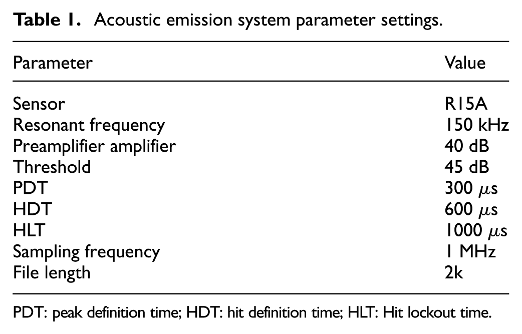
PDT: peak definition time; HDT: hit definition time; HLT: Hit lockout time.

AE signals of high-strength aluminum alloy tensile damage process

AE data were collected during tensile test. Energy, count, amplitude, rise time, peak frequency, and duration were selected as characteristic parameters to study the tensile damage. Figure 4 shows representative experimental curves of sample 1.

Figure 4.

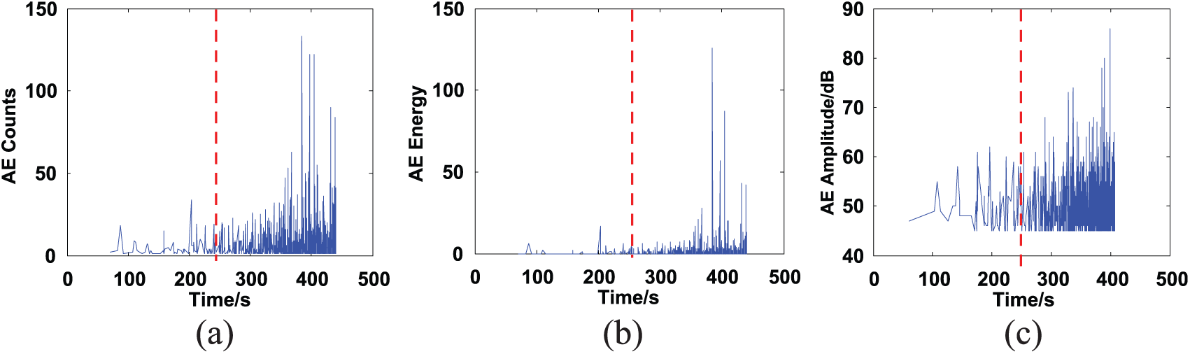
The AE signal features of thermocouple 1: (a) counts, (b) energy, and (c) amplitude.

The transition point from elastic stage to yield stage is the failure point of the tensile process.¹³ Hence, the tensile process can be divided into two stages according to the tensile curve, that is, the elastic region is the safe stage and plastic deformation is the alert stage. Accordingly, the AE data in safe stage are short due to the short elastic nature of the material. It has been shown in Ai et al.¹³ that the AE signal boundary between elastic stage and plastic stage is not clear, and the AE signals of different samples have the same tendency but significantly different values. Therefore, it is difficult to establish a consistent model with the raw data from the AE equipment. The statistically different dispersion of features such as voids in the material is the cause of the above phenomenon. Besides, Figure 4 shows that tensile damage is a relatively short-termed process and that the volatility of the AE data is relatively high. Therefore, a new method for dealing with the AE signal and predicting the residual life of the material’s tensile response is needed.

Results and discussion

Initial life prediction model

Analysis of the characterization parameter

The AE signal data collected during the tensile tests were built into characteristic parameter set series, namely, C(t) for time t

C (1), C (2), C (3), \dots, C (t), \dots

(1)

where

C (t) = [c_{1} (t) c_{2} (t) c_{3} (t) c_{4} (t) c_{5} (t) c_{6} (t)]

(2)

where $c_{1} (t) - c_{6} (t)$ are the AE count, energy, amplitude, rise time, duration, and peak-frequency signals at time t, respectively. For each test, the characteristic parameter set is as follows

\begin{matrix} C = {[C (1) C (2) C (3) \dots C (t) \dots]}^{T} = \\ [\begin{matrix} \begin{matrix} c_{1} (1) & c_{2} (1) & c_{3} (1) \\ c_{1} (2) & c_{2} (2) & c_{3} (2) \\ ⋮ & ⋮ & ⋮ \end{matrix} \begin{matrix} c_{4} (1) & c_{5} (1) & c_{6} (1) \\ c_{4} (2) & c_{5} (2) & c_{6} (2) \\ ⋮ & ⋮ & ⋮ \end{matrix} \\ \begin{matrix} c_{1} (t) & c_{2} (t) & c_{3} (t) \\ ⋮ & ⋮ & ⋮ \end{matrix} \begin{matrix} c_{4} (t) & c_{5} (t) & c_{6} (t) \\ ⋮ & ⋮ & ⋮ \end{matrix} \end{matrix}] = \end{matrix}

(3)

\begin{matrix} [c_{1} c_{2} c_{3} c_{4} c_{5} c_{6}] \\ c_{i} = {[c_{i} (1) c_{i} (2) \dots c_{i} (t) \dots]}^{T}, i = 1, 2, 3, 4, 5, 6 \end{matrix}

(4)

In theory, the correlation coefficient series for the same sample should be larger at beginning and fluctuate with each new data acquired. Finally, after a large amount of data has been collected, the correlation coefficients should gradually stabilize. The count, energy, and amplitude have the same tendency, while the rise time reflects the response speed. Furthermore, a given parameter of AE signal would initially vary significantly with rise time and subsequently dampen. Figure 5 shows the results of the correlation coefficients between the AE signals.

Figure 5.

The results of the correlation coefficients between AE signals.

It can be seen that the correlation coefficients of rise time versus peak frequency are not consistent with the other curves, which is governed by the characteristics of the peak frequency signal, as shown in Figure 7. The count, energy, duration, and amplitude versus rise time correlation coefficients are very high and have a value of nearly ~1. The curves of rise time versus count, rise time versus energy, rise time versus duration, and rise time versus amplitude show early fluctuation, decreasing to a steady-state value. The demarcation points of the tensile process from elastic stage to yield stage are in oscillation decline phase of the curves. However, near each demarcation point, the correlation coefficient has a vibration, which is mainly due to the fast nature of the tensile test. Hence, the time from elastic stage to yield stage is at a relatively shorter time. In addition, with the dispersion of the casting material, the median values of the above correlation coefficients were chosen in order to reduce the fluctuation of the correlation coefficients in this study.

Compared with the average value of the time series, the median value is relatively more concentrated; hence, it was selected for the correlation coefficient of the median time series, C_risemedian

C_{risemedian} = {[C_{risemedian} (1) C_{risemedian} (2) \dots C_{risemedian} (t) \dots]}^{T}

(5)

C_{rise me dian} (t) = median (c_{corr}^{j} (t)), j = 2, 3, 4, 5

(6)

c_{corr}^{j} (t) = ρ (c_{i} (t), c_{j} (t)), i = 1, j =, 2, 3, 4, 5

(7)

ρ (c_{i} (t), c_{j} (t)) = \frac{E [(c_{i}^{t} - E (c_{i}^{t})) (c_{j}^{t} - E (c_{j}^{t}))]}{D (c_{i}) D (c_{j})}

(8)

c_{i}^{t} = {[c_{i} (1) c_{i} (2) \dots c_{i} (t)]}^{T}, c_{j}^{t} = {[c_{j} (1) c_{j} (2) \dots c_{j} (t)]}^{T}

(9)

The C_risemedian of a selected tensile test is shown in Figure 6.

Figure 6.

The C_risemedian of tensile test.

It can be seen that the C_risemedian time series is initially volatile tending to a more steady value with time. The transition point of elastic stage to yield stage was at the oscillatory decreased stage, and the values of the samples at the demarcation point are relatively closed. Therefore, if the curve of the fluctuation stage before the oscillatory decreased stage can be removed, it is possible to characterize the tensile process with the AE parameters. Figure 7 shows the peak frequency of an AE signal.

Figure 7.

The peak frequency of AE signals.

It can be seen from Figure 7 that the peak frequency signal has a relatively high value just before the transition point and exhibits two relatively concentrated values: the high value and low value of different sizes. So, the peak frequency signal of the first time can be considered as the trigger signal for damage identification and life prediction during tension. According to the 16 tests, the values of the peak frequency are all higher than 155, which can be used to judge the high value of peak frequency.

To establish life prediction model

The values of C_risemedian at the transition point of the 16 tests are concentrated. C_Tpoint has been defined as the criterion for tensile damage, which is a statistical result of C_risemedian at the transition point. 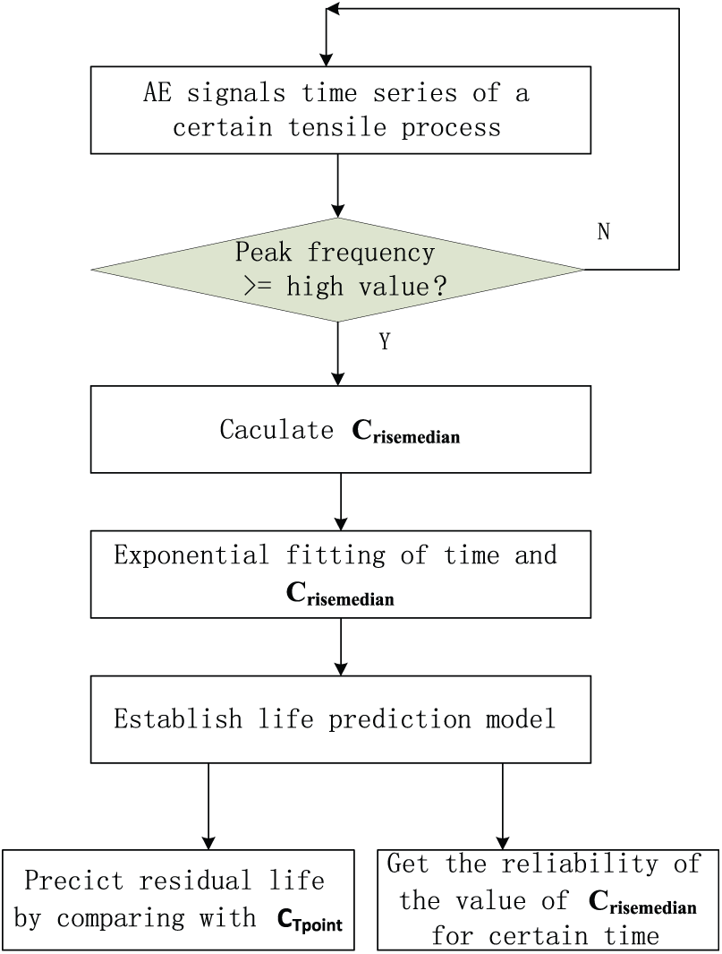So, C_Tpoint is a value with a certain distribution and reflects the distribution of the C_risemedian value at the transition point 15 of the 16 tensile test data that have been used for calculating the C_Tpoint and its probability distribution, $F_{T} C_{Tpoint}$ , at each time, while the remaining test data are used to establish life prediction model for the tensile test. For that data, the continuous AE signal is received under monitoring, and the process before the first high value of peak frequency is considered as the safety stage. Once the peak value is triggered, the value of C_risemedian is continuously redefined by the newly arriving data. The whole C_risemedian time series is then used for exponential fitting to establish the life prediction model. The model can be compared with C_Tpoint to predict the residual life at the transition point or to estimate the reliability of certain time. The detailed algorithm flow is shown in Figure 8.

Figure 8.

The detailed algorithm flow of the initial life prediction model.

The exponential curve fitting uses the form of f(x) = a*exp (b*x), where a and b are the fitting function parameters. After the peak frequency has been triggered successfully, the data 10 s before the transition point were used for the curve fitting. Then, the fitting curve can be compared with the original C_risemedian time series.

Figure 9 shows the prediction result and the real value, and the dotted lines correspond to the transition points of the prediction result and the real value. More prediction result and fitting information are shown in Table 2.

Figure 9.

The comparison of prediction result and real-time series C_risemedian.

Table 2.

The prediction result of initial tensile life prediction model.

No.	Mean ofC_Tpoint	Varianceof C_Tpoint	Time of transitionpoint (s)	Prediction time oftransition point (s)	Error of the predictionresult (s)
1	0.4696	0.1693	250.3	371	−120.7
2	0.4725	0.1705	271	276.9	−5.9
3	0.4782	0.1704	305.2	280.8	24.4
4	0.4702	0.1697	217.8	270.2	−52.4
5	0.4893	0.1605	223.5	204.4	19.1
6	0.4912	0.1575	376.5	180.8	195.7
7	0.4767	0.1708	93.4	66.9	26.5
8	0.4443	0.1138	22.8	51.4	−28.6
9	0.4905	0.1586	922.1	901.1	21
10	0.4666	0.1672	235.2	255.1	−19.9
11	0.4771	0.1707	263.6	145	118.6
12	0.4734	0.1707	191.3	176.4	14.9
13	0.4765	0.1708	152.6	140	12.6
14	0.4726	0.1706	226.1	230	−3.9
15	0.4788	0.1702	820.2	606.8	213.4
16	0.4749	0.1709	554.7	436	118.7

It can be seen from Table 2 that the prediction results obtained by conventional exponential curve fitting is not ideal. Most errors of the samples are within 30 s, some prediction results are after the transition point, and some results of the samples have a large deviation. Careful analysis revealed that these problems are mainly caused by three reasons: first, the sample data near the transition point fluctuates and decreases, which creates errors in the fitting result; second, the data of some samples for fitting are so little to the inaccuracy of the result; finally, because of the dispersion of the material, the values of C_risemedian time series near the transition point are overall either higher or lower than the C_Tpoint value, which creates the large deviations. It is therefore necessary to come up with a targeted solution for improving the accuracy of life prediction model.

Automatic optimization for the life prediction model

Automatic optimization algorithm for few and imbalanced data

Based on the life prediction results of the tensile damage and the analysis of the reasons of the larger deviations, an adaptive optimization method of existing models has been used as follows.

First, for the oscillation problem in the decreased process of the sample data, the smoothing method has been used to avoid increasing adjacent elements and reducing the prediction accuracy of the life prediction model. The moving average method is used to smooth the sample data which are required to be fitted by exponential fitting, and the result will be used as the input for the subsequent interpolation and standard deviation compensation.

Second, for the problem of few samples and the imbalanced data, when the adjacent AE signal time interval is greater than 3 s, the interpolation method has been used for increasing the sample size. The time series trend of C_risemedian near the demarcation point is oscillatory downward. Therefore, in the relatively small interval of two adjacent elements of the C_risemedian time series, it can be considered as a linear relationship. So, the linear interpolation method can be used for interpolation, and the difference interval is 1 s:

if $T (t) - T (t - 1) \geq 3 %$ when the time interval of AE signal is greater than 3 s $T' (t) = T (t - 1) : 1 : T (t) C'_{riseintermedian} = interp 1 ({[T (t - 1) T (t)]}^{T},$

${[C_{risemedian} (t - 1) C_{risemedian} (t)]}^{T}, T^{'} (t)) %$

to run with the interpolation method to increasing the sample size

end

Third, it can be seen from Table 3 that the normal distribution variance of the material failure criteria C_Tpoint is very low, where $σ$ is nearly 0.16 and $μ$ is ∼0.47. The values of the C_risemedian time series at the transition point of certain samples are overall either higher or lower than the C_Tpoint value, resulting in the prediction deviation. So, the standard deviation compensation method of C_risemedian has been used to adjust the C_risemedian result of the life prediction model. When several output $C'_{risemedian}$ values of the interpolation method are larger than $σ$ compared with the mean of the C_Tpoint, the standard deviation compensation method will be used for $C'_{risemedian}$ , which is $Δ = \pm σ$

If $| {C'}_{risemedian} (t) - μ_{Tpoint} | \geq σ_{Tpoint}$ and $| {C'}_{risemedian} (t - 1) - μ_{Tpoint} | \geq σ_{Tpoint}$ and $| {C'}_{risemedian} (t - 2) - μ_{Tpoint} | \geq σ_{Tpoint}$

% when certain sample value are overall higher or lower than sample mean value

If $C'_{risemedian} (t) - μ_{Tpoint} > 0$

$γ = - 1 %$ the certain sample value is overall higher than sample mean value

else $γ = 1 %$ the certain sample value is overall lower than sample mean value

end

${C^{″}}_{risemedian} (t) = {C^{'}}_{risemedian} (t) + γ σ_{Tpoint} %$ to make the standard deviation compensation

end

Table 3.

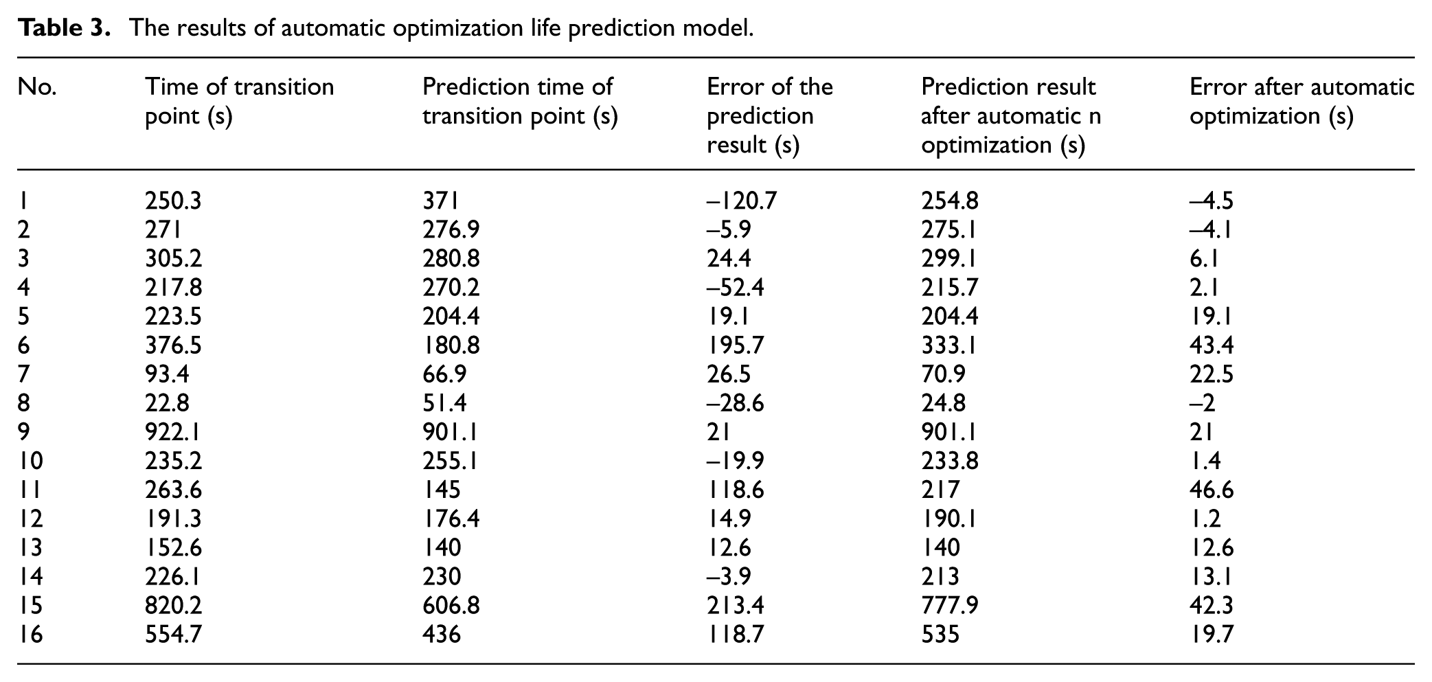
The results of automatic optimization life prediction model.

No.	Time of transitionpoint (s)	Prediction time oftransition point (s)	Error of thepredictionresult (s)	Prediction resultafter automatic noptimization (s)	Error after automaticoptimization (s)
1	250.3	371	−120.7	254.8	−4.5
2	271	276.9	−5.9	275.1	−4.1
3	305.2	280.8	24.4	299.1	6.1
4	217.8	270.2	−52.4	215.7	2.1
5	223.5	204.4	19.1	204.4	19.1
6	376.5	180.8	195.7	333.1	43.4
7	93.4	66.9	26.5	70.9	22.5
8	22.8	51.4	−28.6	24.8	−2
9	922.1	901.1	21	901.1	21
10	235.2	255.1	−19.9	233.8	1.4
11	263.6	145	118.6	217	46.6
12	191.3	176.4	14.9	190.1	1.2
13	152.6	140	12.6	140	12.6
14	226.1	230	−3.9	213	13.1
15	820.2	606.8	213.4	777.9	42.3
16	554.7	436	118.7	535	19.7

Fourth, after a tensile process, the new failure data are used to modify the failure criteria of the characteristic parameters as well as to modify the normal probability distribution of the original failure criteria.

The detailed algorithm flow of automatic optimization life prediction model for the gearbox shell tensile damage is shown in Figure 10.

Figure 10.

The detailed algorithm flow of automatic optimization life prediction model for gearbox shell tensile damage process.

Automatic optimization result and analysis

The results of automatic optimization life prediction model are shown in Table 3.

It can be seen from Table 3 and Figure 11 that the predictive accuracy of automatic optimization life prediction model significantly improved, which is due to the smoothing, interpolation, and overall compensation method for the data. Some results of certain samples have not improved, which is because the automatic optimization method proposed in this study is not in all cases to be adaptively optimized and can only optimize situations such as large oscillation of two adjacent elements, lager time intervals of two adjacent elements, and characterization parameters needing overall compensation.

Figure 11.

The comparison of life prediction model before and after the automatic optimization.

It can be seen from the result of the automatic optimization life prediction model that the life prediction errors are controlled within 50 s, and most of the test data error is less than 20 s. According to the acceleration test design relationship, 20 s error roughly corresponds to 1400 km or 6 h in real operation situation. There is also the prediction result which is after the presence of the real time of the demarcation point, but compared with the whole process of tensile damage, the material is in the plastic stage of the tensile damage process in the lag time of prediction and have not yet entered the fracture stage. So, it will not bring the final burst failure and accident disaster.

Conclusion

In this article, the tensile damage accumulation of a high-speed train gearbox shell material has been studied. For the short tensile process leading to significant damage, a real-time and non-destructive detection method has been used to monitor the tensile damage accumulation and to predict the residual life of the material. For cases where the data of the tensile process are not balanced and the volume of the data at the demarcation point from safety stage to alert stage is low, an automatic algorithm has been proposed to deal with the problem. The algorithm deals with the data fluctuations, imbalances, and large intervals by smooth, interpolation, compensation, and other methods. Based on the above techniques, the automatic optimization life prediction model for material tensile process has been established. The life prediction errors are controlled within 50 s, and the majority of errors are less than 20 s. The test is accelerated, and when compared with the real operation situation, there are about 6 h left for evacuation of passengers and handling failures of the high-speed train.

Footnotes

Handling Editor: Wenbing Zhao

Declaration of conflicting interests

The author(s) declared no potential conflicts of interest with respect to the research, authorship, and/or publication of this article.

Funding

The author(s) disclosed receipt of the following financial support for the research, authorship, and/or publication of this article: The financial support for this study was provided by the National Natural Science Foundation of China (Grant No. 61273205), the Fundamental Research Funds for the Central Universities of China (Grant No. FRF-SD-12-028A), and the 111 Project (Grant No. B12012).

ORCID iD

Yibo Ai

References

Qin

Chen

et al . Axisymmetric numerical simulation of plastic damage in aluminum alloy induced by long pulsed laser. Opt Laser Eng 2010; 48: 361–367.

Darras

Abed

Pervaiz

et al . Analysis of damage in 5083 aluminum alloy deformed at different strain rates Basil. Mat Sci Eng A: Struct 2013; 568: 143–149.

Shui

Wang

Gong

Evaluation of plastic damage for metallic materials under tensile load using nonlinear longitudinal waves. NDT&E Int 2013; 55: 1–8.

Wang

ZG.

Forming limit stress diagram prediction of aluminum alloy 5052 based on GTN model parameters determined by in situ tensile test. Chinese J Aeronaut 2011; 24: 378–386.

Zhu

Mobasher

Rajan

et al . Characterization of dynamic tensile testing using aluminum Alloy 6061-T6 at intermediate strain rates. J Eng Mech 2011; 137(10): 669–679.

Luo

Haya

Inaba

et al . Damage evaluation of railway structures by using train-induced AE. Constr Build Mater 2004; 18: 215–223.

Jalaj

Sony

Mukhopadhyay

et al . Acoustic emission during tensile deformation of smooth and notched specimens of near alpha titanium alloy. Res Nondestruct Eval 2012; 23: 17–31.

Haneef

Lahiri

Bagavathiappan

et al . Study of the tensile behavior of AISI type 316 stainless steel using acoustic emission and infrared thermography techniques. J Mater Res Technol 2015; 137: 1–13.

Chen

Choi

JH.

Acoustic emission study of fatigue cracks in materials used for AVLB. J Nondestruct Eval 2004; 23: 133–151.

10.

Johnson

Waveform based clustering and classification of AE transients in composite laminates using principal component analysis. NDT&E Int 2002; 35: 367–376.

11.

Lomov

Karahan

Bogdanovich

et al . Monitoring of acoustic emission damage during tensile loading of 3D woven carbon/epoxy composites. Text Res J 2014; 84(13): 1373–1384.

12.

Máthis

Prchal

Novotný

et al . Acoustic emission monitoring of slow strain rate tensile tests of 304L stainless steel in supercritical water environment. Corros Sci 2011; 63: 59–63.

13.

Sun

Que

et al . Investigation of material performance degradation for high-strength aluminum alloy using acoustic emission method. Metals 2015; 5: 228–238.

14.

Zhang

Yang

et al . Damage characterization and recognition of aluminum alloys based on acoustic emission signal. J Univ Sci Technol Beijing 2013; 35: 626–633.

Life prediction of the tensile damage progress for high-speed train gearbox shell based on acoustic emission sensor and an automatic optimization method