Multiple underwater target positioning with optimally placed acoustic surface sensor networks

Abstract

In an increasing number of scientific and commercial mission scenarios at sea, it is required to simultaneously localize a group of underwater targets. The latter may include moored systems, autonomous vehicles, and even human divers. For reasons that have to do with the unavailability of Global Positioning System underwater, cost reduction, and simplicity of operation, there is currently a surge of interest in the development of range-based multiple target localization systems that rely on the computation of the distances between the targets and a number of sensor nodes deployed at the ocean surface, equipped with acoustic range measuring devices. In the case of a single target, there is a wealth of literature on the problem of optimal acoustic sensor placement to maximize the information available for target localization using trilateration methods. In the case of multiple targets, however, the literature is scarce. Motivated by these considerations, we address the problem of optimal sensor placement for multiple underwater target positioning. In this setup, we are naturally led to a multiple objective optimization problem, the solution of which allows for the analysis of the trade-offs involved in the localization of the targets simultaneously. To this end, we resort to tools from estimation theory and multi-objective optimization. For each target, the function to be minimized (by proper choice of the sensor configuration) is related to the determinant of the corresponding Fisher information matrix, which yields information on the minimum possible covariance of the error with which the position of the target can be estimated using any non-biased estimator. To deal with the fact that more than one target is involved, we exploit the concept of multiple objective Pareto-optimal solutions to characterize the best possible accuracy with which each of the targets can be positioned, given constraints on the desired positioning accuracy of the other targets. Simulation examples illustrate how, for a three-sensor network and two targets, it is possible to define an optimal sensor configuration that yields large positioning accuracy for both targets simultaneously, using convex optimization tools. When more than two targets are involved, however, more than three sensors are required to exploit an adequate trade-off of the accuracy with which each target can be positioned by resorting to non-convex and Pareto-optimization tools. We show how in this case the optimal sensor configurations depend on the Pareto weights assigned to each of the targets, as well as on the number of sensors, the number of targets, and the uncertainty with which the positions of the targets are known a priori.

Introduction

Fast-paced advances in miniaturized sensors, energy efficient actuators, and low-cost embedded computer systems are steadily impacting the development of autonomous, remotely operated, and hybrid marine vehicles and making them ubiquitous in many scientific and commercial applications. Examples of the latter include marine habitat mapping, geotechnical surveying, inspection of critical infrastructures in the offshore energy and aquaculture industries, archaeologic surveying, and support to human diver operations. Current technology is also enabling the operation of multiple marine vehicles working in cooperation by exploiting the availability of increasingly sophisticated acoustic and optical underwater communication networks. This trend is clearly visible in applications where a group of vehicles carrying complementary resources and working cooperatively have the potential to outperform a single and bulky vehicle in terms of cost, reliability, and mission efficiency. Multiple vehicle operations are also becoming increasingly important in challenging applications where a group of underwater vehicles work in cooperation with mobile or fixed nodes at the surface, capable of giving navigational support to the submerged units and tracking their motion, thus dispensing with the need for the constant presence of overly expensive support ships.

One of the most important tasks enabling multiple vehicle operations is vehicle positioning. In its most general form, proper execution of this task will enable each vehicle in a group of vehicles to know its position and possibly that of a number of neighbors accurately via a communications network. In aerial and terrestrial applications, it is common practice to do vehicle positioning using GPS (Global Positioning System). This system has a wide coverage and provides navigation data to multiple vehicles simultaneously with low power requirements; moreover, its signals do not interfere significantly with the ecosystem. There are, however, many situations in which GPS is not an option because of the absence of electromagnetic signals carrying position-related information. Such is the case in GPS denied environments on land (e.g. tunnels, caves, and complex infrastructures) and underwater. The latter will be the focus of the present article. In these circumstances, positioning and communications rely heavily on the use of acoustic signals. In what concerns acoustic-based positioning, the systems used are drastically different from GPS, have a reduced area coverage (with a maximum of a few kilometers), and are required to withstand the harsh conditions imposed by the water medium (e.g. multipath and Doppler shift effects, latency, and temporary masking of acoustic signals). In spite of these difficulties, however, acoustic-based positioning systems play an increasingly important role in the development of operational systems at sea, in an attempt to reduce the costs that come from using more classical solutions such as inertial-based navigation. It is for this reason that in this article we focus on acoustic-based positioning.

In the above context, the systems available for underwater positioning are quite diverse and suited for a number of different tasks, but they are mainly based on measuring the ranges (distance) or bearings (azimuth and elevation (AE) angles) between the target or targets to be localized and the acoustic sensors placed at known positions. The most important commercial systems are Long-Baseline (LBL) systems, Short-Baseline (SBL) systems, Ultra Short-Baseline (USBL) systems, and the GIB (GPS Intelligent Buoys) systems. For a review on these systems, the reader is referred to Moreno-Salinas et al.’s ¹ study of Section 2. In the present work, motivated by the desire to develop cost-effective solutions to the problem of underwater target positioning, we address the problem of multiple target estimation based on measurements of the ranges between the targets and acoustic sensors at the sea surface. A key issue is that of determining the optimal placement of the sensors so as to maximize the information available for multiple target positioning. We restrict ourselves at this stage to the scenarios where the targets are fixed. This should be viewed as a first step in the derivation of advanced algorithms for multiple mobile target positioning, the principles of which have been exposed in Moreno-Salinas et al., ² which describes an integrated motion planning, control, and estimation architecture for acoustic-based target position estimation.

Optimal sensor placement for single target localization

Interesting results in the area of optimal sensor placement go back to the work of Abel, ³ where the Cramer–Rao Bound (CRB) is used as an indicator of the accuracy of source position estimation, Levanon ⁴ where the lowest possible geometric dilution of precision (GDOP) is computed to determine the optimal location of sensors in two-dimensions (2D), and Aranda et al. ⁵ where a new closed form expression of the Fisher information matrix (FIM) determinant is computed for 2D and 3D (three-dimensional) scenarios and the global optimal is characterized for the 2D case. Important work in this field includes also Yang and Scheuing, ⁶ Yang, ⁷ Neering et al., ⁸ Jourdan and Roy, ⁹ Bishop et al., ¹⁰ Isaacs et al., ¹¹ Dogancay and Hmam, ¹² and Lui and So. ¹³ In general, the above works search for the conditions that optimize some indicator based on the FIM or the CRB to define the optimal sensor positions in 2D scenarios. For a detailed review on these works, the reader is referred to Moreno-Salinas et al. ¹ and the references therein. Some other interesting works that deal with the problem of optimal sensor placement for practical application problems are Zayats and Steinberg, ¹⁴ Mohan Rao and Anandakumar, ¹⁵ or Chakrabarty et al. ¹⁶ In Zayats and Steinberg, ¹⁴ seismic sensor network configurations are derived to maximize the precision with which the location of earthquakes is determined. The maximization of the logarithm of the FIM determinant is used as an optimality criteria. In Mohan Rao and Anandakumar, ¹⁵ a swarm of sensors is employed in a health monitoring system for structures such as bridges, where the optimal placement of the sensors is defined using a swarm intelligence technique called Particle Swarm Optimization (PSO), and in Chakrabarty et al., ¹⁶ a sensor network with a large number of nodes is used for surveillance. Recent work on the problem of optimal sensor placement for single target positioning in the context of autonomous vehicles using the CRB and FIM includes Moreno-Salinas et al., ¹ Perez-Ramirez et al., ¹⁷ Zhao et al., ¹⁸ and Moreno-Salinas et al., ¹⁹ where analytical solutions are shown for single target positioning with range and/or bearings measurements.

Previous work by the authors on the problem of single target localization goes back to Moreno-Salinas et al.^20,21 In Moreno-Salinas et al., ²⁰ an initial solution for the problem of underwater target positioning with range measurements using a surface sensor network was introduced. In Moreno-Salinas et al., ²¹ the study was extended to the situation in which the target position is known with uncertainty. These works were extended for underwater target positioning with AE measurements in Moreno-Salinas et al. ¹ In Moreno-Salinas et al., ¹⁹ an analytical characterization of all possible global optimal solutions for single target positioning in 3D scenarios was provided, considering the realistic situation in which the target position is known with uncertainty. Finally, in Moreno-Salinas et al., ² an integrated motion planning, control, and estimation architecture is developed for a single surface vehicle, which executes sufficiently exciting maneuvers so as to increase the target position estimation accuracy.

Optimal sensor placement for multiple target localization

Based on the previous results, we address the problem of computing the optimal geometric configuration of a surface sensor network that will maximize the range-related information available for multiple target localization in 3D space. We address explicitly the localization problem in 3D using a sensor array located in a finite spatial region (2D) as an interesting application scenario where the sensors are located at the sea surface and the targets to be localized can be placed at any point beneath the surface, although the methodology can be easily extended for an unconstrained sensor network. Furthermore, we incorporate directly into the problem formulation the fact that multiple targets must be localized simultaneously and that the required accuracy for each of the targets may be different. We assume that the range measurements are corrupted by white Gaussian noise with constant covariance. The computation of the target positions may be done, as usual, by resorting to trilateration algorithms.^22–24

Given the above problem framework, the optimal sensor configuration may be computed by analyzing the CRB or FIM for each of the targets. In this sense, the reader is referred to Van Trees ²⁵ for a presentation of this subject in the context of estimation theory. In the problem at hand, the determinants of the FIMs corresponding to the targets are used for the computation of an indicator of the localization performance that is achievable, with a given sensor configuration, for each of the targets involved in the positioning problem. Maximizing this indicator yields the most appropriate sensor formation geometry.

Clearly, there will be trade-offs involved in the precision with which each of the targets can be localized; to study them, we resort to techniques that borrow from estimation theory and Pareto optimization. For the latter, the reader is referred to Khargonekar and Rotea, ²⁶ Cunha and Polak, ²⁷ and Vincent and Grantham. ²⁸ Stated briefly, we avail ourselves of concepts on Pareto optimality and maximize combinations of the logarithms of the determinants of the FIMs for each of the targets in order to compute the Pareto-optimal surface that gives a clear image of the trade-offs involved in the multi-objective optimization problem. We thus obtain a powerful tool to determine the sensor configuration that yields, if possible, a proper trade-off for the accuracy with which the position of the different targets can be computed.

The optimal geometry of the sensor network, that is, the sensor positions, will depend on multiple factors such as the constraints imposed by the task (e.g. the maximum number and type of sensors that can be used, the constraints on the sensor placement), the constraints imposed by the environment (e.g. ambient noise, regions where the sensors cannot be placed, obstacles, etc.), the number of targets and their configuration, the uncertainty on the a priori knowledge on their positions, and the possibly different degrees of precision with which their positions should be estimated. An inadequate sensor configuration may yield large localization errors for some or all of the targets. It is interesting to remark that even though the problem of optimal sensor placement for range-based multiple target localization is of great importance, not many results are available on this topic yet. A representative reference that deals with the problem of multiple target positionining is Sheng and Hu, ²⁹ where a maximum likelihood acoustic source location estimation method for wireless ad hoc sensor networks is used to estimate multiple acoustic source locations with received signal strength (RSS) measurements. To solve the optimization problem of maximum likelihood estimation, two methods are used: a multiresolution search algorithm and an expectation–maximization-like iterative algorithm. The authors show that, for a single target, the sensors must be close to the target and keeping a regular formation around it to obtain good localization accuracy, and how for multiple targets, if the distance between them is large, the accuracy degrades substantially. In Cheng et al., ³⁰ the underwater localization problem is studied in sparse 3D acoustic sensor networks. The authors consider the depth known by depth sensors, so they transform the problem in a 2D localization problem. In Zhou et al., ³¹ the problem of localization in large-scale underwater sensor networks is studied. The authors propose the localization of a first level of vehicles from surface buoys or anchor nodes, and from them, the localization of a second level of nodes that cannot comunicate with the surface buoys. However, they focus on the localization of the latter nodes, considering a perfect localization of the first-level nodes by the surface sensors. They employ an hybrid approach based on a 3D Euclidean distance estimation method and a recursive location estimation method to localize the nodes. In Feng et al., ³² the authors addressed the problem of multiple target localization by exploiting compressive sensing theory. The location of the targets is determined by RSS measurements, using a $l_1$ minimization program. Finally, in the work of Liu et al., ³³ multiple underwater acoustic sources are localized by an antenna array beamforming based on the matched field processing. The problems that matched field processing presents for detecting sources close to each others and the high noise are overcome with a sparse representation of a small number of source positions among a much larger number of potential positions. However, the above references are focused on the localization problem, not on optimal sensor placement for maximizing the estimation accuracy. Exceptions that deal with the problem of optimal sensor configurations include Moreno-Salinas et al. ³⁴ and Rosa, ³⁵ in which this problem is initially studied using convex optimization tools, and Moreno-Salinas et al., ³⁶ where the problem of optimal configurations is studied analytically and numerically for 2D scenarios. In particular, Moreno-Salinas et al. ³⁴ deal with a similar scenario where a surface sensor network is used for multiple underwater target localization. However, in Moreno-Salinas et al., ³⁴ it is assumed that the logarithm of the FIM determinant is a concave function, and then, convex optimization tools are employed to define the optimal configurations, namely, a gradient-based optimization algorithm. In addition, although the formulation of the problem is given in a general setup, only the two-target localization problem is studied. In the present work, as an important step forward, we prove that the assumption of concavity of the logarithm of the FIM determinant holds for the case of a three-sensor network but not necessarily for a network with a larger number of sensors. In the latter case, the gradient-based optimization algorithm proposed in Moreno-Salinas et al. ³⁴ could fail in providing an optimal sensor configuration. Thus, non-convex optimization techniques must be employed in the search of optimal sensor placement. In addition, in this article, the problem is generalized for any number of targets and studied in detail for multiple situations of interest that show clearly that some trade-offs must be adopted to define reliable solutions.

We would like to stress that following what is commonly reported in the literature, we start the analysis by addressing the problem of optimal sensor placement given an assumed position for the targets. This assumption is unrealistic, since the positions of the targets are known in advance, but stems from the need to first fully understand the simpler situation where the positions of the targets are known and to characterize the types of solutions obtained for the optimal sensor placement problem. In a practical situation, the positions of the targets are known with uncertainty and this problem must be tackled directly. At this stage, an in-depth understanding of the types of solutions obtained for the ideal case is of the utmost importance to compute an initial guess for the optimal sensor placement algorithm adopted. These issues are rarely discussed in the literature, some examples are Moreno-Salinas et al., ¹ Isaacs et al., ¹¹ and Moreno-Salinas et al. ¹⁹ The organization of the article reflects this circle of ideas, establishing the theoretical tools to address and solve the case when there is uncertainty in the positions of the underwater targets.

The key contributions of the present article are twofold: (a) we fully exploit concepts and techniques from estimation theory and multi-objective optimization to obtain a numerical solution to the optimal sensor configuration problem for multiple targets in 3D space, and (b) in striking contrast to what is customary in the literature, we analyze the problem when the target positions are described by density probabilistic functions. This allows us to capture the fact that the target positions are always known with uncertainty.

The article is organized as follows: In the “Problem statement and notation” section, the notation used along the work and the problem formulation are presented. The FIM is explicitly computed and the Pareto optimality is described. In the “Optimal configuration of a three-sensor network” section, the problem of target positioning using a three-sensor network is studied. In this case, the concavity of the indicator can be demonstrated analytically, supporting the use of scalarization and convex optimization techniques to define the optimal sensor placement. In the “Extension to n sensors” section, the optimal sensor placement computation is extended to a generic $n$ sensor formation. In this case, the concavity of the approach cannot be demonstrated analytically, so we must resort to non-convex optimization techniques. In the “Uncertainty in the target positions” section, the problem where the target positions are known with uncertainty is studied. Finally in the “Conclusion” section, the conclusions are presented.

Problem statement and notation

In this section, we summarize the basic notation and definitions that will be used in the sequel, after which we formulate the problem of multiple underwater target positioning in an estimation-theoretical setting.

The Fisher information matrix

Let $\{I\}$ be an inertial reference frame with unit axis $\{x_I\},\{y_I\},\{z_I\}$ and let $q_k=[q_{\mathrm{kx}},q_{\mathrm{ky}},q_{\mathrm{kz}}{]}^T$ be the position of the $k\mathrm{th}$ target to be positioned in $\{I\}$ , with $k=1,\dots ,m$ , where $m$ is the number of targets involved in the task. Further, denote by $p_i=[p_{\mathrm{ix}},p_{\mathrm{iy}},p_{\mathrm{iz}}{]}^T$ ; $i=1,2,..,n$ , the position of the $i\mathrm{th}$ acoustic ranging sensor, also in $\{I\}$ , with $n$ being the number of sensors used. Let $r_i(q_k)=|q_k-p_i|$ (hereafter $r_{\mathrm{ki}}$ ) be the distance (range) between the $i\mathrm{th}$ sensor and the $k\mathrm{th}$ target, where |·| denotes the Euclidean norm.

We denote by $z_{\mathrm{ik}}$ the measurement of the actual range $r_i(q_k)$ between the $i\mathrm{th}$ sensor and the $k\mathrm{th}$ target, corrupted by additive noise ${\omega }_{\mathrm{ik}}$ . With the above notation, the measurement model adopted is given by

$$z_{\mathrm{ik}}=|q_k-p_i|+{\omega }_{\mathrm{ik}}=r_i\left(q_k\right)+{\omega }_{\mathrm{ik}},$$

(1)

where we assume, for each generic $i\mathrm{th}$ sensor; $i=1,2,..,n$ that the measurement noise ${\omega }_{\mathrm{ik}}$ ; $k=1,2,\dots ,m$ can be modeled as a zero-mean Gaussian process with constant variance ${\sigma }_i^2$ , where the latter is the same for all targets. This comes from the fact that this variance is essentially range independent, even though it may vary from sensor to sensor, as explained below. We further assume that for an arbitrary $k\mathrm{th}$ target, the noise sources ${\omega }_{\mathrm{ik}};i=1,2,\dots ,n$ are independent. In this case, the measurement error vector $[{\omega }_{1k},\dots ,{\omega }_{\mathrm{nk}}{]}^T$ that is formed by considering the $k\mathrm{th}$ target and all sensors is a Gaussian process with probability density function $N(0_n,\Sigma )$ , where $0_n$ is a vector of $n$ zeros and $\Sigma =\mathrm{diag}({\sigma }_i^2,\dots ,{\sigma }_n^2)$ . This notation captures the fact that the sensors may have different accuracies and thus different measurement error variances.

As mentioned above, in the setup adopted, we consider the measurement noise model to be distance independent. This assumption is in line with common assumptions reported in the literature. The reader is referred to Moreno-Salinas et al.’s ¹⁹ study of Section II for a detailed justification of the model adopted.

In what follows, we review the concepts of Cramer–Rao Lower Bound (CRLB) and FIM; see, for example, Van Trees ²⁵ for an introductory exposition. Stated in simple terms, the FIM captures the amount of information that measured data provide about an unknown parameter (or vector of parameters) to be estimated. Under well-known assumptions, the FIM is the inverse of the CRB matrix, which sets a lower bound on the covariance of the parameter estimation error that can possibly be obtained with any unbiased estimator. Thus, “minimizing the CRB” may yield (by proper estimator selection) a decrease of the covariance of the parameter estimation error. We start by recalling the theoretical framework that is commonly adopted to solve the problem of optimal sensor placement for single target positioning. The setup will then be extended to accommodate several targets simultaneously.

Consider a generic target with index $k$ and define, for a set of $n$ sensors located at positions $p_1,p_2,\dots ,p_n$ , the vectors $z_k=[z_{1k},\dots ,z_{\mathrm{nk}}{]}^T$ and $r(q_k)=[r_1(q_k),\dots ,r_n(q_k){]}^T$ of measured and actual ranges between the target and each of the sensors, respectively.

Following by now standard procedures, see, for example, Moreno-Salinas et al. ¹⁹ and the references therein, the FIM corresponding to the problem of range-based target positioning for the $k\mathrm{th}$ target can be computed from the likelihood function ${\mathcal{P}}_k(z_k)$ given by

$${\mathcal{P}}_k\left(z_k\right)=\Omega \exp \{-\frac{1}{2}(z_k-r\left(q_k\right)){\Sigma }^{-1}{(z_k-r\left(q_k\right))}^T\}$$

(2)

where

$$\Omega =\frac{1}{{(2\pi )}^{\frac{n}{2}}|\Sigma {|}^{\frac{1}{2}}}$$

Let $1_n\in {\Re }^{\mathrm{nx}1}$ be a vector of 1s and define the matrix of sensor positions $\overline{p}$ in ${\Re }^{3\mathrm{xn}}$ as $\overline{p}=[p_1,\dots ,p_n]$ . Taking the logarithm of equation (2), computing its derivative with respect to $q_k$ and then its expected value, the FIM for target $k$ is defined as

$$\mathrm{FI}{M}_k=C{\left(\delta \left(r\right)\Sigma \delta \left(r\right)\right)}^{-1}{C}^T$$

(3)

where $C=(q_k{1}_n^T-\overline{p})\in {\Re }^{3\mathrm{xn}}$ and $\delta (·)$ is the operator diag. Expanding equation (3) yields

$$\begin{array}{c}\mathrm{FI}{M}_k=\hfill \\ \multicolumn{1}{c}{\sum _{i=1}^n\left(\begin{array}{ccc}{\left(u_{\mathrm{ik},1}\right)}^2\hfill & \left(u_{\mathrm{ik},2}\right)\left(u_{\mathrm{ik},1}\right)\hfill & \left(u_{\mathrm{ik},3}\right)\left(u_{\mathrm{ik},1}\right)\hfill \\ \multicolumn{1}{c}{\left(u_{\mathrm{ik},1}\right)\left(u_{\mathrm{ik},2}\right)}& {\left(u_{\mathrm{ik},2}\right)}^2\hfill & \left(u_{\mathrm{ik},3}\right)\left(u_{\mathrm{ik},2}\right)\hfill \\ \multicolumn{1}{c}{\left(u_{\mathrm{ik},1}\right)\left(u_{\mathrm{ik},3}\right)}& \left(u_{\mathrm{ik},2}\right)\left(u_{\mathrm{ik},3}\right)\hfill & {\left(u_{\mathrm{ik},3}\right)}^2\hfill \end{array}\right)}\end{array}$$

(4)

where

$$u_{\mathrm{ik}}=\left(\begin{array}{ccc}\frac{\partial \Vert q_k-p_i\Vert }{\partial q_{\mathrm{kx}}}\hfill & \frac{\partial \Vert q_k-p_i\Vert }{\partial q_{\mathrm{ky}}}\hfill & \frac{\partial \Vert q_k-p_i\Vert }{\partial q_{\mathrm{kz}}}\hfill \end{array}\right)/{\sigma }_i.$$

For target positioning purposes, the optimal sensor configuration can now be obtained by optimizing some indicator related to the FIM above. In what follows, motivated by the so-called D-optimum design strategy, ³⁷ we adopt, as an indicator, the determinant of the FIM. Other choices are of course possible. With this indicator, for the target with index $k$ taken in isolation, the objective is to compute

$${\overline{p}}_k^{*}=\arg \underset{\overline{p}}{max}\log \left|\mathrm{FI}{M}_k\right|$$

(5)

where, as is customary, $\log \left|\mathrm{FI}{M}_k\right|$ is used instead of $\left|\mathrm{FI}{M}_k\right|$ for mathematical tractability. Notice, however, that maximizing $\log \left|\mathrm{FI}{M}_k\right|$ or $\left|\mathrm{FI}{M}_k\right|$ yields the same optimal solution.

It is relevant to stress that even in the case of a single target, there are multiple solutions that yield the maximum theoretical determinant of the FIM. Following the analytical procedure detailed in Moreno-Salinas et al., ¹⁹ it is possible to show that all optimal solutions lead to the optimal FIM given by

$$\mathrm{FI}{M}_{\mathrm{opt},k}=\sum _{i=1}^n\left(\begin{array}{ccc}\frac{1}{3{\sigma }_i^2}\hfill & 0\hfill & 0\hfill \\ \multicolumn{1}{c}{0}& \frac{1}{3{\sigma }_i^2}\hfill & 0\hfill \\ \multicolumn{1}{c}{0}& 0\hfill & \frac{1}{3{\sigma }_i^2}\hfill \end{array}\right)$$

(6)

Given equation (6), the optimality conditions that a sensor network must satisfy in order to yield the FIM above are given by

$$\begin{array}{cc}\multicolumn{1}{c}{\sum _{i=1}^n\frac{{(q_{\mathrm{kx}}-p_{\mathrm{ix}})}^2}{{\sigma }_i^2{r}_{\mathrm{ik}}^2}}& =\sum _{i=1}^n\frac{{(q_{\mathrm{ky}}-p_{\mathrm{iy}})}^2}{{\sigma }_i^2{r}_{\mathrm{ik}}^2}=\hfill \\ \multicolumn{1}{c}{}& =\sum _{i=1}^n\frac{{(q_{\mathrm{kz}}-p_{\mathrm{iz}})}^2}{{\sigma }_i^2{r}_{\mathrm{ik}}^2}=\frac{1}{3{\sigma }_i^2}\hfill \end{array}$$

(7)

$$\begin{array}{cc}\multicolumn{1}{c}{\sum _{i=1}^n\frac{(q_{\mathrm{kx}}-p_{\mathrm{ix}})(q_{\mathrm{ky}}-p_{\mathrm{iy}})}{{\sigma }_i^2{r}_{\mathrm{ik}}^2}}& =\sum _{i=1}^n\frac{(q_{\mathrm{kx}}-p_{\mathrm{ix}})(q_{\mathrm{kz}}-p_{\mathrm{iz}})}{{\sigma }_i^2{r}_{\mathrm{ik}}^2}=\hfill \\ \multicolumn{1}{c}{}& =\sum _{i=1}^n\frac{(q_{\mathrm{kz}}-p_{\mathrm{iz}})(q_{\mathrm{ky}}-p_{\mathrm{iy}})}{{\sigma }_i^2{r}_{\mathrm{ik}}^2}=0\hfill \end{array}$$

(8)

where $r_{\mathrm{ik}}=r_i(q_k)$ . These conditions allow for a geometric-like characterization of the solutions where the optimal configurations can be analytically defined given the intersections of well-defined quadratic functions and the orthogonality relations of sines and cosines. For a detailed explanation and demonstration of the corresponding mathematical analysis, and how to define optimal sensor configurations for a single target, the reader is referred to Moreno-Salinas et al. ¹⁹

Multi-objective optimization and Pareto optimality

We now tackle the problem of simultaneous multiple target positioning. The solution proposed builds upon the work described in Moreno-Salinas et al. ¹⁹ but departs considerably from it because we address explicitly the problem of simultaneous target positioning. In this situation, it may be impossible, by proper sensor placement, to maximize the determinants of the FIMs corresponding to all the targets involved, simultaneously. Thus, trade-off solutions must be examined. This issue is studied next. We are interested in the problem of optimal sensor placement for multiple target positioning, so we must resort to a multi-objective optimization strategy. To this end, we avail ourselves of the concept of Pareto optimality introduced below. The presentation follows closely the summary in Khargonekar and Rotea. ²⁶

Let $\mathcal{X}$ be an arbitrary non-empty set and let $f_k:\mathcal{X}\to {\mathcal{R}}_{+}$ ; $k=1,2,\dots ,m$ be $m$ non-negative functionals defined on $\mathcal{X}$ . A point $x^0\in \mathcal{X}$ is said to be Pareto optimal with respect to the vector-valued criterion $f:=(f_1,f_2,\dots ,f_m{)}^T$ if there does not exist $x\in \mathcal{X}$ such that

$$f_k\left(x\right)\ge f_k\left(x^0\right)\mathrm{for\; all}k=1,2,\dots ,m$$

and

$$f_l\left(x\right)>f_l\left(x^0\right)\mathrm{for}\mathrm{some}l\in 1,2,\dots ,m.$$

From the above, it follows that if one wishes to find points $x\in \mathcal{X}$ such that, in some sense, $x$ jointly maximizes all the components of $f$ , then one must examine the Pareto-optimal points. It is interesting to point out that in the literature on economics, a Pareto-optimal outcome is one such that no person can be made better off without having someone else worse off.

When Pareto-optimal solutions exist, in general they are not unique. However, the determination of the Pareto-optimal set for a given multi-objective problem allows for a thorough study of the trade-offs involved in the problem at hand. The next scalarization result in Cunha and Polak ²⁷ is of crucial importance in characterizing this set.

Scalarization result

Suppose that $\mathcal{X}$ is a normed linear space and that each component of $f:=(f_1,f_2,\dots ,f_m{)}^T$ is a concave function on $\mathcal{X}$ . Let

$$\Lambda :=\{\lambda \in {\mathcal{R}}^m:{\lambda }_i\ge 0,{\lambda }_1+{\lambda }_2+\cdots +{\lambda }_m=1\}$$

and, for each $\lambda \in \Lambda$ , consider the scalar-valued optimization problem that consists of computing

$$\sup \{{\lambda }^{T}f\left(x\right):x\in \mathcal{X}\}$$

(9)

Suppose that $x^0\in \mathcal{X}$ is Pareto optimal with respect to the vector-valued criterion $f:=(f_1,f_2,\dots ,f_m{)}^T$ . Then, there exists $\lambda \in \Lambda$ such that $x_0$ is a solution to the scalar optimization problem above. Conversely, given $\lambda \in \Lambda$ , if the scalar optimization problem has at most one solution $x^0\in \mathcal{X}$ , then $x^0$ is Pareto optimal with respect to $f(x)$ . Notice that the function ${\lambda }^{T}f(x):x\in \mathcal{X}$ is concave because it is a non-negative weighted sum of concave functions.

The above result yields a powerful methodology to compute all Pareto-optimal points when each component $f_i$ of $f$ is concave on $\mathcal{X}$ . The set of Pareto-optimal solutions is often called the Pareto front or Pareto boundary. In the present article, the scalar functions $f_i$ are related to the logarithms of the determinants of the FIMs corresponding to each of the targets being localized, that is, $f_i=\log \left|\mathrm{FI}{M}_i\right|$ , where $\mathrm{FI}{M}_i=\mathrm{FI}{M}_i(\overline{p})$ is a function of the sensor placement vector $\overline{p}$ .

The objective is to maximize these functions jointly in a well-defined sense. Formally, this can be done by computing

$${\overline{p}}^{*}\left(\lambda \right)=\arg \underset{\overline{p}}{max}\sum _{i=1}^m{\lambda }_i\log \left|\mathrm{FI}{M}_i\left(\overline{p}\right)\right|$$

(10)

where $\lambda \in \Lambda :=\{\lambda \in {\mathcal{R}}^m:{\lambda }_i\ge 0,{\lambda }_1+{\lambda }_2+\cdots +{\lambda }_m=1\}$ and studying the corresponding Pareto-optimal front. Notice that for each value of $\Lambda$ , the above optimization process yields the corresponding values for the objective functions $f_i=\log \left|\mathrm{FI}{M}_i\right|$ , with $\left|\mathrm{FI}{M}_i\right|=|\mathrm{FI}{M}_i(\Lambda )|$ . In the case of two targets, for example, the corresponding Pareto-optimal front is a $|\mathrm{FI}{M}_2(\Lambda )|$ versus $|\mathrm{FI}{M}_1(\Lambda )|$ curve that captures the trade-offs between the two criteria and allows, for example, to compute that maximum possible value of $\left|\mathrm{FI}{M}_2\right|$ given a desired, achievable lower bound for $\left|\mathrm{FI}{M}_1\right|$ . These considerations can be easily generalized to the case of an arbitrary number of targets, as shown next.

Let $\left|{\mathrm{FIM}}_i^{*}\right|$ denote the optimal (maximum) value of $\left|\mathrm{FI}{M}_i\right|$ , corresponding to the $i\mathrm{th}$ target, achievable with optimal sensor positions specified by ${\overline{p}}_i^{*}$ . In general, there is no choice of suitable sensor positions ${\overline{p}}^{*}$ (same for all targets) that will make simultaneously all $\left|\mathrm{FI}{M}_i\right|$ equal or close to the individually optimal ones $\left|{\mathrm{FIM}}_i^{*}\right|;i=1,2,\dots ,m$ . In fact, this would correspond to the ideal situation where, by proper sensor placement, all targets could be simultaneously localized with accuracies similar to the ones achievable for each individual target, but using the same set of sensors. Failure to achieve this may be due to a number of causes that include the geometry of the multiple target positioning problem and possible hard constraints on sensor placement. As a consequence, trade-off solutions must be examined. For example, one may seek to maximize, by proper choice of sensor positions ${\overline{p}}^{*}$ , the accuracy with which one target can be localized, while keeping the accuracies of the other targets above desired, achievable lower bounds.

From a practical standpoint, the Pareto-related optimization problem posed in equation (10) yields two possible optimal sensor placement strategies that, to some extent, correspond to two different interpretations of the weight $\Lambda$ . The first strategy is a simple consequence of remaining close in spirit to the original objective of characterizing the Pareto-optimal front for the multi-objective problem at hand. Conceptually, one may solve the optimization problem for all values of $\Lambda$ and study the trade-offs involved in optimizing each of the cost functions $f_i=\log \left|\mathrm{FI}{M}_i\right|$ . This is in principle possible to do if one grids the search parameter space described by $\Lambda$ and plots an approximation to the corresponding Pareto-optimal front. The latter is instrumental in capturing the trade-offs involved, thus helping a designer choose a specific point on the Pareto front for the particular problem being solved. Clearly, this task is hard for more than three objective functions, for in this case it may not be simple to visualize the Pareto-optimal front of interest. This is a subject of considerable interest, but one that would lead us away from the core contribution of the present article. Suffice it to say that there are methods to deal with the increased dimensionality of the problem, namely, in what concerns efficient methodologies to compute the bounded Pareto fronts of practical multi-objective optimization problems; see, for example, Mueller-Gritschneder et al. ³⁸ and the references therein. The second strategy consists of viewing $\Lambda$ as a a collection of weights ${\lambda }_i;i=1,2,\dots ,m$ where the appearance of a weight, say ${\lambda }_k$ , that is larger than the other weights captures the fact that the priority is to obtain a very good estimate of the position of the $k\mathrm{th}$ target, possibly in detriment of the accuracy with which the other targets can be positioned. Again, the final choice for a reasonable solution involves repeating the procedure for a number of choices of $\Lambda$ and examining the corresponding solutions and how they meet the performance objectives set forth by an end user.

Optimal configuration of a three-sensor network

If the optimal sensor configuration that maximizes the summation of the logarithms of the FIM determinants is to be computed by exploiting the above explained Pareto-optimal conditions, then it is necessary to show concavity of the log determinant function with respect to the design variables. Notice that this is not necessarily implied by the well-known fact that $f(X)=\log \det (X)$ is a concave function over the space of positive definite matrices denoted $X$ . In fact, no general result on concavity of the above cost function in the design parameters is known for this type of problem.

As a contribution to a rigorous solution of the positioning problem, in the present article, we show that in the case of a network with three sensors the cost function adopted is indeed concave in the design parameters, which allows for an elegant solution to the optimization problem described before. A proof of concavity of the cost function for more than three sensors has eluded us. Therefore, for the general case of $n>3$ , the sensor configurations are computed by resorting to optimization tools that, in spite of lacking the elegance of the methods available for the case where the cost function is concave, are extremely useful to tackle a broader class of problems (see the “Extension to n sensors” section).

Concavity of the cost function for a three-sensor network

In the following analysis, for the sake of convenience, we adopt the notation in Aranda et al. ⁵ and write the FIM determinant as

$$\begin{array}{c}\left|\mathrm{FIM}\right|=\frac{1}{{\sigma }^6}{((\frac{\overrightarrow{r_1}}{|r_1|}\times \frac{\overrightarrow{r_2}}{|r_2|})·\frac{\overrightarrow{r_3}}{|r_3|})}^2=\hfill \\ \multicolumn{1}{c}{=\frac{1}{{\sigma }^6}\stackrel{2}{\sin }\left({\alpha }_{12}\right)\stackrel{2}{\cos }\left({\beta }_{12,3}\right)}\end{array}$$

(11)

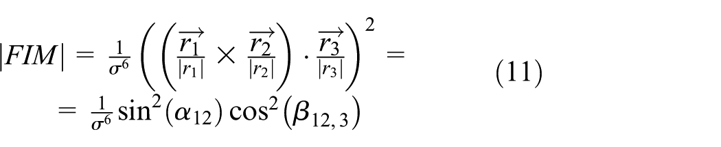
where the meaning of the above variables is clear from Figure 1. In the figure, the red points represent the sensors and the green one denotes the target, placed at the origin of the inertial reference frame $\{I\}$ . Furthermore, ${\alpha }_{12}$ is the angle formed between range vector 1 ( $\overrightarrow{r_1}$ ) and range vector 2 ( $\overrightarrow{r_2}$ ), and ${\beta }_{12,3}$ is the angle formed by range vector 3 ( $\overrightarrow{r_3}$ ) and the vector perpendicular to the plane defined by range vectors 1 and 2 ( $\overrightarrow{r_1}\times \overrightarrow{r_2}$ ).

Figure 1.

Target localization setup with three sensors $p_1$ , $p_2$ , and $p_3$ (red points), and a single target placed at the origin of the inertial reference frame (green point).

Without loss of generality, we assumed for clarity of exposition that the error covariance $\sigma$ in equation (11) is the same for the three sensors. Clearly, in this case, an optimal sensor configuration does not depend on the distance between the target and the sensors and is solely determined by the angles that the range vectors form among them. We may therefore assume that the range vectors $\overrightarrow{r_1}$ and $\overrightarrow{r_2}$ corresponding to sensors 1 and 2, respectively, are in a fixed arbitrary plane containing the origin.

Notice how with the formulation in equation (11) the design parameters in the optimization process are the angles ${\alpha }_{12}$ and ${\beta }_{12,3}$ , and not the positions of the sensors. This is very convenient when seeking a solution to the optimal sensor positioning problem. We now demonstrate the concavity of $\log |\mathrm{FIM}|$ by computing the second derivatives of the logarithm of equation (11) with respect to the angles ${\alpha }_{12}$ and ${\beta }_{12,3}$ and showing that the Hessian matrix of the above cost function is positive definite. The computation of the cost function $\log |\mathrm{FIM}|$ requires that the matrix $\mathrm{FIM}$ be positive definite. For this reason, the domain of the logarithm of equation (11) cannot contain values of ${\alpha }_{12}$ and ${\beta }_{12,3}$ for which the determinant becomes zero, that is, the sensors and the target cannot lie in the same plane. Therefore, ${\alpha }_{12}\in ]0,\pi [$ or ${\alpha }_{12}\in ]\pi ,2\pi [$ , and ${\beta }_{12,3}\in ]0,\pi [$ or ${\beta }_{12,3}\in ]\pi ,2\pi [$ . For all combinations of the above domains, the solutions are equivalent and define the same sensor formation simply by rotating them through an appropriate angle.

Straightforward computations show that the Jacobian matrix of the above cost function can be written as

$$\nabla \log |\mathrm{FIM}|=\left[\begin{array}{c}\frac{\partial \log |\mathrm{FIM}|}{\partial {\alpha }_{12}}\hfill \\ \multicolumn{1}{c}{\frac{\partial \log |\mathrm{FIM}|}{\partial {\beta }_{12,3}}}\end{array}\right]=\left[\begin{array}{c}\frac{2\cos \left({\alpha }_{12}\right)}{\sin \left({\alpha }_{12}\right)}\hfill \\ \multicolumn{1}{c}{\frac{-2\sin \left({\beta }_{12,3}\right)}{\cos \left({\beta }_{12,3}\right)}}\end{array}\right]$$

(12)

from which it follows that the corresponding Hessian matrix is given by

$$\begin{array}{c}{\mathcal{H}}_{\log |\mathrm{FIM}|}=\left[\begin{array}{cc}\frac{{\partial }^2\log |\mathrm{FIM}|}{\partial {\alpha }_{12}^2}\hfill & \frac{{\partial }^2\log |\mathrm{FIM}|}{\partial {\alpha }_{12}\partial {\beta }_{12,3}}\hfill \\ \multicolumn{1}{c}{\frac{{\partial }^2\log |\mathrm{FIM}|}{\partial {\beta }_{12,3}\partial {\alpha }_{12}}}& \frac{{\partial }^2\log |\mathrm{FIM}|}{\partial {\beta }_{12,3}^2}\hfill \end{array}\right]=\hfill \\ \multicolumn{1}{c}{=\left[\begin{array}{cc}\frac{-2}{\stackrel{2}{\sin }\left({\alpha }_{12}\right)}\hfill & 0\hfill \\ \multicolumn{1}{c}{0}& \frac{-2}{\stackrel{2}{\cos }\left({\beta }_{12,3}\right)}\hfill \end{array}\right]}\end{array}$$

(13)

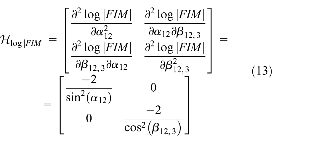
Because in equation (13) the principal minor ${\mathcal{H}}_{\log |\mathrm{FIM}|}(1,1)<0$ and $|{\mathcal{H}}_{\log |\mathrm{FIM}|}|>0$ , it follows that the Hessian matrix (equation (13)) is definite negative and therefore the logarithm of equation (11) is a concave function of its arguments. This justifies the use of Pareto-optimal-related design tools to quantify the trade-offs involved in the computation of optimal sensor placement solutions.

Examples of optimal solutions for multiple target positioning with three sensors

This section contains two examples of the computation of optimal sensor configurations for multiple target positioning, with the number of sensors restricted to 3. Because in this case the cost function adopted is concave, a gradient descent method may be used to compute a global solution to the problem.

The two examples deal with two targets and four targets, respectively. In both examples, the sensors are required to lie inside a square of $600\mathrm{m}\times 600\mathrm{m}$ with its center aligned vertically with the origin of the inertial coordinated frame $\{I\}$ . In each of the examples, the covariance of the range measurement errors is set to ${\sigma }^2=0.01{\mathrm{m}}^2$ for all sensors for simplicity reasons, although the procedure would be identical if different covariances were assigned to each of the sensors. The target depths are set to $50\mathrm{m}$ . It is important to remark that in all the examples reported in the present article, for the sake of clarity and without loss of generality, the targets are considered to be placed in the same plane to allow for a simple graphical representation and a quick comparison of the results obtained, namely, in what concerns the minimum possible variance of the error inherent to the estimation of the position of each target.

We recall that the article aims to study the accuracy with which a number m of fixed underwater targets can be positioned using a number n of range measuring devices. This is done by resorting to estimation-theoretical tools, which afford us the means to compute the minimum possible accuracy with which each target can be positioned using an unbiased estimator. As such, the article does not tackle the problem of target position estimation, for which many solutions are available in the literature. Consequently, we never deal with real or even simulated range data. The only data involved in the simulations are (a) target positions (with or without uncertainty), (b) sensor positions (to be determined by our sensor placement algorithms), and (c) Pareto weights that capture the relative importance attached to each of the targets in terms of desired positioning accuracy. These data (simulation parameters) aim to show different situations of interest where the number and location of the targets, the number of sensors, and Pareto weights impact directly on the accuracy with which each of the target positions can be estimated.

Example 1

In this first example, the distance between the two targets is $100\mathrm{m}$ and they are placed over the $x_I$ axis. Using the theoretical framework described before, the Pareto front corresponding to this scenario was obtained numerically computing, for a sufficiently large number of uniformly distributed values of ${\lambda }_1\in [0,1]$ , the global maximum of ${\lambda }_1{f}_1+{\lambda }_2{f}_2={\lambda }_1{f}_1+(1-{\lambda }_1)f_2$ as a function of the design parameters, with $f_i=\log \left|\mathrm{FI}{M}_i\right|;i=1,2$ , and using a gradient descent algorithm with the Armijo rule ³⁹ (see Figure 2). The figure shows clearly that in this case, no matter what the value of ${\lambda }_1$ is, the corresponding optimal values of $\left|\mathrm{FI}{M}_i\right|;i=1,2$ are quite close to the optimal value obtainable for each target individually, given by $|\mathrm{FIM}|=n^3/(3^3{\sigma }^6)=1\times {10}^6$ , where $n$ is the number of sensors. For this reason, in what follows we fix ${\lambda }_1={\lambda }_2=0.5$ , that is, the Pareto weights are equal to $0.5$ .

Figure 2.

Pareto-optimal front for two targets and three sensors.

For this choice of Pareto weights, the optimal sensor positions are listed in Table 1. Notice again in Table 2 how the accuracy obtained for each of the targets is close to the accuracy that would be obtained for each of the targets working in isolation.

Table 1.

Optimal sensor positions for a two-target positioning problem with three sensors and the same Pareto weights for all of the targets.

	x-coordinate (m)	y-coordinate (m)	z-coordinate (m)
Sensor 1	$0$	$-300$	$0$
Sensor 2	$71.093$	$8.28$	$0$
Sensor 3	$-71.098$	$8.28$	$0$

Table 2.

FIM determinants obtained with three sensors in a two-target positioning with the same Pareto weight for each of the targets.

	Target 1	Target 2
$|\mathrm{FIM}|$	$9.7368\times {10}^5$	$9.7368\times {10}^5$

FIM: Fisher information matrix.

Figure 3(a) shows level curves of the FIM determinant for each point in the region $\mathcal{D}$ that defines the plane where the targets lie, computed as if there were an hypothetical target at that point. The sensors are represented in red and the targets in green. Notice how the two maximum values of the determinant (lighter regions mean larger values of the determinants, and thus larger accuracy) are over the target positions. In Figure 3(b), the FIM determinant is plotted in 3D to show clearly how the maximum values are over the target positions.

Figure 3.

Optimal formation for two-target positioning with the same Pareto weights: level curves of (a) $|\mathrm{FIM}{|}_{\mathcal{D}}$ in 2D and (b) $|\mathrm{FIM}{|}_{\mathcal{D}}$ in 3D.

From this example, we infer that for a two-target problem, a three-sensor formation is enough to obtain high positional accuracy, since the FIM determinant obtained for each of the targets is close to the optimal value that would be obtained for a single target working in isolation. However, when the number of targets increases, the situation may be quite different, as shown in the next example.

Example 2

In this example, the problem of four-target positioning is studied, where the Pareto weights are again the same for all the targets, ${\lambda }_k=0.25$ , with $k=1,2,3,4$ . The target positions and the optimal sensor positions obtained with a gradient descent method are listed in Table 3. In Table 4, the FIM determinants obtained for each of the targets are shown. Notice how in this case the accuracy of three of the targets (1, 2, and 4) is almost the double of the remaining one (target 3), and thus, when the number of targets is larger, it is not possible to obtain a large accuracy for all the targets at the same time with only three sensors.

Table 3.

Optimal sensor positions and target positions for a four-target positioning problem with three sensors and the same Pareto weights for all the targets.

	x-coordinate (m)	y-coordinate (m)	z-coordinate (m)
Sensor 1	$-1.3869$	$-119.394$	$0$
Sensor 2	$91.6919$	$46.6623$	$0$
Sensor 3	$-86.2986$	$50.3317$	$0$
Target 1	$50$	$0$	$50$
Target 2	$-50$	$0$	$50$
Target 3	$0$	$75$	$50$
Target 4	$0$	$-100$	$50$

Table 4.

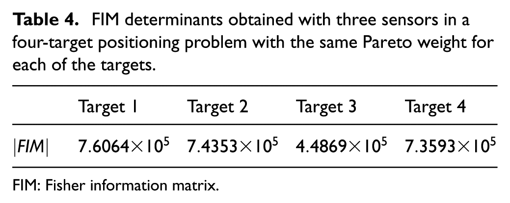
FIM determinants obtained with three sensors in a four-target positioning problem with the same Pareto weight for each of the targets.

	Target 1	Target 2	Target 3	Target 4
$|\mathrm{FIM}|$	$7.6064\times {10}^5$	$7.4353\times {10}^5$	$4.4869\times {10}^5$	$7.3593\times {10}^5$

FIM: Fisher information matrix.

Notice in Figure 4(a) and (b) how the maximum accuracy is over some of the targets, but how the accuracy is not the same for all the targets, and moreover, some of them have much larger accuracy than others while all the targets have the same Pareto weight. As mentioned above, this fact can be seen clearly in the FIM determinants listed in Table 4.

Figure 4.

Optimal formation for four-target positioning with the same Pareto weights: level curves of (a) $|\mathrm{FIM}{|}_{\mathcal{D}}$ in 2D and (b) $|\mathrm{FIM}{|}_{\mathcal{D}}$ in 3D.

In this last example, we can see clearly the problem of using only three sensors with more than two targets, and how in this situation the election of a trade-off solution, depending on the mission constraints and on the accuracy requirements for each of the targets, is imperative. If the feasible trade-off solutions with three sensors do not provide the required and desired accuracies, then we must adopt a solution with a larger number of sensors. This problem, that becomes non-convex, is analyzed in detail in the next section.

Extension to n sensors

In this section, we tackle the general problem of an arbitrary number of sensors and targets. It is important to remark that for more than three sensors, it is not possible to prove the concavity of the cost function in the search parameter space, and therefore, we must resort to non-convex optimization algorithms.

For the sake of simplicity, although the previous analysis for a three-sensor network was done with respect to the angles that the range vectors form between them, the optimization procedure used in this section will be carried out in the Cartesian coordinate space, that is, using the Cartesian coordinates of each of the sensors as design variables. The logarithm of the FIM determinant is not a concave function with respect to these variables, but with the knowledge that the maximum $|\mathrm{FIM}|$ is unique, and that this maximum is well defined for a single target, we have tools to determine whether the solution provided by the optimization process achieves desired conditions and whether it is close to the optimal value that would be obtained for a single target. For these reasons, a simulated annealing algorithm is used to determine the optimal sensor positions in this non-concave problem.

When several targets are working in collaborative and/or cooperative tasks, different levels of accuracy may be required for each of them. Notice from Examples 1 and 2 how the accuracy with which the estimates of the targets can be computed depends directly on the geometry of the sensor network. Moreover, in most of the practical problems, improving the accuracy in the estimate of one target may at times be done only in detriment of the accuracy of the other estimates, and thus, the trade-offs involved must be studied carefully. In this situation, the computation of the Pareto front showing these trade-offs between targets is of maximum interest to choose the “operation” points. Notice that in the problem at hand, the cost function is not concave and the solutions are computed with non-convex optimization tools, so strictly speaking it is not correct to name the representation of the trade-offs as Pareto front. For this reason, in what follows, it will be named as pseudo-Pareto front. The weights, for simplicity of explanation, will still be named as Pareto weights.

To obtain the optimal sensor configuration, as mentioned in previous sections, we maximize the cost function

$${\overline{p}}^{*}=\arg \underset{\overline{p}}{max}\sum _{k=1}^m{\lambda }_k\log \left|\mathrm{FI}{M}_k\right|$$

(14)

where $m$ is the number of targets involved in the multiple target positioning task, $\left|\mathrm{FI}{M}_k\right|$ is the FIM determinant for target $k$ , $\overline{p}$ is the vector of sensor positions, and ${\lambda }_k$ is the Pareto weight for target $k$ with $\sum _{k=1}^m{\lambda }_k=1$ . The weights ${\lambda }_k$ will be chosen depending on the mission constraints and/or the accuracy required for each of the targets.

The computation of the sensor positions is carried out using a simulated annealing algorithm. The philosophy of this algorithm is reproducing the behavior of the metal and ceramics annealing in which the material is heated and its cooling controlled, so the size of the crystals becomes larger and reduces their defects. In optimization, this meta-heuristic algorithm checks the neighbors of the present solution for a better solution (better state) to select. This process is repeated until a computational minimum is found or some conditions are met (maximum iterations, maximum time, a given threshold of accuracy, etc.). The advantage of this meta-heuristics algorithm resides in that it can avoid possible local minima and reach the global optimal, combined with small computation times.

The simulated annealing algorithm is run using the Global Optimization Toolbox of MATLAB. Once the solution is provided by the simulated annealing algorithm, a new optimization process is carried out with a constrained gradient optimization algorithm with the Armijo rule to refine the optimal solution. In the forthcoming example, it will be shown how the solution provided meets the desired specifications for the multiple target positioning problem.

Example 3

The target positioning problem studied in Example 2 is now revisited using a six-sensor network. The objective is to show the improvement in the accuracy with which the target positions can be estimated by using a larger number of sensors. Similar to the previous examples, the noise covariance is set to ${\sigma }^2=0.01{\mathrm{m}}^2$ for all the sensors, which are restricted to be placed in a squared region of $1000\mathrm{m}\times 1000\mathrm{m}$ with its center aligned vertically with the origin of the inertial coordinated frame $\{I\}$ . The Pareto weights have the same value for all the targets; it is ${\lambda }_k=0.25$ for $k=1,\dots ,4$ . The optimal sensor positions obtained after the optimization process are shown in Table 5 together with the target positions, which are the same positions defined in Example 2.

Table 5.

Optimal sensor positions and target positions for a four-target positioning problem with six sensors and the same Pareto weights for all the targets.

	x-coordinate (m)	y-coordinate (m)	z-coordinate (m)
Sensor 1	$91.2222$	$-0.9685$	$0$
Sensor 2	$37.4120$	$90.6019$	$0$
Sensor 3	$-37.4120$	$90.6019$	$0$
Sensor 4	$-91.2222$	$-0.9668$	$0$
Sensor 5	$-37.1143$	$-114.3485$	$0$
Sensor 6	$37.1143$	$-114.3485$	$0$
Target 1	$50$	$0$	$50$
Target 2	$-50$	$0$	$50$
Target 3	$0$	$75$	$50$
Target 4	$0$	$-100$	$50$

The FIM determinants obtained for each of the targets are shown in Table 6. Notice how the accuracy for all the targets is very similar, in contrast to that obtained in Example 2, and how the FIM determinants are close to the optimal one that would be obtained in a single target positioning problem, $|\mathrm{FIM}{|}_{\mathrm{opt}}=n^3/(3^3{\sigma }^2)=8\times {10}^6$ .

Table 6.

FIM determinants obtained with six sensors in a four-target positioning problem and the same Pareto weights for all the targets.

	Target 1	Target 2	Target 3	Target 4
$|\mathrm{FIM}|$	$6.8581\times {10}^6$	$6.8581\times {10}^6$	$6.9337\times {10}^6$	$6.4899\times {10}^6$

FIM: Fisher information matrix.

In Figure 5(a), we can see the optimal formation and the level curves of $|\mathrm{FIM}{|}_{\mathcal{D}}$ in region $\mathcal{D}$ . In Figure 5(b), these same level curves are shown in 3D to show clearly how the maximum values are over the target positions and how the accuracy degrades quickly when we move away from the target positions. This fact is very important for the practical problem in which the target positions are known with uncertainty and that will be studied in the “Uncertainty in the target positions” section.

Figure 5.

Optimal formation of six sensors for four-target positioning with the same Pareto weights for all the targets: level curves of (a) $|\mathrm{FIM}{|}_{\mathcal{D}}$ in 2D and (b) $|\mathrm{FIM}{|}_{\mathcal{D}}$ in 3D.

Therefore, comparing Example 3 with Example 2, if the number of sensors may be increased for a given number of targets, then the accuracy is improved significantly, making it possible to reach a similar accuracy for all the targets, and close to the optimal one that would be obtained for each of the targets working in isolation.

Examples for different Pareto weights

As mentioned in the “Multi-objective optimization and Pareto optimality” section, in multiple situations the physical or environmental constraints imposed by the mission, by the accuracies required for some of the targets, by the sensor network, and/or by the limited number of sensors that can be used force the election of a trade-off solution in which the accuracy of some targets is maximized while keeping the accuracy of the rest of the targets over a given threshold. Without loss of generality, the two examples studied next deal with two and three targets, respectively, because these are the two only possible scenarios in which it is feasible to compute a graphical representation of the pseudo-Pareto front. For more than three targets, the procedure would be exactly the same as the one described below. These examples are studied for different values of the Pareto weights, to make it clear how the sensor formation varies as a function of these weights in order to yield a Pareto-optimal solution.

Example 4

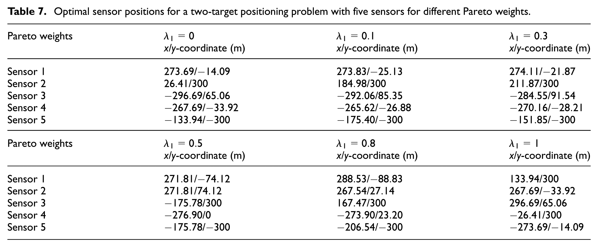
In this example, two targets are localized by a five-sensor network. In Example 1, it was shown that for two targets, it is possible to obtain for each target an accuracy similar to the one that would be obtained for a single target. This statement holds true if the sensors have enough freedom to be placed so that the optimal configuration may be reached. In the example at hand, the region where the sensors can be placed is bounded, and the targets are placed further from each other than in Example 1; thus, it is not possible to compute a sensor configuration that provides large accuracy for both targets simultaneously. The region where the sensors can be placed is a square area of $600\mathrm{m}\times 600\mathrm{m}$ with its center aligned vertically with the origin of the inertial coordinated frame $\{I\}$ , and the targets are over the $x_I$ axis, with 500 m between them and centered at the origin. In this particular case, a single Pareto weight ${\lambda }_1$ can be considered, since ${\lambda }_2=1-{\lambda }_1$ .

The optimal formation is computed for several values of the Pareto weight: ${\lambda }_1=0$ , ${\lambda }_1=0.1$ , ${\lambda }_1=0.3$ , ${\lambda }_1=0.5$ , ${\lambda }_1=0.8$ , and ${\lambda }_1=1$ . The corresponding optimal formations are listed in Table 7, and the values of the FIM determinants obtained for each of the targets and for each Pareto weight are shown in Table 8.

Table 7.

Optimal sensor positions for a two-target positioning problem with five sensors for different Pareto weights.

Pareto weights	${\lambda }_1=0$ x/y-coordinate (m)	${\lambda }_1=0.1$ x/y-coordinate (m)	${\lambda }_1=0.3$ x/y-coordinate (m)
Sensor 1	$273.69$ / $-14.09$	$273.83$ / $-25.13$	$274.11$ / $-21.87$
Sensor 2	$26.41$ / $300$	$184.98$ / $300$	$211.87$ / $300$
Sensor 3	$-296.69$ / $65.06$	$-292.06$ / $85.35$	$-284.55$ / $91.54$
Sensor 4	$-267.69$ / $-33.92$	$-265.62$ / $-26.88$	$-270.16$ / $-28.21$
Sensor 5	$-133.94$ / $-300$	$-175.40$ / $-300$	$-151.85$ / $-300$
Pareto weights	${\lambda }_1=0.5$ x/y-coordinate (m)	${\lambda }_1=0.8$ x/y-coordinate (m)	${\lambda }_1=1$ x/y-coordinate (m)
Sensor 1	$271.81$ / $-74.12$	$288.53$ / $-88.83$	$133.94$ / $300$
Sensor 2	$271.81$ / $74.12$	$267.54$ / $27.14$	$267.69$ / $-33.92$
Sensor 3	$-175.78$ / $300$	$167.47$ / $300$	$296.69$ / $65.06$
Sensor 4	$-276.90$ / $0$	$-273.90$ / $23.20$	$-26.41$ / $300$
Sensor 5	$-175.78$ / $-300$	$-206.54$ / $-300$	$-273.69$ / $-14.09$

Table 8.

FIM determinants obtained in a two-target positioning problem using five sensors for different Pareto weights.

Pareto weights	$|\mathrm{FIM}{|}_1$	$|\mathrm{FIM}{|}_2$
${\lambda }_1=0$	$2.9877\times {10}^6$	$4.6295\times {10}^6$
${\lambda }_1=0.1$	$3.4746\times {10}^6$	$4.6065\times {10}^6$
${\lambda }_1=0.3$	$3.5565\times {10}^6$	$4.5876\times {10}^6$
${\lambda }_1=0.5$	$4.1133\times {10}^6$	$4.1790\times {10}^6$
${\lambda }_1=0.8$	$4.5983\times {10}^6$	$3.5249\times {10}^6$
${\lambda }_1=1$	$4.6295\times {10}^6$	$2.9877\times {10}^6$

FIM: Fisher information matrix.

In Figure 6, the level curves of the FIM determinant over the region $\mathcal{D}$ for each optimal formation are shown together with the sensor positions. For the sake of simplicity, in contrast to previous examples, only the plots of the level curves of the FIM determinant in 2D are shown to avoid tedious repetition of similar plots.

Figure 6.

Optimal formations and level curves of $|\mathrm{FIM}{|}_{\mathcal{D}}$ in 2D for two-target positioning with five sensors for different Pareto weights: (a) ${\lambda }_1=0$ , (b) ${\lambda }_1=0.1$ , (c) ${\lambda }_1=0.3$ , (d) ${\lambda }_1=0.5$ , (e) ${\lambda }_1=0.8$ , and (f) ${\lambda }_1=1$ .

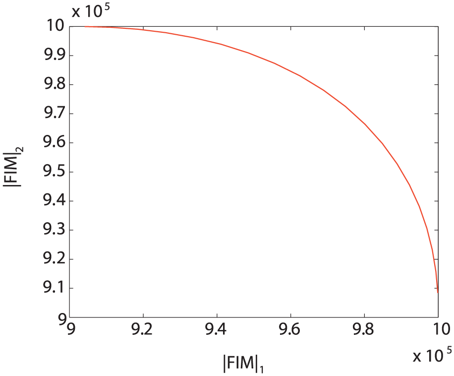
In Figure 7, the pseudo-Pareto front for the problem at hand is shown. Notice how the accuracies of the targets vary depending on the Pareto weight chosen.

Figure 7.

Pseudo-Pareto front for five sensors and two targets.

It is important to remark that in the extreme cases, ${\lambda }_1=0$ and ${\lambda }_1=1$ , the optimal formation has been searched as follows: by keeping the maximum theoretical accuracy possible in the corresponding target, $|\mathrm{FIM}|=4.6296\times {10}^6$ , maximize the accuracy of the remaining one. This has been done this way because it is possible to define several configurations that provide the optimal theoretical accuracy for a single target, and in a practical case, the chosen one would be the one between these possible solutions that provides the maximum accuracy possible for the remaining target.

Example 5

In this case, a five-sensor network is considered, which must be placed inside a square area of $600\mathrm{m}\times 600\mathrm{m}$ to localize three targets. The targets are placed at positions $q_1=[250,-100,-100]$ , $q_2=[-250,-100,-100]$ , and $q_3=[0,150,-100]$ . Several optimal configurations are studied for different values of the Pareto weights assigned to each of the targets. In Table 9, the optimal sensor positions obtained with the simulated annealing algorithm for the different cases of study are listed. In Table 10, the FIM determinants obtained in each of the different scenarios are also listed.

Table 9.

Optimal sensor positions for a three-target positioning problem with five sensors for different Pareto weights.

Pareto weights	${\lambda }_1={\lambda }_2=0.1$ , ${\lambda }_3=0.8$ x/y-coordinate (m)	${\lambda }_1={\lambda }_2=0.25$ , ${\lambda }_3=0.5$ x/y-coordinate (m)	${\lambda }_1={\lambda }_2={\lambda }_3=0.33$ x/y-coordinate (m)	${\lambda }_1={\lambda }_2=0.45$ , ${\lambda }_3=0.1$ x/y-coordinate (m)
Sensor 1	$58.68$ / $193.10$	$61.33$ / $174.32$	$2.62$ / $189.07$	$276.90$ / $-76.16$
Sensor 2	$-54.94$ / $172.21$	$-63.13$ / $199.07$	$-282.06$ / $-48.58$	$0$ / $206.84$
Sensor 3	$65.16$ / $-300$	$-288.37$ / $-96.56$	$-264.47$ / $-207.55$	$-276.90$ / $-76.16$
Sensor 4	$-289.92$ / $-99.20$	$-85.32$ / $-300$	$238.04$ / $-300$	$-253.08$ / $-300$
Sensor 5	$297.74$ / $-88.02$	$280.32$ / $-109.21$	$280.57$ / $-72.52$	$253.08$ / $-300$

Table 10.

FIM determinants obtained in a three-target positioning problem with five sensors for different Pareto weights.

Pareto weights	$|\mathrm{FIM}{|}_1$	$|\mathrm{FIM}{|}_2$	$|\mathrm{FIM}{|}_3$
${\lambda }_1=0.1$ , ${\lambda }_2=0.1$ , ${\lambda }_3=0.8$	$3.2817\times {10}^6$	$3.2174\times {10}^6$	$4.5736\times {10}^6$
${\lambda }_1=0.25$ , ${\lambda }_2=0.25$ , ${\lambda }_3=0.5$	$3.5708\times {10}^6$	$3.7289\times {10}^6$	$4.5222\times {10}^6$
${\lambda }_1=0.33$ , ${\lambda }_2=0.33$ , ${\lambda }_3=0.33$	$3.8866\times {10}^6$	$4.1313\times {10}^6$	$3.9591\times {10}^6$
${\lambda }_1=0.45$ , ${\lambda }_2=0.45$ , ${\lambda }_3=0.1$	$4.0728\times {10}^6$	$4.0728\times {10}^6$	$3.6798\times {10}^6$

In Figure 8, similar to Example 4, the plots of the level curves of $|\mathrm{FIM}{|}_{\mathcal{D}}$ in 2D are shown. Notice how depending on the weights assigned to the targets, their accuracies vary accordingly. This fact can be seen also in Table 10.

Figure 8.

Optimal formations and level curves of $|\mathrm{FIM}{|}_{\mathcal{D}}$ in 2D for three-target positioning with five sensors for different Pareto weights: (a) ${\lambda }_1=0.1$ , ${\lambda }_2=0.1$ , ${\lambda }_3=0.8$ ; (b) ${\lambda }_1=0.25$ , ${\lambda }_2=0.25$ , ${\lambda }_3=0.5$ ; (c) ${\lambda }_1=0.33$ , ${\lambda }_2=0.33$ , ${\lambda }_3=0.33$ ; and (d) ${\lambda }_1=0.45$ , ${\lambda }_2=0.45$ , ${\lambda }_3=0.1$ .

In Figure 9, the pseudo-Pareto front is shown. In this case, as we deal with three targets, this pseudo-Pareto front takes the form of a surface that defines the different trade-off solutions depending on the values of the Pareto weights.

Figure 9.

Pseudo-Pareto front for five sensors and three targets.

Therefore, we can see how it is possible to design optimal sensor configurations depending on the number of sensors, the number of targets, the weights assigned to each of the targets, and the constraints imposed to the sensor network. Of course, the methodology described can be applied to a larger number of targets, but for more than three targets, it is not possible to provide a graphical representation of the pseudo-Pareto front. However, the algorithms and problem formulation would be exactly the same, regardless of the number of targets and sensors; even the same procedure could be applied to define optimal formations in unconstrained 3D space, that is, without constraining the sensors to be placed in the same plane.

Uncertainty in the target positions

So far, the problem of optimal sensor placement has been studied with the assumption that the target and sensor positions are known without uncertainty. This assumption is unrealistic, and in a practical situation, the target positions are only known with uncertainty, that is, the only knowledge about the targets is that each of them is placed in a well-known region and its position inside this region is defined by a probability density function. In fact, even the sensor positions are not known with an exact precision, their positions are also known with uncertainty. The sensors are probably localized by GPS systems, so their positioning errors are generally small, depending on the quality of the systems used. Moreover, in multiple situations, the difficulty of keeping a vehicle in a static and precise position over the sea surface may make this uncertainty negligible. However, for the sake of completeness, in this section we formulate the optimal sensor placement problem considering that the target positions are defined by a probabilistic density function, and even that the sensor positions may be described by a probabilistic density function.

Let $\phi (p_i);p_i\in {\Re }^3$ denote the probability density function that describes the uncertainty of the sensor located at position $p_i$ and $\overline{p}=[p_1^T,\dots ,p_n^T{]}^T$ . Furthermore, let $\phi (q_k);q_k\in {\Re }^3$ be also a probability density function that describes the uncertainty of the $k\mathrm{th}$ target position in region $D\in {\Re }^3$ . With this notation, the optimal sensor placement problem can be cast in the form of finding a vector ${\overline{p}}^{*}$ such that

$${\overline{p}}^{*}=\arg \underset{\overline{p}}{max}\underset{D}{\int }\left|\mathrm{FIM}(\phi \left(\overline{p}\right),\phi \left(q_k\right))\right|\mathrm{dq}$$

(15)

where $|\mathrm{FIM}(\phi (\overline{p}),\phi (q_k))|$ represents the dependence of the FIM on the target and sensor locations and on their corresponding probability density functions. Following the notation adopted along the article, this later determinant will simply be denoted as $\left|{\mathrm{FIM}}_k\right|$ . In a real situation, on one hand, $\phi (p_i)$ will depend on the positioning device used to know the sensor positions. We consider that the sensors are carried by surface vehicles, so their positions are known by GPS, whose positioning errors are well known. On the other hand, $\phi (q_k)$ will depend on the a priori knowledge on the target positions and on the type of mission carried out by them. Then, the selection of the distribution functions will be clearly mission-dependent.

To define the optimal formation, the computation is carried out combining the simulated annealing algorithm with a gradient optimization using a MonteCarlo method. Therefore, in the initial step, the simulated annealing algorithm searches the sensor positions $\overline{p}$ that maximize equation (15) for well-known target positions that belong to the regions of interest, similar to the procedure described in the “Extension to n sensors” section. This solution is used in a second step as initial guess for the MonteCarlo gradient algorithm in which we include the probabilistic density functions of targets and sensors. In this case, the optimal formation depends largely on the probabilistic distributions that define the target positions, as it will be shown in the forthcoming examples. For this reason, in the following examples, the computation of optimal solutions will be done considering only the uncertainty in the target positions.

The two examples studied next deal with the problem of localizing two and three targets. Similar to the previous section, the optimal sensor formations are computed for different Pareto weights.

Example 6

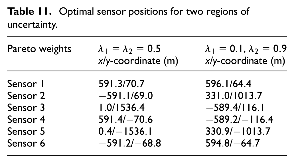
In this case, we consider that two groups of targets are working inside two different volumes of interest. In this particular example, the number of targets involved in the positioning task is of no relevance since they can only be working inside the areas of interest, and therefore, the sensor network must improve the average accuracy inside these volumes. Then, the probability density functions that define the uncertainty in these volumes are unity step distributions, which take the value of 1 inside the regions of interest and 0 outside them. For the areas of interest, we consider two volumes of $100\mathrm{m}\times 100\mathrm{m}\times 60\mathrm{m}$ with their centers aligned horizontally with the origin of the inertial coordinate frame {I} and separated by 500 m. A six-sensor network placed at 200 m over the origin of the inertial coordinated frame is used in this scenario. For the MonteCarlo method, 100,000 points per area of interest have been computed.

Two different situations are studied: first, when both areas are of the same importance, it is, the same Pareto weight, ${\lambda }_1={\lambda }_2=0.5$ ; and second, when one of the areas is far more important than the other, in the example studied, ${\lambda }_1=0.1$ and ${\lambda }_2=0.9$ . The optimal sensor configurations for these two cases are listed in Table 11.

Table 11.

Optimal sensor positions for two regions of uncertainty.

Pareto weights	${\lambda }_1={\lambda }_2=0.5$ x/y-coordinate (m)	${\lambda }_1=0.1$ , ${\lambda }_2=0.9$ x/y-coordinate (m)
Sensor 1	$591.3$ / $70.7$	$596.1$ / $64.4$
Sensor 2	$-591.1$ / $69.0$	$331.0$ / $1013.7$
Sensor 3	$1.0$ / $1536.4$	$-589.4$ / $116.1$
Sensor 4	$591.4$ / $-70.6$	$-589.2$ / $-116.4$
Sensor 5	$0.4$ / $-1536.1$	$330.9$ / $-1013.7$
Sensor 6	$-591.2$ / $-68.8$	$594.8$ / $-64.7$

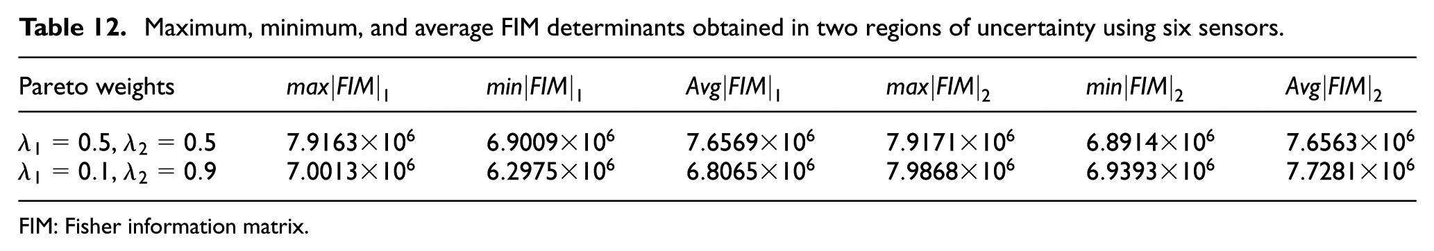
The maximum, minimum, and average values of the FIM determinants inside each of the work regions are shown in Table 12. Notice how for the first case, in which the Pareto weights are the same for both areas, the accuracies are very similar, the minimum FIM determinant obtained in these regions is very large and close to the maximum value, and therefore the average value in both areas is close to the optimal one. In the second case, where the Pareto weights are different, ${\lambda }_1=0.1$ and ${\lambda }_2=0.9$ , notice how the accuracy in the second region is larger than in the first one, consequence of the larger Pareto weight assigned to this region, providing an accuracy very close to the optimal one inside this volume. Moreover, it is interesting to notice how these different positioning accuracies between both cases of study are obtained with a slight change in the sensor configuration, allowing a fast adaptation of the sensor network to the mission requirements in a possible practical application. The optimal formations obtained can be seen in Figure 10(a) for ${\lambda }_1=0.5$ and ${\lambda }_2=0.5$ and in Figure 10(b) for ${\lambda }_1=0.1$ and ${\lambda }_2=0.9$ .

Table 12.

Maximum, minimum, and average FIM determinants obtained in two regions of uncertainty using six sensors.

Pareto weights	$\max |\mathrm{FIM}{|}_1$	$\min |\mathrm{FIM}{|}_1$	$\mathrm{Avg}|\mathrm{FIM}{|}_1$	$\max |\mathrm{FIM}{|}_2$	$\min |\mathrm{FIM}{|}_2$	$\mathrm{Avg}|\mathrm{FIM}{|}_2$
${\lambda }_1=0.5$ , ${\lambda }_2=0.5$	$7.9163\times {10}^6$	$6.9009\times {10}^6$	$7.6569\times {10}^6$	$7.9171\times {10}^6$	$6.8914\times {10}^6$	$7.6563\times {10}^6$
${\lambda }_1=0.1$ , ${\lambda }_2=0.9$	$7.0013\times {10}^6$	$6.2975\times {10}^6$	$6.8065\times {10}^6$	$7.9868\times {10}^6$	$6.9393\times {10}^6$	$7.7281\times {10}^6$

FIM: Fisher information matrix.

Figure 10.

Optimal sensor formations for different weights and two regions of uncertainty using six sensors: (a) ${\lambda }_1=0.5$ , ${\lambda }_2=0.5$ and (b) ${\lambda }_1=0.1$ , ${\lambda }_2=0.9$ .

Therefore, it is possible to obtain a large accuracy inside the working regions with an adequate sensor formation, whose configuration will directly depend on the number of regions of interest, the distribution functions that define the knowledge about the targets in these regions, and the number of sensors available for the task.

Example 7

In this example, we study the problem of three-target positioning. The areas that define the target positions are spherical Gaussian distributions with 30 m of standard deviation, with the center of the spheres at points $q_1=[550,500,0]$ , $q_2=[-550,500,0]$ , and $q_3=[0,-250,0]$ m. For these targets, two optimal configurations for different selections of the Pareto weights are studied. Moreover, these Pareto weights may change during the mission, so that the formation could dynamically change from one to another.

In Table 13, the optimal sensor positions are listed for the two different scenarios. In the first one, the Pareto weights are ${\lambda }_1={\lambda }_2={\lambda }_3=0.333$ , while in the second one, they are ${\lambda }_1=0.4$ , ${\lambda }_2=0.5$ , and ${\lambda }_3=0.1$ . The two optimal formations are shown in Figure 11.

Table 13.

Optimal sensor positions for three regions of uncertainty.

Pareto weights	${\lambda }_1={\lambda }_2={\lambda }_3=0.333$ x/y-coordinate (m)	${\lambda }_1=0.4$ , ${\lambda }_2=0.5$ , ${\lambda }_3=0.1$ x/y-coordinate (m)
Sensor 1	$645.1$ / $424.1$	$544.7$ / $610.9$
Sensor 2	$531.0$ / $657.1$	$613.1$ / $444.3$
Sensor 3	$-645.0$ / $424.1$	$-607.7$ / $450.9$
Sensor 4	$-530.9$ / $657.0$	$-551.3$ / $602.9$
Sensor 5	$-95.14$ / $-313.4$	$-736.1$ / $-1000.7$
Sensor 6	$95.10$ / $-313.4$	$602.6$ / $-1001.0$

Figure 11.

Optimal sensor formations for different weights and three regions of uncertainty using six sensors: (a) ${\lambda }_1={\lambda }_2={\lambda }_3=0.333$ and (b) ${\lambda }_1=0.4$ , ${\lambda }_2=0.5$ , ${\lambda }_3=0.1$ .

In the first scenario, in which the targets must be localized with similar accuracy, the sensors keep a regular formation, with a pair of sensors close to each of the regions of interest to provide the maximum global accuracy possible for all regions (see Table 14 and Figure 11(a)). Notice also how the accuracy of the third region is slightly larger than the other two, consequence of the target configuration and the number of sensors used. However, for the three regions, the accuracy obtained is large and close to the optimal one. In the second scenario, the Pareto weights have been selected to obtain a larger accuracy for regions 1 and 2 than for region 3. We can see in Table 13 and in Figure 11(b) how the sensors are now in a different configuration to provide the adequate accuracy for each of the regions. Notice in Table 14 how the accuracy for targets 1 and 2 is larger than for target 3, and also how the accuracy for target 2 is larger than for target 1, as expected according to the Pareto weights assigned.

Table 14.

Maximum, minimum, and average FIM determinants obtained in three regions of uncertainty using six sensors.

Pareto weights		$\max |\mathrm{FIM}|$	$\min |\mathrm{FIM}|$	$\mathrm{Avg}|\mathrm{FIM}|$
${\lambda }_1={\lambda }_2={\lambda }_3=0.333$	Region 1	$6.6288\times {10}^6$	$4.9777\times {10}^6$	$6.5178\times {10}^6$
	Region 2	$6.6286\times {10}^6$	$4.0621\times {10}^6$	$6.5176\times {10}^6$
	Region 3	$7.5750\times {10}^6$	$3.4439\times {10}^6$	$7.4118\times {10}^6$
${\lambda }_1=0.4$ , ${\lambda }_2=0.5$ , ${\lambda }_3=0.1$	Region 1	$7.5132\times {10}^6$	$3.8288\times {10}^6$	$7.4261\times {10}^6$
	Region 2	$7.6554\times {10}^6$	$4.5878\times {10}^6$	$7.5683\times {10}^6$
	Region 3	$7.6555\times {10}^6$	$0.3220\times {10}^6$	$1.6340\times {10}^6$

FIM: Fisher information matrix.

From this last example, we can notice how the methodology developed can be applied to multiple targets with different probability density distribution functions and different degrees of accuracy in a simple and fast manner, and therefore, that the methodology proposed may be applied to multiple scenarios and applications in marine robotics.

It is important to remark that we have considered a surface sensor network as an application case for the previous examples, but some of the sensors may be underwater and the procedure to define the optimal configuration would be exactly the same. For example, we may think on a sensor network in which some of the sensors are at the surface and another subgroup fixed at the sea bottom at known positions. In this case, we can design a sensor network by optimizing the surface sensors, or the whole network if we can modify the position of the sensors at the sea bottom. This alternative is not shown in this work for the sake of simplicity in the exposition of the algorithms and ideas on optimal sensor placement, but an example of this kind of sensor networks can be seen in Moreno-Salinas et al. ¹⁹ for single target positioning, where it is shown how it is possible to design the optimal sensor network with two groups of sensors, one at the sea bottom and the other at the sea surface.

Conclusion

In this article, we studied the problem of optimal sensor placement for multiple target positioning with only-range measurements. The application scenario in which a surface sensor network must localize a group of underwater targets was studied in depth. In a first step, the simplest problem of a three-sensor network was studied. In this particular scenario, it was demonstrated the concavity of the cost function used to compute the optimal sensor positions and how the optimal configuration can be computed using convex optimization tools. It was also shown that when more than two targets are involved in the positioning task, a three-sensor network may be insufficient to obtain a large accuracy for all the targets; thus, a trade-off solution must be adopted and Pareto optimization may be used to select the adequate configuration of the formation. In a second step, the problem was extended for a generic network of $n$ sensors to localize also an arbitrary group of $m$ targets. In this case, it is not possible to prove the concavity of the cost function, so non-convex optimization tools were used. A simulated annealing optimization algorithm was used to define several optimal sensor configurations depending on the mission constraints and the Pareto weights assigned to each of the targets. Finally, the above results were extended to the more realistic scenario in which the target positions are known with uncertainty, showing how the optimal formations depend on the probability density distribution functions that describe the knowledge about the target positions. Multiple simulation examples showed the effectiveness of the methodology and algorithms proposed and how the optimal sensor formation can be defined in an easy manner, regardless of the number of sensors or targets involved in the mission.