
Abstract
Although duty-cycling is a promising approach to reduce energy consumption in wireless sensor networks, sufficiently long network lifetime may not be achieved due to the hot spot problem. Moreover, a long duty cycle interval can lead to high end-to-end delay, which is not desired in delay-constrained applications. In order to address the hot spot problem and long end-to-end delay, this article proposes a novel energy-balanced node deployment algorithm for maximizing network lifetime in duty-cycled wireless sensor networks while taking into account a delay requirement. In addition, energy-balanced node deployment considers network connectivity and sensing coverage constraints, which are also important factors when wireless sensor networks are deployed. An optimization problem is first formulated where the objective function and constraints are estimated based on node distribution in the area and the network parameters. Then, a non-deterministic algorithm is proposed to derive the optimal number of nodes in each circular layer that meets given constraints and maximizes network lifetime. Numerical analysis and simulations have been conducted to validate the proposed algorithm. The results show that the proposed algorithm can achieve higher network lifetime than other schemes.
Introduction
A wireless sensor network (WSN) consists of a number of nodes deployed in the monitored area to collect and transmit data to a sink node. Due to the development of low-cost and multi-functional sensors, WSNs have been applied to many areas, including military, surveillance missions, and agriculture, among others.1–4 In WSNs, reducing energy consumption (i.e. prolonging network lifetime) has been attracting a lot of attention since sensors are usually provided with limited power. In this article, network lifetime is considered as the period from the time of WSN launch until the first node runs out of energy. 5 In order to prolong network lifetime, a duty-cycling technique can be used, in which nodes become active during a wake-up period, and sleep for the rest of a duty cycle interval. Although the duty-cycling method reduces energy consumption significantly, a long duty cycle interval can cause high packet delay, which is not desired in delay-constrained applications.1,2 Therefore, in WSNs for such applications, when duty cycling is used to lengthen network lifetime, a delay constraint should be considered, that is, packets are required to arrive at the sink within a certain time.
Moreover, network lifetime is highly affected by the hot spot phenomenon where some nodes need to transmit more packets than other nodes. 6 Specifically, nodes closer to the sink usually forward more data and they consume more energy than others. Hence, this hot spot issue reduces network lifetime considerably and causes unbalanced energy consumption in the network, that is, some nodes still have a lot of energy when the first node dies.
In order to deal with the hot spot problem, several node deployment algorithms were studied. Node deployment strategies can be classified into two types: deterministic and non-deterministic algorithms.
The former assumed that nodes have the same capabilities, such as transmission range and initial energy budget.7–12 Then, in order to balance energy consumption, they determine the number of nodes and positions of the nodes, and place nodes in pre-determined positions. Although deterministic deployment algorithms can control sensing coverage and network connectivity, this approach requires the exact positions of the nodes, which is costly and impractical.
To avoid pre-determined deployment, the latter (non-deterministic node deployments) can be used, in which nodes do not need to be placed at pre-determined positions. According to node distribution, we may classify non-deterministic node deployment schemes into two groups: uniform and non-uniform node distributions.
In the first group, nodes are deployed randomly with a uniform distribution throughout the whole area.12–19 Note that since the positions of the nodes are random variables, it is important to satisfy sensing coverage and network connectivity constraints with the desired probability. However, none of those works12–19 considered network connectivity, sensing coverage constraints, and a delay requirement. In the second group, the authors estimated node distribution in each region according to data traffic in the area in order to prolong network lifetime.20–22 Node density in the regions can be different from each other. However, neither of those studies20–22 considered the delay bound that is required in delay-constrained applications. For example, although Liu et al. 22 considered network connectivity and sensing coverage constraints, they did not address the delay requirement. In addition, some node deployment algorithms required a large number of nodes to maximize network lifetime.13,20
In order to address the limitations in existing algorithms, we propose a novel non-deterministic energy-balanced node deployment algorithm (EBND), which determines the appropriate number of nodes in each circular layer in order to maximize network lifetime while satisfying delay, network connectivity, and sensing coverage constraints in duty-cycled WSNs. Unlike several schemes that required a large number of nodes, EBND can determine the number of nodes in each region given total number of nodes. This brings great flexibility to our algorithm compared to existing ones.
In this article, we first formulate an optimization problem to maximize network lifetime with constraints on packets delay, network connectivity, and sensing coverage, which are estimated as a function of the number of nodes in each circular layer. Then, an algorithm is proposed to find the optimal number of nodes in each layer in order to maximize network lifetime while satisfying the constraints. Numerical analysis and extensive simulations have been conducted to validate the proposed algorithm by comparing with other node deployment schemes under different network parameters. Numerical results indicate that EBND requires a smaller number of nodes and consumes less energy than Olariu’s algorithm. 13 Moreover, simulation results show that EBND can achieve longer network lifetime than other deployment schemes while satisfying the required constraints.
The rest of this article is organized as follows. The sections “Related work” and “System model and assumption” describe existing work and the system model, respectively. Then, the “EBND with delay, network connectivity, and sensing coverage requirements” section presents the main algorithm in detail. Numerical results and the performance study are presented in the sections “Numerical results” and “Performance study,” respectively. Finally, the section “Conclusion” concludes the article and discusses future work.
Related work
In this section, we describe several existing node deployment algorithms and then compare these schemes with ours. Node deployment schemes can be classified into deterministic7–12 and non-deterministic.12–22
In deterministic node deployment, the number of nodes in each region and all nodes’ positions are estimated in order to satisfy a given requirement, such as maximizing network lifespan or balancing energy consumption. The strength of this kind of deployment is network connectivity and sensing coverage can be controlled strictly. However, it is clear that the cost of this deployment is high, especially when the total number of nodes and total area size increase.
For instance, two well-known deterministic node deployments were presented: grid and tri-hexagon tiling (THT) schemes. 12 In the grid deployment method, the entire area is divided into a grid of cells where each crosspoint hosts a sensor node. In the THT scheme, the authors considered semi-regular tiling that uses triangles and hexagons in a two-dimensional plane. Nodes are placed at the vertices of the triangles or hexagons. Although the authors evaluated and compared energy consumption, k-coverage, and packets delay between these schemes, they did not consider the constraints of delay, network connectivity, and sensing coverage.
Wu et al.
9
considered sensor nodes that are deployed in a circular area with multiple layers, and all sensors were homogeneous and used the same maximum transmission range. The authors defined sub-balanced energy consumption as a feature where nodes in all layers (except the outermost) run out of energy simultaneously. In order to achieve sub-balanced energy depletion, the number of nodes in each layer should be greater than that in the farther layer by
In order to achieve better balanced energy consumption and longer network lifetime than Wu’s scheme, Ferng et al. 7 proposed three node distribution strategies. Sensor nodes that have the same transmission range are deployed in an area with multiple concentric layers. Since there is a large number of redundant nodes in inner layers, it is not necessary for nodes to turn on and to sense the environment all the time. The authors calculated the minimum number of nodes in each layer in order to fully cover the monitored area, and only those nodes are allowed to sense and transmit data to the sink at any one time, while other nodes in the layer are in sleep mode. That reduced the number of generated packets. Therefore, energy consumption for transmitting and receiving data is much reduced, and network lifetime can be prolonged.
However, both of Wu’s and Ferng’s schemes use deterministic node deployment algorithms, that is, nodes are required to be placed at exact, pre-determined positions. This is impractical, especially in a large area. Therefore, in this work, we propose a non-deterministic node deployment algorithm that does not require placing nodes at pre-determined locations. Moreover, the proposed algorithm takes into account delay, sensing coverage, and network connectivity constraints, while the above-mentioned algorithms do not.
Unlike deterministic node deployment strategies, non-deterministic deployment algorithms13–21 do not require pre-determined placement of nodes, and most of them tried to address the problem of network lifetime maximization by adjusting the transmission range or determining node density in each area. For example, uniform random deployment 12 was presented, in which nodes are deployed randomly with a uniform distribution throughout the whole area. Although the authors compared energy consumption, coverage, and packets delay against grid and THT node deployments, they did not try to maximize network lifetime or satisfy sensing coverage, network connectivity, and delay constraints.
Olariu and Stojmenovi 13 studied the problem of balancing energy consumption, or maximizing network lifetime in the network, by finding the appropriate transmission range for nodes in each layer. The entire area is divided into multiple concentric layers where nodes are scattered randomly with a uniform distribution. The authors formulated energy consumption of nodes in each layer as a function of the transmission range of nodes in layers along with other parameters. In order to balance energy consumption, they derived a set of transmission ranges of nodes in layers, which increases from the innermost to the outermost layer as predicted. However, since the obtained transmission range is much lower than the maximum transmission range, Olariu’s scheme requires many more nodes than other algorithms that use the maximum radio range.
Song et al. 14 aimed at maximizing network lifetime by adjusting transmission ranges of nodes for each layer in the WSN. They assumed that nodes in the same layer have the same transmission range and, for a given node deployment, network lifetime of the nodes is calculated as a function of node transmission ranges and other network parameters, 14 such as the number of nodes in each layer and the layer’s width. Therefore, among a list of possible transmission ranges, they can obtain a set of transmission ranges that achieves maximal network lifetime. Since searching for an optimal set of transmission ranges is non-deterministic polynomial-time (NP)-hard, they proposed two heuristic algorithms to obtain a nearly optimal list with lower complexity. However, requirements of delay, sensing coverage, and network connectivity were not considered in their work.
Demertzis and Oikonomou 20 proposed a non-uniform node distribution in order to address energy hole problem and to prolong network lifetime. The authors used two kinds of sensor node: active and dormant. While active nodes sense and transmit data, dormant nodes work as energy reservoirs, that is, when an active node exhausts its energy, a nearby dormant node becomes active. According to traffic load, the density of dormant nodes is determined in each region. Then, active nodes are deployed randomly with a uniform distribution through the whole area, while dormant nodes are scattered with a higher node density for closer regions to the sink. However, this algorithm requires a large number of nodes, for example, the number of dormant nodes is roughly 10 times higher than active nodes. Compared to EBND, some of the non-deterministic algorithms required a large number of nodes.13,20
There were several studies on maximizing network lifetime under different quality of services (QoS) constraints. However, QoS constraints in EBND differ from existing work.23–25 Specifically, in Xiao et al.,
23
each node is randomly assigned into one of
The concentric layers infrastructure was discussed in existing studies of maximizing network lifetime in WSNs13–15 in which a number of sensors are deployed in an area with the sink at the center of that region. Sensors are classified into concentric layers according to their distances to the sink. Note that although the concentric rings feature is used in this work, EBND considers WSNs with non-uniform node deployment while uniform node distribution was assumed in literatures.13–15 Moreover, given the assumption that nodes are provided with the same transmission range, EBND determines the number of nodes in each layer in order to maximize network lifetime under desired constraints. Whereas, Olariu and Stojmenovic, 13 Song et al., 14 and Tran-Quang and Miyoshi 15 considered nodes with the adjustable communication range in order to lengthen network lifetime in WSNs.
System model and assumption
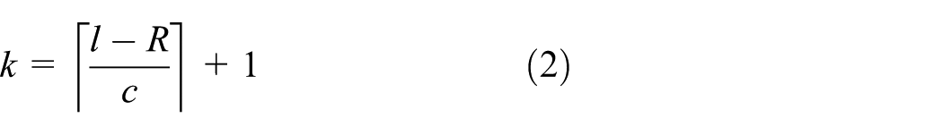
In this work, we assume that nodes are deployed in a circular area with the sink node at the center, and each node knows its position. Nodes are assumed to have the same transmission range,

where
Let

Define

Let random variable

Network model.
Sensors use a duty-cycling strategy, that is, nodes turn on the radio during an active period and turn it off for the rest of duty cycle interval
Let potential forwarders of a node represent all neighboring nodes belonging to the forwarding area. When it has a data packet, the sender waits until a node among all potential forwarders wakes up and forwards the packet to the node that wakes up earliest. Since a node is able to predict the schedules of its neighbors, the sender should be in sleep mode until the next hop becomes active. This strategy can help nodes reduce energy consumption by turning off the radio when unnecessary.
In this article, the energy model is the one referred in Heinzelman et al.
28
On the transmitter side, there are transmission electronics and a transmission amplifier, while the receiver side consists of reception electronics. Transmission power
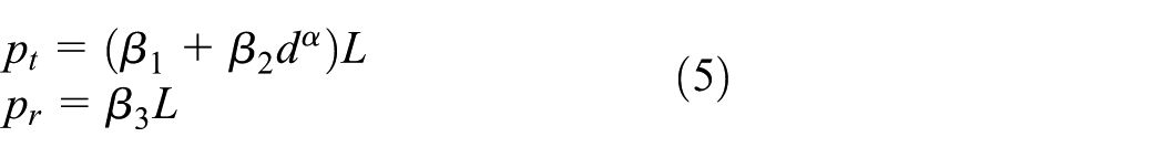
where
EBND with delay, network connectivity, and sensing coverage requirements
In this section, we study an optimization problem with the objective of maximizing network lifetime while satisfying the delay, network connectivity, and sensing coverage requirements given the number of nodes. First, the problem definition is presented. Then, we describe the objective function and constraints as a function of the number of nodes in layers. Finally, the full problem formulation and the proposed algorithm are discussed.
Problem definition
We define the critical node as the node that consumes energy the most in the network. It is not known a priori which node in the network will be the critical node. The layer to which the critical node belongs is called the critical layer.
Then, the problem is to minimize the energy consumption of the critical node (i.e. maximize network lifetime) while satisfying the required delay, network connectivity, and sensing coverage given the total number of nodes.
Let
Also, let
Then, the optimization problem can be defined as follows

subject to


The objective function implies that we maximize network lifetime by minimizing the energy consumption of the critical node. Recall that it is not known which node among
Equation (7) shows the expected delay of all nodes in the network should be less than the delay constraint. In addition, constraints of network connectivity and sensing coverage are presented in equations (8) and (9), respectively. In the next subsections, the objective function and constraints are discussed in detail.
Energy consumption
We first present the total energy consumption of nodes in layer

where
Note that since nodes in the same layer are deployed randomly using the uniform distribution and they randomly choose the wake-up time during the node interval, nodes in the same layer can be considered to have the same probability of being selected as the next forwarder. Therefore, by the law of large numbers, 29 the remaining energy of nodes in a layer will have the same value when the network operation time is sufficiently long.
Therefore, in order to minimize the energy consumption of the critical node, we minimize the energy consumption of an arbitrary node in the critical layer, and the objective function can be rewritten to address the problem of minimizing the energy consumption of an arbitrary node in the critical layer.
Let

Then, by the definition of the critical layer, the objective function is equivalent to minimizing

Delay constraint
Note that the expected delay of packets from nodes in the outermost layer is longer than the delay from the inner layers. If nodes in layer
Expected latency
We consider a node in layer

Now, distribution function

where

Then, the expected one-hop latency of nodes in layer

where
After applying a Taylor expansion for function

Define
Define

where the
Network connectivity and sensing coverage
In WSNs, network connectivity and sensing coverage should be guaranteed with a desired probability. In this subsection, we estimate the minimum number of nodes, or, the minimum node density, that satisfies both network connectivity and sensing coverage constraints. Node density,
First of all, we take into account the required network connectivity that is presented in equation (8). Recall that

Note that if nodes in the outermost layer satisfy the required network connectivity, nodes in other layers also satisfy this constraint. Hence, the sufficient condition to achieve the network connectivity requirement can be written as follows

From equation (20), since

Let

The necessary condition is used to narrow the range of number of nodes in each layer. Note that nodes in the outermost layer do not relay data packets, so there is no required node density for the outermost layer, that is,
Second, we consider the required sensing coverage that is described in equation (9). Recall that

Recall that

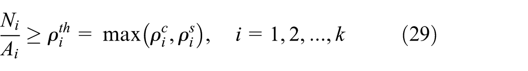
Finally, we determine the node density threshold in circular layer

Recall that

Problem formulation
Finally, using equations (12), (18), (25), and (26), the problem can be formulated as follows

subject to


Equation (27) implies that the energy consumption of the critical node is minimized. Recall that the energy consumption of an arbitrary node in layer

where
Algorithm
In order to solve the optimization problem, all feasible cases are examined. The algorithm works as follows:
Set the optimal number of nodes in each circular layer,
For each feasible set of
Among the sets of
The formal algorithm is presented in Algorithm 1. In order to determine the time complexity of the proposed algorithm, first, we obtain the number of feasible cases to deploy

Numerical results
In this section, we compare EBND with Olariu’s scheme. 13 MATLAB was used to validate these algorithms. The required number of nodes and the total energy consumption of all nodes in the network are selected as performance metrics. We first briefly summarize Olariu’s scheme. Then, we present the network parameters and how to calculate energy consumption. Finally, the obtained results with different network parameters are analyzed.
In Olariu’s scheme, the transmission range of a node in layer
The communication energy parameters (

where
The total energy consumption in the network can be estimated as follows

where
In this section, the transmission range and sensing range are set to 30 and 10 m, respectively. The area radius changes from 60 to 100 m. The network connectivity requirement,
The difference between EBND and Olariu’s scheme is that instead of using a random node deployment with a uniform distribution, EBND determines the appropriate number of nodes
As shown in Figure 2, with the greater area radius or the greater required network connectivity

Comparison with Olariu’s scheme: (a) the total number of nodes and (b) the total energy consumption.
This result is attributed to the following fact. In Olariu’s scheme, the transmission range of nodes in inner layers is much smaller than the maximum radio range. For example, when the area radius is set to 80 m, the transmission ranges of nodes in layers 1 to 5 are {8.19, 16.02, 21.64, 28.82, 28.82} m, respectively. More specifically, nodes in layer 1 can only transmit a signal up to 8.19 m, while the maximum radio range is 30 m. The connectivity range of these nodes is reduced
Performance study
In this section, we present a performance comparison between EBND and three well-known node deployment strategies, 12 that is, random, grid, and THT node deployments. We do not take into account Olariu’s scheme 13 because Olariu’s method requires a large number of nodes and high consumed energy as discussed in the previous section.
Simulation setup is shown in Table 1. The bold numbers are the default values. In order to provide high network QoS, high values of network connectivity and sensing coverage requirements (i.e. 0.99 and 0.995, respectively) are chosen. Several parameters of the Mica mote family
30
are used, that is, the transmission range and transmission rate of nodes. Layer width
Network parameters.

Bold texts highlights the default values.
For routing protocols, LF and lukewarm potato forwarding (LPF) 31 are considered in order to evaluate network performance under different routing algorithms. Since LPF is a geometric routing algorithm that aims to achieve low packet delay in WSNs, we select LPF as a routing algorithm in addition to the proposed routing algorithm, LF.
Packet delivery ratio (PDR), average E2E delay, network lifetime, and average energy consumption are selected as performance metrics. Network parameters include the number of nodes, the area radius, and the sensing range. Network simulator 2 (NS2) is used to validate algorithms. Simulation results show that EBND outperforms random, grid, and THT node deployment schemes in terms of network lifetime, PDR, E2E packet delay, and average energy consumption.
The following subsections will discuss the obtained results in more detail.
Effects of number of nodes
We compare EBND with three other node deployment strategies that use two forwarding schemes, LF and LPF. The number of nodes varies from 300 to 450 while other parameters remain unchanged. According to the given number of nodes, EBND determines the optimal number of nodes in each layer. For example, given 375 sensor nodes, the number of nodes from the innermost layer to the outermost is {100, 74, 54, 47, 59, 41}, respectively.
As shown in Figure 3, with both routing algorithms, EBND achieves a higher PDR than random, grid, and THT node deployments. This is attributed to the fact that EBND alleviates the hot spot problem while other algorithms do not, that is, in EBND, the congestion caused by a many-to-one traffic pattern is reduced. In addition, EBND considers the required network connectivity that is 0.99 in the simulation setup. Therefore, PDR in EBND is higher than other evaluated node deployment methods. Moreover, Figure 3 shows that EBND results in smaller average E2E packet delay than three remaining node deployment schemes. The main reason is that EBND considers the required delay constraint while trying to balance energy consumption.

PDR and average E2E delay with different numbers of nodes: (a) LF scheme and (b) LPF scheme.
In addition, Figure 4 illustrates network lifetime of EBND is always higher than that of random, grid, and THT node deployment schemes under both LF and LPF forwarding schemes. This result is due to the following reasons. In EBND, we deploy nodes based on the traffic in each layer in order to reduce the unbalanced energy problem, that is, the greater traffic, the more nodes we assign to the area. Unlike EBND, random, grid, and THT do not consider the amount of traffic, which leads to the many-to-one traffic pattern, or the hot spot problem. As a result, nodes in inner layers consume much more energy than other nodes. Therefore, network lifetime under these schemes is shorter than it is under EBND.

Network lifetime with different numbers of nodes: (a) LF scheme and (b) LPF scheme.
Moreover, in EBND, when the number of nodes increases, we can place more nodes in the high traffic area to balance energy consumption. Hence, network lifetime can also be improved given the higher number of nodes. For example, when the number of nodes changes from 300 to 450, Figure 4(a) shows that network lifetime in EBND with the LF algorithm improves
In contrast, the number of nodes does not affect network lifetime much in the three other schemes, that is, random, grid, and THT. As shown in Figure 4, when the number of nodes increases, network lifetime of three counterparts remains similar. This is due to the following reason. When the higher number of nodes is provided, both the number of nodes in each layer and the number of data packets forwarded from further layers increase at the same ratio. Hence, the traffic load of a node in each layer is actually unchanged; in other words, network lifetime cannot be improved by requesting more nodes. For example, Figure 4(a) illustrates that network lifetime under the random node deployment is {1411.4, 1220.9, 1411.29, 1181.6, 1412.62, 1358.88, 1425.9} while varying the number of nodes from 300 to 450 under the random deployment.
Note that, even with the LPF scheme, EBND achieves the higher performance (including network lifetime, PDR, average E2E delay, and energy consumption) than three considered node deployment methods. The reason is as follows. EBND aims at reducing the hot spot problem that is unavoidable in a lot of routing algorithms, for example, LPF. Therefore, although LPF is used as a forwarding scheme, the energy consumption of EBND is more balanced and network lifetime can be prolonged compared with three considered methods. PDR performance can also be improved due to the fact that the congestion is reduced. The delay constraint in the EBND node deployment algorithm helps to reduce the average E2E delay even in case of LPF.
As also shown in Figure 4, EBND under the LF scheme shows higher network performance than EBND under LPF. For example, when the number of nodes is 375, network lifetimes of EBND are 5003.94 and 3765.2 s in cases of LF and LPF, respectively. The main reason is that, in LPF, nodes are likely to forward packets to a specific neighboring node, called node’s parent, rather than other neighbors, that is, this specific node tends to experience the high traffic issue. As a result, the energy consumption in the LPF routing algorithm is more unbalanced and network lifetime is lower than LF.
Effects of area radius
In this subsection, we compare EBND to random, grid, and THT deployments with different area radii, under two forwarding schemes, LF and LPF. The area radius is set to {225, 243.8, 262.5, 281.3} m. In EBND, the number of nodes in each layer is obtained using Algorithm 1, for example, when the area radius is 225 m and the number of layers is five, the obtained number of nodes from layer 1 to layer 5 is {155, 91, 53, 41, 35}, respectively.
Figure 5 shows that PDR performance in other node distribution algorithms drops sharply, but PDR in EBND does not. The result comes from the fact that EBND tries to alleviate the many-to-one traffic pattern that causes congestion and collision in WSNs. Therefore, EBND can achieve a higher PDR than three considered node deployment schemes. In terms of E2E delay, EBND results in the lowest packet delay among the considered node distribution strategies. The reason is attributed to the fact that, in EBND, data packets are forwarded to the sink within the desired delay constraint while other algorithms do not take the delay requirement into account.

PDR and average E2E delay with area radii: (a) LF scheme and (b) LPF scheme.
Moreover, as shown in Figure 6, under all node deployment strategies, network lifetime decreases with a greater area radius. This is attributed to the following fact. In EBND, first, the number of nodes satisfying sensing coverage and network connectivity is determined, and then, the remaining nodes (m) are assigned in such a way as to balance energy consumption. If the larger area is considered, the number of nodes required to meet sensing and network coverage constraints increases. Therefore, a smaller number of remaining nodes is assigned in the hot spot area to balance energy consumption. That causes decreased network lifetime under EBND. Meanwhile, in random, grid, and THT deployments, with the greater area radius and the fix number of nodes, node density decreases; that is, there are fewer nodes in the hot spot area, and these nodes need to forward more packets from further layers. This leads to decreased network lifetime. For example, with the THT node deployment and the LF routing scheme, network lifetime is {3300.64, 2502.75, 1606.74, 1169.42} s when the area radius is {225.0, 243.8, 265.0, 281.3} m, respectively.
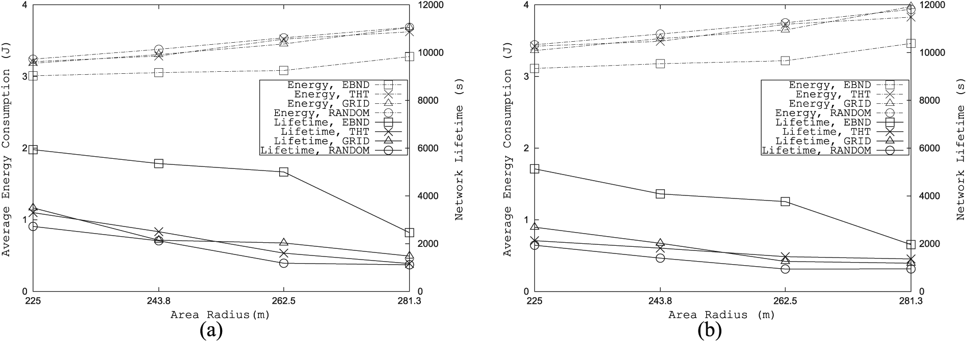
Network lifetime with area radii: (a) LF scheme and (b) LPF scheme.
Although network lifetime under the four node deployment strategies decreases, EBND always achieves the highest network lifetime compared to the three other algorithms. Unlike the three remaining algorithms, EBND deploys nodes based on the traffic in each layer in order to balance energy consumption as much as possible while satisfying delay, network connectivity, and sensing coverage constraints.
Figure 6 also shows that the increased average energy consumption is observed with a greater area radius. Specifically, there are more nodes in farther layers, that is, the average distance from the nodes to the sink is longer, and the average number of packet transmissions increases. Therefore, in four considered node deployment schemes, nodes spend more energy due to the increased area radius.
Effects of sensing range
In this subsection, we discuss the effect of sensing range on network performance in EBND, random, grid, and THT node deployments under LF and LPF routing algorithms. The sensing range is set to {37.5, 50, 75, 100} m while other parameters are kept constant. As can be seen from Figures 7 and 8, the sensing range only affects the network performance under EBND. In EBND, when the sensing range increases, the minimum number of nodes that meets the requirement of sensing coverage is smaller; that is, we can assign more nodes in crowded regions or inner layers to balance energy consumption, and hence, network lifetime increases. For instance, under the LF routing algorithm, when the sensing range varies from 37.5 to 100 m, network lifetime is enhanced 1.37 times, from 4082.68 to 5615.88 s, respectively.
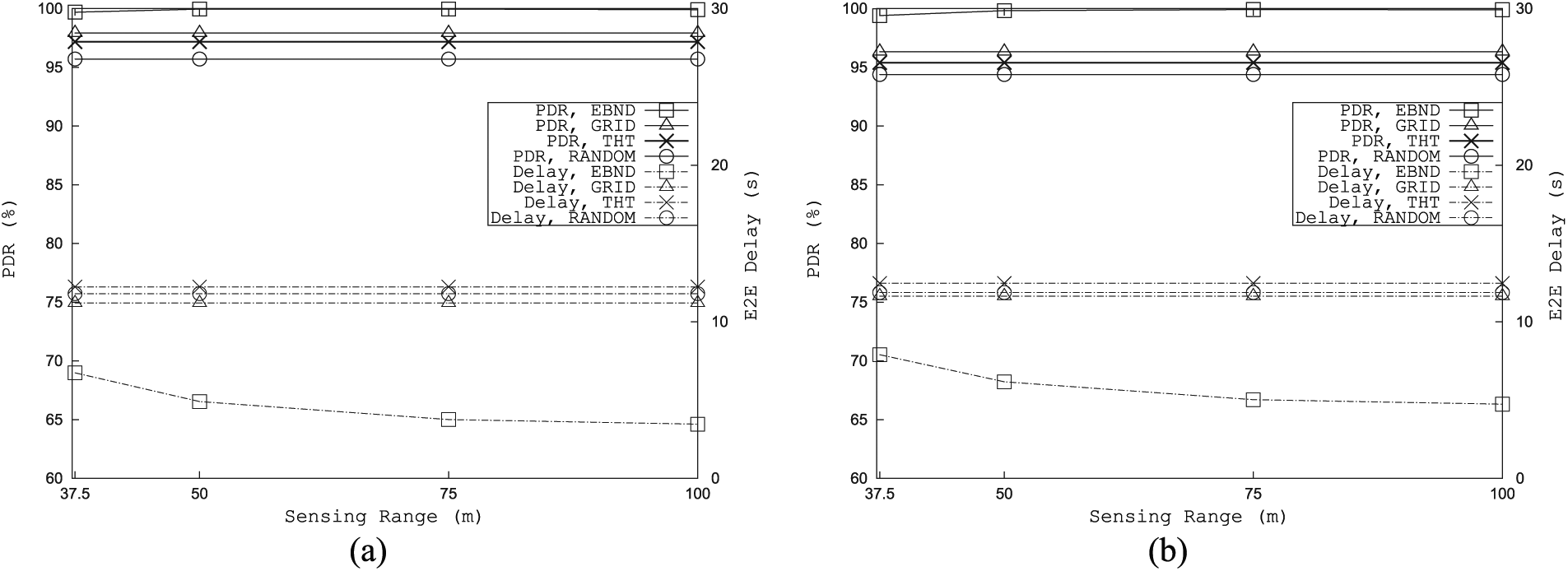
PDR and average E2E delay with sensing ranges: (a) LF scheme and (b) LPF scheme.

Network lifetime with sensing ranges: (a) LF scheme and (b) LPF scheme.
Meanwhile, under EBND, the average E2E delay and average energy consumption decrease with the greater sensing range. This is because there are more nodes deployed in inner layers, and these nodes in the inner layers have lower delay and energy consumption than nodes in outer layers. Therefore, the average E2E packet delay and energy consumption decrease.
Note that only EBND considers the sensing coverage constraint, whereas random, grid, and THT schemes do not. Hence, there is no change in network performance with the different sensing ranges under the random, grid, and THT schemes.
Conclusion
This article addressed the issue of maximizing network lifetime considering delay, sensing coverage, and network connectivity constraints in WSNs. A novel EBND algorithm called EBND was proposed, in which we formulate an optimization problem to determine the optimal number of nodes in each layer to maximize network lifetime with multiple constraints.
In EBND, the objective function and constraints are estimated as a function of the number of nodes in the layers. We proposed an algorithm to attain the optimal number of nodes in each layer, given the total number of nodes. Numerical results indicate that EBND demands a smaller number of nodes and less consumed energy than Olariu’s scheme. Simulation results show that EBND can achieve longer network lifetime than other node deployment strategies considered while satisfying the constraints.
Footnotes
Handling Editor: Ju Wang
Declaration of conflicting interests
The author(s) declared no potential conflicts of interest with respect to the research, authorship, and/or publication of this article.
Funding
The author(s) disclosed receipt of the following financial support for the research, authorship, and/or publication of this article: This work was supported by the 2016 Research Fund of University of Ulsan.