Sage Journals: Discover world-class research

Abstract

Wireless sensor networks (WSNs) have attracted intense interest due to their extensible capability. In this paper, we attempt to answer a fundamental but practical question: how should we deploy these nodes. In most current designs, sensor nodes are randomly or uniformly distributed because of their simplicity. However, the node deployment has a great impact on the performance of WSNs. Instead of maintaining the coverage for some snapshots of a WSN, it is essential that we can provide a continuous coverage in the whole lifecycle of the WSN. We will exhibit the weakness of the uniform distribution by disclosing the fatal sink routing-hole problem. To address this problem, we propose a non-uniform, power-aware distribution scheme. Our analysis and simulation results show that the power-aware deployment scheme can significantly improve the long-term network connectivity and service quality.

Keywords

Wireless Sensor Networks Node Deployment Sensing and Connectivity Coverage

1. Introduction

Recent advances in electronics and wireless communications gave rise to sensor applications ranging from environmental monitoring and pollution detection to feature extractions [1, 2]. Battery-powered sensor nodes are integrated with sensing, local processing, and communication capabilities [3]. They are characterized as tiny devices with constrained resources. Due to large—scale deployment, recharge or reuse of sensor nodes is costly and implausible. Therefore, the power issue arises as the key of the design objective. In particular, the transceiver, including the transmitter and receiver, contributes to the greatest energy consumption [4].

Among many challenging issues, in this paper we discuss a fundamental and practical problem, how we should deploy these sensor nodes, or what node-deployment function is an optimal for sensors. In most current designs, random and uniform distributions are the popular schemes due to their simplicity. However, as we will show later, node deployment related issues have a great impact on the system functionality and lifetime. The traditional random and uniform distributions are not suitable because of the sink routing-hole phenomenon. Instead, we propose a non-uniform, power-aware node deployment scheme which is the main focus in this work.

One may be concerned as to whether a desired node deployment function is practical to be carried out. In fact, the advances in robotics and automations have made it possible to realize an autonomous sensor deployment by unmanned aerial vehicles [5]. It enables the deployment of individual nodes and thus makes a well-designed distribution function feasible. However, this part of the work is beyond the scope of this paper. Interested readers may refer to [5] for more details.

Concerning the unique features, WSNs are inherently different from existing systems and networks. Unlike traditional mobile ad-hoc networks (MANETs), in WSNs one or a set of nodes (called sink) are designated as gateways between the networked system and users. These sinks account for the critical role of the network as their loss directly leads to the failure of the entire WSNs. Furthermore, not only the sink but the direct neighbors of the sink are also essential for network functionality. An example is shown in Fig. 1 . The shaded area represents the region containing the direct neighbors of the sink. They are required to establish and maintain the connectivity between the sink and distant data nodes. When this set of nodes fails, no data can be delivered to the sink due to the lack of forwarders and thus the whole system fails. Often the sinks are more powerful with permanent power sources. Their failure may not be frequent. However, their nearby neighbor nodes are common sensor nodes with limited resources. These nodes are vulnerable to failure (e.g., running out of energy). An interesting observation is that for most data gathering applications the forwarding workload of sensors increases inversely with their distances to the sink. A node closer to the sink usually has a higher relay workload than those of farther nodes. Accordingly, direct neighbors of the sink have the greatest transmitting workload. They are likely to deplete their energy at the very beginning. When they fail, no matter how many remaining nodes are still active, none of them can communicate with the sink. From the sink and user's perspective, the whole system fails if the sink is isolated from the rest of the sensor nodes. Such a scenario is referred to as the “sink routing-hole” phenomenon. Note that multiple sinks [6] or mobile sinks cannot eradicate the problem as many sink routing-holes will be generated accordingly. Data funneling and aggregation [7] techniques may alleviate the problem to some extent, but cannot eliminate the problem either.

Figure 1

An example of sensor network transmission paradigm.

The main objective of our work is to provide a long-term continuous connectivity. We attempt to address the problem by designing a power-aware deployment scheme. Major attention is paid to the connectivity of the network as it is a prerequisite for other purposes such as sensing coverage. Note that without a valid data path, an active node has the same role as a dead one. The sensing area covered by unconnected nodes is still inaccessible. However, traditional approaches [8–10] do not take the differential loss of energy in different sub-areas into consideration. They have not noticed the impact of the sink routing-hole phenomenon yet. Consequently, they may work well for some snapshots of the network (e.g., in the initial stage), but may not guarantee the quality of service in the whole system lifecycle. To the best of our knowledge, we are the first ones to point out the requirement of long-term continuous connectivity. We systematically study the node deployment issue in WSNs. A preliminary result was published in [11]. The full version of our investigations for the problem is presented here.

The remainder of this paper is organized as follows. In Section 2, we give a review of some related work. In Section 3, we formalize the sink routing-hole phenomenon and give an analysis for the optimal deployment. Performance evaluation of different deployment schemes are presented in Section 4. Finally, conclusions and future work will be presented in Section 5.

2. Related Work

The node deployment problem in WSNs has been discussed in previous work. In [12], Bogdanov considered the deployment of sinks in a scenario of multiple sinks. The authors of [13, 14] proposed to relocate mobile sensors to some appropriate locations in response to the node failure and loss of sensing area. All these proposals are developed for other purposes without considerations of the impact of the sink routing-hole problem.

Other related work can be classified as:

extending the sensor and network lifetime; or

maintaining network topology and sensing coverage of sensors.

Network lifetime has been extensively studied in the literature of MANET [15, 16]. They focus on managing data flow aiming at some optimization purposes. Mainly they are designed for MANET with different optimization goals (e.g., QoS) and are not appropriate for WSNs. For WSNs, most of the existing power-conservation schemes, such as [17–19], try to identify those redundant nodes. By switching off their transceivers, these approaches attempt to conserve the energy of idle nodes. For example, in PEAS [9], a node probes a specific range to determine whether it should sleep. An adaptive sleep strategy is applied to dynamically adjust the sleeping time. PEAS can maintain the network topology to a predefined density. Sleeping strategies and algorithms are indeed complementary to the work of this paper. Given an optimal deployment function of sensors, we still need sleeping strategies to save the power of idle sensors. More recently, the authors of [20] investigated schemes to prolong the network lifetime by introducing mobile relay nodes. They also noticed the sink routing-hole phenomena and the solution is to provide a mobile relay node to replace the dead node. The mobile relay node is assumed to have unbounded energy to help forward packets. Their conclusion is that the mobile nodes only need to cruise nearby the sink because they have a similar observation with us that the neighbors of the sink are the most likely to deplete their energy. However, when the mobile relay nodes replace the neighbors of the sink, the 2-hop neighbors of the sink become the bottleneck of the system lifetime. Therefore, the problem is not solved.

Existing sensing coverage algorithms can be categorized as location-dependent [8, 10, 21] or location-free approaches [9, 22, 23]. In particular, the authors of [23] studied the deployment of mobile sensors to improve the network connectivity. However, they do not consider the impact of differential loss of energy either. They may be valid in the initial stage of the network lifecycle, but will lose their functionality very soon because of the sink routing-hole problem.

Although a large amount of effort has been made to extend the network lifetime and thus the service quality, less work has focused on the node deployment related problems. In other words, the impact of inappropriate deployment functions, the optimal distribution, and the relationship between node deployment and the network service quality have not yet been investigated.

3. Analysis of Sink Routing-Hole Phenomenon

In this section, we discuss the sink routing-hole phenomenon for its cause and impact, and then derive an optimal solution from a theoretical point of view. Some concepts and terminologies will be given first.

3.1. Concepts and Terminologies

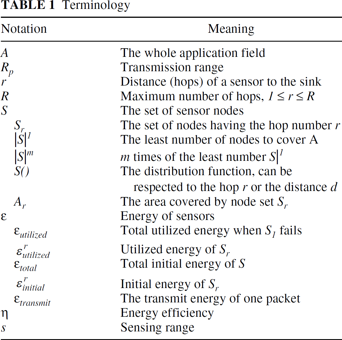
To simplify the analysis, we consider a general model of WSNs while more complex and practical models are left for future work. Suppose a set of independent, homogenous nodes S are distributed to an application field A. We assume A is a circle centered at a single sink. The disk transmission model is valid with a fixed transmission range R_p. Let S_r ⊆ S, 1  r  R denote the set of nodes having the hop count r to the sink (S₁ then contains all the direct neighbors of the sink). |S_r| is the number of nodes in S_r and R represents the maximum number of hops. Let A_r be the area covered by the set S_r. Figure 2 gives an example of the coverage area of S_r. Our final goal is to find the relation or the function between the variable r and S_r. Table 1 lists some of the notations used in this paper. More explanations will be given when these terms are introduced.

Figure 2

Examples of sensing areas of S₁ and S₂.

We assume that a simple routing protocol is available (e.g., GRAB [24]) to provide data delivery service between sensors and the sink. Together with an ideal communication channel, the data is always routed along a single shortest path (the least hop counts) whenever the path exists. A density control algorithm is available (such as PEAS [9]) so that redundant nodes are able to switch to sleep mode when necessary. Note that we are attempting to investigate the impact of node deployment and sink routing-hole problem, not the routing algorithm or the density control mechanism. So we employ one of the most popular ones, while our solution is applicable in conjunction with the other routing protocols. A sensor node consumes two types of energy, ∊_idle and ∊_transmit. ∊_idle is the energy dissipated per second when the sensor is listening to the idle channel or receiving packets. ∊_transmit denotes the energy required per second for packet transmission.

We also have the following approximations.

The consumed energy for idle state is ignored, i.e. ∊_idle = 0;

The energy consumption for the data transmissions originated from the sink is also ignored. Most of the sink-to-sensor transmissions are for queries and commands which should be delivered to all the nodes. Every sensor performs the same amount of tasks. Such operations have less of an impact to the system functionality;

For the sensor-to-sink transmissions, the consumed energy ∊_transmit includes both the reception and transmission operations. Each relay process has just one transmitting and one receiving;

All sensors have the same amount of initial energy;

The amount of data packets sent back to the sink is proportional to the size of the area covered by the sensor; this is for the those periodical monitoring applications; the results can be easily extended to those event-driven applications;

Table 1

Terminology

Notation	Meaning
A	The whole application field
R_p	Transmission range
r	Distance (hops) of a sensor to the sink
R	Maximum number of hops, 1  r  R
S	The set of sensor nodes
S_r	The set of nodes having the hop number r
\|S\|¹	The least number of nodes to cover A
\|S\|^m m	times of the least number S\|¹
S()	The distribution function, can be respected to the hop r or the distance d
A_r	The area covered by node set S_r
∊	Energy of sensors
∊_utilized	Total utilized energy when S₁ fails
∊ ^r _utilized	Utilized energy of S_r
∊_total	Total initial energy of S
∊ ^r _initial	Initial energy of S_r
∊_transmit	The transmit energy of one packet
η	Energy efficiency
s	Sensing range

3.2. The Impact of the Sink Routing-Hole Problem

In this section, we study the sink routing-hole phenomena in uniform distributions. To capture the efficiency of the energy utilization in different scenarios, we define the metric energy efficiency η as:

η = \frac{ε_{u t i l i z e d}}{ε_{t o t a l}} \cdot 100 %

(1)

where ∊_utilized is the used energy when the sink routing-hole appears. ∊_total is the total initialed energy summed up from all nodes.

An ideal case of η = 1 can be achieved when all sensors use up their energy simultaneously as long as the whole network fails. In realistic cases however, it is a challenging job. In the remainder of this subsection, we focus on η of uniform distribution deployment by computing the ∊_utilize and ∊_total respectively.

3.2.1 Total Utilized Energy ∊_utilize

By using the above approximations, we can calculate ∊_utilize as follows.

Let ∊'_utilized,1 < r  R denote the utilized energy of node set S_r when a sink routing-hole is generated (i.e., S₁ fails), then:

ε_{u t i l i z e d} = \sum_{r = 1}^{R} ε_{u t i l i z e d}^{r} .

Following approximation (5), the packet generated by each node is a constant due to the uniform distribution. Suppose each node generates n packets before the sink routing-hole appears. Then for node set S_r, the consumed energy for its own packets is $| S_{r} | \cdot n \cdot ε_{t r a n s m i t}$ , and that for the forwarding services is $\sum_{i = r + 1}^{R} | S_{i} | \cdot n \cdot ε_{t r a n s m i t}$ . Therefore, we have:

\begin{aligned} ε_{u t i l i z e d}^{r} & = | S_{r} | \cdot n \cdot ε_{t r a n s m i t} + \sum_{i = r + 1}^{R} | S_{i} | \cdot n \cdot ε_{t r a n s m i t} \\ = \sum_{i = r}^{R} | S_{i} | \cdot n \cdot ε_{t r a n s m i t} \\ = \frac{R^{2} - (r - 1)^{2}}{R^{2}} \cdot | S | \cdot n \cdot ε_{t r a n s m i t} . \end{aligned}

Thus, ∊_utilized is: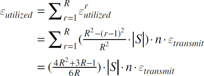

\begin{aligned} ε_{u t i l i z e d} & = \sum_{r = 1}^{R} ε_{u t i l i z e d}^{r} \\ = \sum_{r = 1}^{R} (\frac{R^{2} - (r - 1)^{2}}{R^{2}} \cdot | S |) \cdot n \cdot ε_{t r a n s m i t} \\ = (\frac{4 R^{2} + 3 R - 1}{6 R}) \cdot | S | \cdot n \cdot ε_{t r a n s m i t} \end{aligned}

(2)

3.2.2 Total Initial Energy ∊_total

Assuming sensors have the same amount of initial energy, we have:

ε_{t o t a l} = \frac{| S |}{| S_{1} |} ε_{i n i t i a l}^{1} = R^{2} \cdot ε_{i n i t i a l}^{1}

(3)

where $ε_{i n i t i a l}^{1}$ is the sum of the initial energy is S₁. As S₁ has to support each of the nodes in S to transmit n packets, we have:

ε_{i n i t i a l}^{1} = | S | \cdot n \cdot ε_{t r a n s m i t}

(4)

Recalling the definition of sink routing-hole that S₁ nodes use up all their energy, we have:

ε_{u t i l i z e d}^{1} - ε_{i n i t i a l}^{1} = 0

(5)

Eq. (3), (4) and (5) yield:

ε_{t o t a l} = R^{2} \cdot | S | \cdot n \cdot ε_{t r a n s m i t}

(6)

3.2.3 The Energy Efficiency η

Combining (1), (2), and (6), the energy efficiency of the uniform distributions of deployment is:

\begin{aligned} η & = \frac{ε_{u t i l i z e d}}{ε_{t o t a l}} \cdot 100 % \\ = \frac{4 R^{2} + 3 R - 1}{6 R^{3}} \cdot 100 % \end{aligned}

(7)

Figure 3 depicts the Eq. (7) the function of η over the size of field R. For a relatively small target area with R = 5, only less than 16% of the energy is used before the system is down. With the field increased, the problem becomes more serious. For a field with a maximum of 35 hops, when the network fails, no more than 2% of the total energy has been used. Obviously, the sink routing-hole problem dramatically deteriorates the usability and service quality of WSNs. It becomes the bottleneck of the network lifetime. The random and uniform distribution function is not suitable for WSNs.

Figure 3

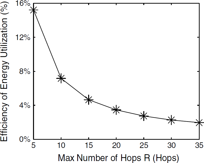
The energy efficiency of uniform distribution.

3.3. Optimal Distribution Function S(r)

To prevent the sink routing-hole from happening, we propose a non-uniform, power-aware node deployment. The key issue is the number of nodes associated with the distance to the sink. More specifically, we are interested in the node deployment function S(r) = |S_r| where r is the hop distance to the sink.

The optimal solution comes from the expectation that all the nodes in sets S_r deplete their energy simultaneously. Therefore, they lose their coverage and connectivity at the same time. For each set S_r, it must carry enough energy to relay the packets of set S_{r +
1} and to transmit its own sensing data. That is:

ε_{i n i t i a l}^{r} = ε_{i n i t i a l}^{r + 1} + c A_{r}

where c represents a constant so that cA_r denotes the energy cost of its own data transmissions. For the farthest set S_R, there is no relay request and all the energy is for sensory data, i.e.,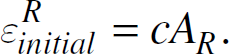

ε_{i n i t i a l}^{R} = c A_{R} .

Let ∊ represent the initial energy of individual sensors, we then have: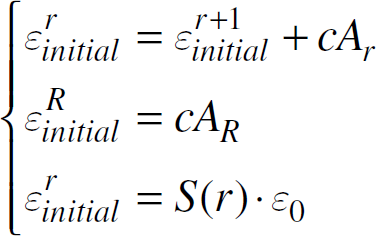

{\begin{cases} ε_{i n i t i a l}^{r} = ε_{i n i t i a l}^{r + 1} + c A_{r} \\ ε_{i n i t i a l}^{R} = c A_{R} \\ ε_{i n i t i a l}^{r} = S (r) \cdot ε_{0} \end{cases}

It yields that:

\begin{aligned} S (r) & = \frac{C}{ε_{0}} \sum_{i = r}^{R} A_{i} = \frac{c \cdot π}{ε_{0}} (R^{2} - (r - 1)^{2}) \\ = \frac{c \cdot π}{ε_{0}} (R^{2} - (r - 1)^{2}) . \end{aligned}

Let c₀ represent all the constant factors and thereby we have:

S (r) = c_{0} \cdot (R^{2} - (r - 1)^{2})

(8)

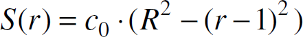
In practice, c₀ is determined by the fact that the total number of nodes is equal to the sum of nodes in sub-areas, i.e.,:

| S | = \sum_{r = 1}^{R} S (r) = \sum_{r = 1}^{R} c_{0} (R^{2} - (r - 1)^{2})

(9)

The parameter |S| in Eq. (9) is the total number of nodes which is known beforehand. The parameter R can be estimated by the size of the field and the transmission range R_P. With c₀ determined by Eq. (9), S(r) is achieved by Eq. (8) to guide the deployment.

3.4. Practical Issues and the Removal of Unit Disk Model

In the previous section, we assume that the unit-disk model is valid. However, the unit-disk model is unlikely to be effective. Many recent experimental studies [25, 26] have shown that wireless links can be highly unreliable. So this issue must be taken into consideration in the design of protocols.

The promising nature of the power-aware deployment is that the distribution function $S (r) = c_{0} \cdot (R^{2} - (r - 1)^{2})$ can be applied with the continuous distance d, although it can be achieved from the assumption of a discrete communication function. It does not require the unit-disk model and can be employed to the realistic environments without significant changes.

In general cases where d > R_P, the distribution function is $S (d) = c_{0} \cdot (R^{2} - (\frac{d}{R_{P}} - 1)^{2})$ . To examine the correctness and system errors of this approximatıon, we need to compare the non-continuous function S(r) with the continuous function S(d). For the former function S(r), given two boundaries of hops r₂  r₁  1, the node set S_r, r₂  r  r₁ has the following number of nodes:

\begin{aligned} | S_{r} | & = \sum_{r = r_{1}}^{r_{2}} (c_{0} \cdot (R^{2} - (r - 1)^{2})) \\ = c_{0} \cdot (R^{2} (r_{2} - r_{1}) - \frac{(r_{2} - r_{1})^{3}}{3} - \frac{(r_{2} - r_{1})^{2}}{2} - \frac{(r_{2} - r_{1})}{6}) \end{aligned}

(10)

For the latter function S(d), the node set $S_{d}, r_{2} \geq \frac{d}{R_{P}} \geq r_{1}$ has the following number of nodes:

\begin{aligned} | S_{r} | & = \int_{d = r_{1} \cdot R_{p}}^{r_{2} \cdot R_{p}} c_{0} \cdot (R^{2} - (\frac{d}{R_{p}} - 1)^{2}) \\ = c_{0} \cdot (R^{2} (r_{2} - r_{1}) - \frac{(r_{2} - r_{1})^{3}}{3}) \end{aligned}

(11)

It is encouraging to discover that (10) and (11) have differences in minor terms only. The different portions (r₂ – r₁)² and (r₂ – r₁) have lower orders than (r₂ – r₁)³, implying that they can be ignored.

For the special case d  R_p, nodes are actually direct neighbors of the sink. It is sufficient to uniformly distribute the number $| S_{1} | = c_{0} \cdot R^{2}$ of nodes around the sink so that the continuous function S(r) and non-continuous function S(d) have the same output in the corresponding domain.

4. Performance Evaluation

In this section, we investigate power-aware node deployment by simulation. We first define the evaluation metrics, and then introduce the experimental setup. In the end we show the simulation results.

4.1. Performance Metrics

Although the network lifetime is one of the most critical of issues, it is difficult to give a unique definition of lifetime in the context of WSNs. The definitions from MANET are not suitable for WSNs. Instead, we use the metric coverage rate λ defined as:

λ = \frac{A_{sin k}}{A} \cdot 100 %,

where A_sink denotes the area covered by sensors which are reachable from the sink through multi-hop routing. We should note that A_sink is different from A_active which represents the area covered by all the active nodes. Some nodes may be active but its packet can never be routed to the sink due to the lack of intermediate nodes. These area variables have the relation that $A_{s i n k} \leq A_{a c t i v e} . \leq A$ .

We are also interested in the quality of data delivery services. We define success rate κ as:

κ = (\frac{P a c k e t_{t o_sin k}}{P a c k e t_{a l l}}) \cdot 100 %,

where Packet_{to_sin k} is the cumulative number of packets successfully delivered to the sink, and Packet_all is the total number of generated data packets. We have Packet_{to_sink}  Packet_all because packets may be dropped due to the failure of intermediate forwarding nodes. We apply a single-path routing algorithm. Although multi-path routing algorithms [4, 24, 27] may increase the transmission reliability and hence the success rate, they consume more energy of S₁ for each data. This will always make the sink routing-hole problem even more serious.

4.2. Experiment Setup

We have implemented GRAB and PEAS in our simulators as the routing protocol and the density control mechanism. Figures 4 and 5 illustrate examples of the uniform distribution and power-aware deployment with a maximum of 5 hops away from the sink.

Figure 4

An example of uniformed distribution.

Figure 5

An example of power-aware distribution.

To determine the number of nodes that should be distributed, we assume that sensors are deployed with a “high density.” The total number of nodes is several times of the least required number of nodes to cover the field |S| ¹ . To determine |S| ¹ , we approximate the sensing area of the individual node as a hexagonal shape so that the sensors could fully cover A. To simplify our presentation, we assume the sensing range s is the same as the transmission range R_p. Since sensing area being tangent to each other is not enough to cover the whole field—some area between disks is not covered—we apply the hexagonous shape of sensing domain as the approximation of the circle sensing area (as shown in Fig. 6). Accordingly, |S| ¹ can be calculated by: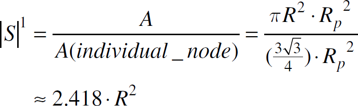

\begin{aligned} | S |^{1} & = \frac{A}{A (i n d i v i d u a l_n o d e)} = \frac{π R^{2} \cdot {R_{p}}^{2}}{(\frac{3 \sqrt{3}}{4}) \cdot {R_{p}}^{2}} \\ \approx 2.418 \cdot R^{2} \end{aligned}

(12)

Figure 6

Hexagon shaped sensing area.

In addition, let |S| ^m ,m  1 denote m times the least number of $| S |^{l}, i . e ., | S |^{m} = m \cdot | S |^{l}$ .

We select sensor hardware parameters similar to that of Berkeley Motes [28]. The power consumptions in transmission and reception are 60mW and 12mW, respectively. The active and sleep modes have the power consumption of 12mW and 0.03mW, respectively. The initial energy of a node is 30 joules, which allows a sensor to work for more than 2500 seconds when there is no data transmission or sleeping. The transmission range is set to be 10 meters. Each node initiates a data report per second.

4.3. Simulation Results

In this subsection, we will show some simulation results. We will compare the power-aware deployment with uniform distribution with respect to scalability and node density.

4.3.1 Performance with Different Network Scales

To deploy sensors with relatively high density, a |S| ⁵ number of nodes are distributed to the field. We first compare power-aware deployment with uniform distribution with varied field size of radii 50, 100, and 200 meters, respectively. There are 250, 750, and 2500 nodes, respectively. Figures 7 to 12 show the performance.

Figure 7

Coverage ratio of power-aware and uniform distributions with 250 nodes.

Figure 8

Coverage ratio of power-aware and uniform distributions with 750 nodes.

Figure 9

Coverage ratio of power-aware and uniform distributions with 2500 nodes.

Figure 10

Success rate of power-aware and uniform distributions with 250 nodes.

Figure 11

Success rate of power-aware and uniform distributions with 750 nodes.

Figure 12

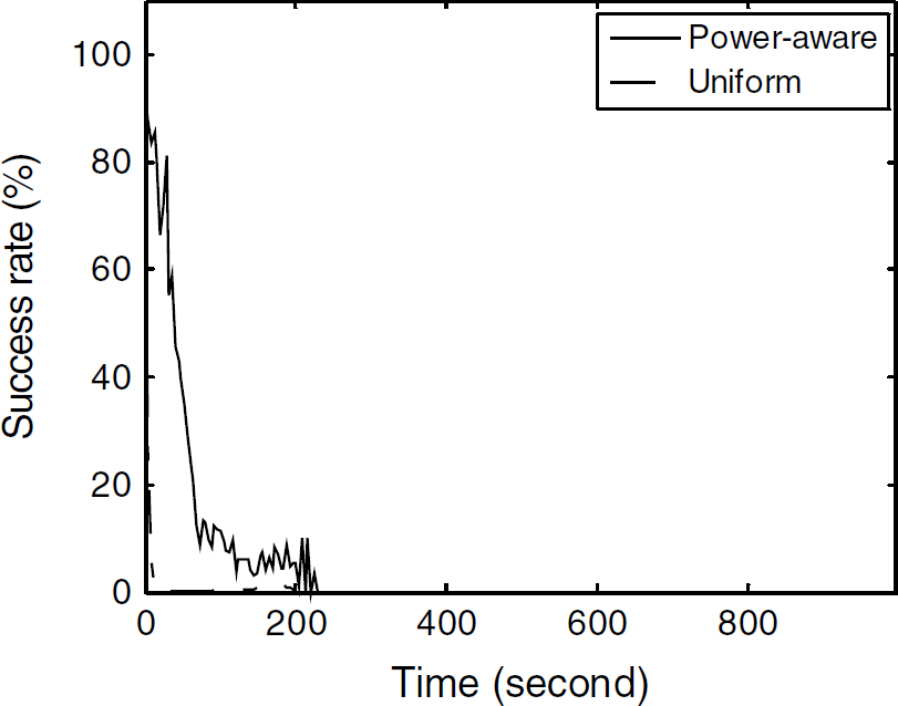
Success rate of power-aware and uniform distributions with 2500 nodes.

Figures 7 to 9 depict the coverage rates of power-aware distribution and uniform distribution. The graphs show that the coverage rate of the uniform distribution drops sharply at the very beginning. Most sensors are disconnected from the sink after 5 to 20 seconds. In contrast, the power-aware deployment greatly improves the network connectivity. The system has operated for 20 to 100 seconds in the corresponding network size with a relatively high coverage rate. In a larger field, the improvement of power-aware deployment is more. For the uniform distribution, the number of sensors increases while the node density around the sink remains a constant. The nodes of S₁ have the heavier workload and their energy is consumed faster as the field size expands. In power-aware distribution, more nodes are placed near the sink which results in sufficient energy distribution for greater demand of packet forwarding.

Figures 10 to 12 show the performance in terms of the success rate. For both distributions, the success rate drops when the coverage area increases. The major reason is that the packet transmission is more likely to be interrupted by a single node failure as the number of hops increases. Power-aware deployment has enough redundant nodes near the sink. Thus it presents an average success rate much higher than the uniform distributed does.

This set of experiments shows that power-aware distribution is more scalable than the uniform distribution does in terms of the coverage rate and data success rate.

4.3.2 Performance with Different Node Densities

In this set of experiments, we will evaluate the scalability of power-aware deployment and the uniform distribution with different node densities. The density varies as |S|³, |S| ⁴ and |S| ⁵ , and the results are shown in Figures 13 to 16.

Figure 13

Coverage ratio of power-aware deployment with 500, 750, 1000, 1500, 2000, and 2500 nodes.

Figure 14

Coverage ratio of uniform deployment with 500, 750, 1000, 1500, 2000, and 2500 nodes.

Figure 15

Success rate of power-aware deployment with 500, 750, 1000, 1500, 2000, and 2500 nodes.

Figure 16

Success rate of uniform deployment with 500, 750, 1000, 1500, 2000, and 2500 nodes.

Figures 13 and 14 show that node density can significantly increase the network coverage ratio under power-aware distribution. For example, for the 500-node configuration, λ reduces to about 50% after 100 seconds. And for the configuration of 2500 nodes, it is increased to 400 seconds. This result conforms the fundamental design philosophy of WSNs that to increase the network functionality by a higher density and more deployment of nodes. For uniform distribution, more nodes make the coverage ratio decrease. It contradicts the design philosophy and thus is not acceptable. Figures 15 and 16 give a similar result. For the transmission success rate κ, under power-aware deployment, most of the data packets can be successfully delivered until most of the nodes deplete their energy. For the case of uniform distribution, however, most of the packets are lost since the very beginning. This result implies that when uniform distribution is applied, it may not be a good solution to improve the network lifetime by increasing the number of deployed sensors. More nodes deployed to the field will result in an even earlier occurrence of the network malfunction.

5. Conclusions and Future Work

In this paper, we attempted to answer a practical question as to how we should deploy sensors to an application field. By investigating the sink routing-hole phenomenon, we pointed out the main weakness of the random and uniform deployment. Accordingly, we proposed a non-uniform, power-aware deployment scheme based on a general sensor application model. The power-aware deployment is optimized to maintain a continuous connectivity-coverage instead of that for some particular snapshots of the network. Theoretical analysis and simulation results have shown that power-aware deployment can dramatically increase the network lifetime and improve the network service quality.

In our future work, we have mainly two directions. One is to extend our work to more complicated and specific models. Currently, our power-aware deployment scheme is derived from a simple and generic model, where the target territory is a circle centered at a single sink. We shall investigate optimal deployment schemes for other models, including the fields having irregular shapes, the sink being positioned on different places, and the scenarios with multiple sinks. The other is to extend our power-aware deployment from maintaining the connectivity coverage to provide a long-term continuous sensing coverage, which is more concerned by end users.

Footnotes

Acknowledgement

This research was supported in part by Hong Kong RGC Grant HKUST6183/05E, the Key Project of China NSFC Grant 60533110, and the National Basic Research Program of China (973 Program) under Grant No. 2006CB303000.

References

Culler

Estrin

Srivastava

, “Sensor Network Applications,” IEEE Computer, 41–78, 2004.

Xue

Luo

Chen

Liu

, “Contour Map Matching For Event Detection in Sensor Networks,” in Proceedings of SIGMOD, to appear, 2006.

Akyildiz

I. F.

Sankarasubramaniam

Cayirci

, “A Survey on Sensor Networks,” IEEE Communications Magazine, vol. 40, 102–114, 2002.

Raghunathan

Schurgers

Park

Srivastava

M. B.

, “Energy-aware Wireless Microsensor Networks,” Signal Processing Magazine, vol. 19, 40–50, 2002.

Corke

Hrabarz

Petersony

Rusyx

Saripalliz

Sukhatme

, “Autonomous Deployment and Repair of a Sensor Network using an Unmanned Aerial Vehicle,” in Proceedings of IEEE International Conference on Robotics and Automation (ICRA), 2004.

Luo

Cheng

Zhang

, “A Two Tier Data Dissemination Model for Largescale Wireless Sensor Networks,” in Proceedings of ACM MobiCom, 2002.

Petrovic

Shah

R. C.

Ramchandran

Rabaey

, “Data Funneling: Routing with aggregation and compression for wireless sensor networks,” in Proceedings of IEEE Sensor Network Protocols and Applications (SNPA), 2003.

Berman

Calinescu

Shah

Zelikovsky

, “Power Efficient Monitoring Schedules in Sensor Networks,” in Proceedings of IEEE Wireless Communication and Networking Conference, 2004.

Zhong

Cheng

Zhang

, “PEAS: A Robust Energy conserving Protocol for Long-lived Sensor Networks,” in Proceedings of ICDCS, 2003.

10.

Zhang

Hou

J. C.

, “Maintaining Coverage and Connectivety in Large Sensor Networks,” The Wireless Ad Hoc and Sensor Networks: An International Journal, 2005.

11.

Liu

Lun

R. N. H.

L. M.

, “Power-aware Node Deployment in Wireless Sensor Networks,” in Proceedings of International Conference on Sensor Networks, Ubiquitous, and Trustworthy Computing (SUTC), 2006.

12.

Bogdanov

Maneva

Riesenfeld

, “Power-asware Base Station Positioning,” in Proceedings of INFOCOM, 2004.

13.

Wang

Cao

Porta

T. L.

Zhang

, “Sensor Relocation in Mobile Sensor Networks,” in Proceedings of INFOCOM, 2005.

14.

Yang

, “SMART: A Scan-Based Movement-Assisted Sensor Deployment Method in Wireless Sensor Networks,” in Proceedings of INFOCOM, 2005.

15.

Sankar

Liu

, “Maximum Lifetime Routing in Wireless Ad-hoc Networks,” in Proceedings of INFOCOM, 2004.

16.

Wang

Xiao

Liu

Zheng

, “Distributed Caching and Adaptive Search in Multilayer P2P Networks,” in Proceedings of ICDCS, 2004.

17.

Chen

Jamieson

Balakrishnan

Morris

, “SPAN: An energy Efficient Coordination Algorithm for Topology Manitenance in Ad Hoc Wireless,” in Proceedings of MOBICOM, 2001.

18.

Cerpa

Estrin

, “Ascent: Adaptive self-configuring sensor networks topologyies,” in Proceedings of INFOCOM, 2002.

19.

Liu

Xiao

L. M.

Zhang

, “Location-Aware Topology Matching in P2P Systems,” in Proceedings of INFOCOM, 2004.

20.

Wei

Srinivasan

Chaing

C. K.

, “Using Mobile Relays to Prolong the Lifetime of Wireless Sensor Networks,” in Proceedings of MobiCom, 2005.

21.

L. M.

Liu

Lau

Y. C.

Patil

A. P.

, “LANDMARC: Indoor Location Sensing Using Active RFID,” in Proceedings of PerCom, 2003.

22.

Liu

Zhuang

Xiao

L. M.

, “Distributed Approach to Solving Overlay Mismatching Problem,” in Proceedings of ICDCS, 2004.

23.

Zhang

Nygard

, “Improving Coverage ZPerformance in Sensor Networks by Using Mobile Sensors,” in Proceedings of MILCOM, 2005.

24.

Zhong

Zhang

, “GRAdient Broadcast: A Robust Data Delivery Protocol for Large Scale Sens or Networks,” ACM Wireless Networks, vol. 11, 285–298, 2003.

25.

Couto

D. S. J. D.

Aguayo

Bicket

Morris

, “A High-Throughput Path Metric for Multi-Hop Wireless Routing,” in Proceedings of ACM MobiCom, 2003.

26.

Zhao

Govindan

, “Understanding Packet Delivery Performance in Dense Wireless Sensor Networks,” in Proceedings of ACM Sensys, 2003.

27.

Ganesan

Govindan

Shenker

Estrin

, “Highly-resilient, Energy-efficient Multipath Routing in Wireless Sensor Networks,” in Proceedings of ACM MobiCom, 2001.

28.

Hill

Szewczyk

Woo

Hollar

Culler

Pister

, “System Architecture Directions for networked Sensors,” in Proceedings of International Conference on Architectureal Support for Programming Languages and Operating Systems(ASPLOX-IX), 2000.

Power-Aware Node Deployment in Wireless Sensor Networks

Abstract

Keywords

1. Introduction

3. Analysis of Sink Routing-Hole Phenomenon

3.1. Concepts and Terminologies

4.1. Performance Metrics

4.2. Experiment Setup

4.3.1 Performance with Different Network Scales

Footnotes

Acknowledgement

References