Sage Journals: Discover world-class research

Abstract

Dynamic network is an abstraction of networks with frequent topology changes arising from node mobility or other reasons. In this article, we first propose a dynamic network model, named (T, L)-HiNet, to extend existing dynamic network models with clusters. (T, L)-HiNet includes several properties defining the stability of cluster hierarchy in a dynamic network, including cluster head set, cluster member set and the connections among them. Based on (T, L)-HiNet, we design several hierarchical information dissemination algorithms for different scenarios of dynamics. Furthermore, we extend the (T, L)-HiNet model and corresponding algorithms in two directions, that is, stability of cluster head set and cluster size. The correctness of our algorithms is proved rigorously, and their performance is evaluated via both numerical analysis and simulations. The results show that compared with the algorithm recently proposed by Kuhn et al., our design can significantly reduce communication cost and also time cost.

Keywords

Information dissemination dynamic network cluster distributed algorithm system model

Introduction

Due to node mobility and other reasons, the topology of a computer network, for example, wireless ad hoc network or a peer-to-peer (P2P) overlay network, may change frequently from time to time. Dynamic network is the general abstraction of such networks with formalized network models.^1,2 Based on these models, various communication and computation problems can be addressed with formally proved correctness,^3,4 which is basically different from practical work.^5,6

Information dissemination is one of such problems, where the network nodes need to disseminate information throughout the network.^7,8 It can be defined as the k-token dissemination problem,^9,10 where each node receives an initial set of tokens drawn from some domain, such that the total number of tokens in the input to all nodes is k. The goal is for each node to collect and output all k tokens.

In dynamic network, a message is only propagated from the node to all others hop by hop, without using routing algorithm.⁶ Due to unceasing change and limited connection, information dissemination in dynamic network is a challenging task. With different dynamics models, quite a number of algorithms^9–13 have been designed for this problem. Almost all these works focus on how to propagate information fast against topology changes, and another important issue, communication cost has been largely ignored. Communication cost in distributed computation, that is, the cost to send and receive packets, is crucial in many instances of dynamic networks, for example, mobile ad hoc networks, wireless sensor networks, and vehicular ad hoc network.^14,15

This motivates us to pursue communication efficiency in information dissemination in dynamic networks. Basically, we introduce clusters into dynamic networks and make use of the cluster-based hierarchy to reduce transmissions conducted. Clustering has been widely studied and adopted in ad hoc networks to reduce communication cost and improve scalability in various networking and application problems.^16–19

However, making use of cluster hierarchy in dynamic networks is a challenging task. First, hierarchy makes the network architecture more complex, and it will change with the network topology changes. Therefore, more dynamic factors need to be modeled and defined. Second, with hierarchy, the upper layer algorithms, like information dissemination algorithms, must operate differently at ordinary nodes and cluster head nodes, which are obviously more complex than those based on a flat architecture, that is, network without hierarchy via clustering or predefined backbone nodes.

In this article, we first propose a new dynamic network model, called (T, L)-HiNet, which extends existing models by including cluster hierarchy. The key point lies in the definition of different stability properties to model the dynamics of the hierarchy, including set of cluster heads, set of members in a cluster, and connectivity among cluster heads. Based on (T, L)-HiNet, we design information dissemination algorithms for different scenarios of dynamics. All the algorithms make use of clusters to reduce communication cost. Clusters can also help speed up the procedure of information dissemination if the hierarchy is stable enough.

Then, we extend the (T, L)-HiNet model in two directions. First, we consider the scenario of ∞-interval stable cluster head set. Interestingly, with such a stable cluster head set, information dissemination can be conducted without constraining the behavior of cluster members. Correspondingly, we extend our algorithms for (T, L)-HiNet to the network of ∞-interval stable cluster head set. Second, we extend (T, L)-HiNet from one-hop clustering to multi-hop clustering and define a new hierarchical dynamic network model (T, L, D)-HiNet. Correspondingly, the information dissemination algorithms for one-hop clustering networks are extended to handle multi-hop clusters.

All our proposed algorithms are proved to be correct in terms of information delivery. Moreover, we evaluate the performance of them via both numerical analysis and simulations, in terms of both communication cost and time cost. The algorithm recently proposed by Kuhn et al.⁹ is chosen for comparison purpose. The results confirm the benefit of our design very well.

The rest of the article is organized as follows. Section “Related work” briefly reviews existing work on dynamic networks, including both network models and information dissemination algorithms. We describe our new dynamic network model (T, L)-HiNet in section “(T, L)-HiNet: a hierarchical dynamic network model,” including the basic system model describing the underlying environment, the cluster-based time-varying graph (CTVG) graph model to represent the hierarchical network, and the stability properties to model dynamics of the hierarchy. In section “Hierarchical information dissemination algorithms,” we describe our hierarchical information dissemination algorithms and prove their correctness. Two extensions to the (T, L)-HiNet model and the corresponding modifications in information dissemination algorithms are presented in section “Extensions to (T, L)-HiNet.” Performance evaluations via numerical analysis and simulations are reported in sections “Performance comparison and analysis” and “Simulation results,” respectively. Finally, section “Conclusion and future work” concludes the article with future directions.

Related work

Network model is the basis of dynamic network study. Dynamic network models are usually defined by extending graph models for general networks and the key point is how to reflect the dynamics of the network topology. Existing models define network topology changes from two different points of view, that is, edge-centric models and graph-centric models. Edge-centric models focus on the changes of edges against time, that is, edges may appear or disappear and consequently cause topology changes. Graph-centric models concern more about the overall properties in the graph level, such as connectivity, diameter.

Edge-centric models can be found in the literatures.^1,4,20,21 Kempe et al.¹ proposed the temporal network (G, λ), where λ is a time labeling of G specifying the time at which the edge e is available. Akrida et al.²¹ studied the temporal diameter of the directed random temporal graph model for the case of r = n. Clementi et al.²⁰ have introduced the notion of edge-Markovian dynamic graph (EMDG), which refers to stochastic edge time-dependency in evolving graphs. Leskovec et al.⁴ propose an edge-centric model, which views a dynamic network as a sequence of static graphs. Avin et al.²² consider that topology changes only occur once within every certain number of rounds.

Graph-centric models are proposed in Kuhn and colleagues.^3,9 The notion of dynamic diameter is proposed by Kuhn and Oshman,³ which is a bound on the time required for each node to be causally influenced by each other node. The dynamic diameter extends the concept of normal diameter of a graph with consideration of dynamic changes. Kuhn et al.⁹ propose the T-interval connected model, which stipulates that for every T consecutive rounds, there exists a stable connected spanning subgraph. In our previous work,²³ we proposed (Q, S)-distance model, which is used to describe dynamic changes of information propagation time between any two nodes. Ducourthial and Wade²⁴ introduce a dynamic p-graphs model. The model constitutes a finite set of dynamic graphs, with the particularity that their edges allow transferring p messages.

Time-varying graph (TVG)²⁵ is a general dynamic network model, which integrates previous models with a unified framework. With TVG, a dynamic network is modeled as G = (V, E, T, ρ, ζ), where V and E are the vertex and edges in the topology graph, respectively, T is the lifetime of the network, ρ indicates whether a given edge is available, and ζ represents the time taken to cross an edge. Wehmuth et al.²⁶ propose a new unifying model for representing finite discrete TVGs, which can capture the needs of distinct dynamic networks. These two models can switch between graph-centric and edge-centric perspectives on the dynamics. All these models consider flat network architecture. To reflect cluster-based hierarchies in a dynamic network, new models are necessary.

Information dissemination was first studied in the static networks.¹¹ In a static graph network, k-token dissemination¹³ can be completed in time O(n + k) via flooding, where n is the total number of nodes. Gossiping is a commonly used probabilistic approach to information dissemination in static environments,^27–30 where each node chooses one or a few nodes at random in each round to exchange information with them. Kempe et al.²⁸ use gossip-style local communication to provide simple and fault-tolerant protocols. Mosk-Aoyama and Shah²⁷ consider a randomized gossip mechanism for information dissemination.

Information dissemination in dynamic networks is usually realized by flooding or similar approaches,^2,4,12,31,32 which is necessary to theoretically guarantee the delivery of information to all nodes. The algorithm proposed by Clementi et al.²⁰ is based on the EMDG model with consideration of edge birth rate and death rate. Baumann et al.¹² proposed the k-active flooding protocol, where each node will forward information received for k times so as to speed up the propagation of information. Sarma et al.³³ introduce distributed random walk algorithms in dynamic networks. Augustine et al.³⁴ propose a centralized algorithm that completes gossip in O(n^3/2) rounds with high probability, under any oblivious adversary. Michail et al.³⁵ study the propagation of influence and computation in dynamic networks that are possibly disconnected at every instant. They propose a set of minimal temporal connectivity conditions, which require that another causal influence occurs within every time window of some given length.

Kuhn et al.⁹ studied information dissemination from the view of network connectivity. They show that one piece of information (i.e. one token) can be disseminated with guaranteed delivery to the whole network once the underlying network is connected at any time. This has been proved to be the weakest requirement for information dissemination in dynamic networks. Kuhn et al.⁹ studied k-token dissemination based on the T-interval connectivity model. Following this conclusion in Kuhn et al.,⁹ one-token dissemination can be correctly completed via flooding in one-interval connected networks in n – 1 rounds. They design algorithms for general case of T-interval connected networks and show that the computation can be sped up by factor T compared with one-interval connected networks. Haeupler and Karger¹⁰ improved the work in Kuhn et al.⁹ by making use of network coding to speed up the procedure of disseminating.

All the above information dissemination algorithms focus on how to guarantee the correctness of information delivery. Since real deployed dynamic networks, like mobile ad hoc networks or wireless sensor networks, are resource constrained, how to achieve information dissemination with guaranteed correctness and low cost is obviously significant. This motivates us to design communication efficient algorithms by making use of cluster-based hierarchy.

(T, L)-HiNet: a hierarchical dynamic network model

(T, L)-HiNet is a new model of dynamic networks, which includes cluster hierarchy. In the following, we first describe the system model, which includes basic assumptions on the underlying network and clusters. The core part is the definition of (T, L)-HiNet, a model of the stability properties of cluster-based hierarchy. We also define a graph model CTVG, which is used in the definition of (T, L)-HiNet to represent the underlying network.

System model

We consider an ad hoc network with a set of nodes, each of which has a unique identifier. The network nodes communicate with each other via multi-hop paths. The neighborhood among network nodes is determined by the communication range of the wireless transmission. Each node is equipped with the capability of probing neighbors. The network runs in synchronized rounds and the time can be denoted by {t₀, t₁,.., t_i,…}, where [t_i, t_i_+ 1) is one round. In every round, each node u generates a message to be delivered to all its current neighbors and its neighbors can receive the message at current round. The topology of network may change from time to time, due to node mobility or other reasons.

A cluster-based hierarchy is constructed by clustering nodes into clusters. Since the network topology changes from time, the cluster-based hierarchy will change accordingly and re-clustering is possible. The clustering procedure can be carried out by clustering algorithms, which is out of the scope of this article. We just assume the existence of such hierarchy, with following characteristics.

Each node belongs to at most one cluster at any given time but it may change its cluster from time to time. There is one and only one cluster head in each cluster and each cluster has a unique cluster identifier. For simplicity of presentation, the node ID of cluster head is used as the cluster ID in this article. The members of a cluster are neighbors of the cluster head and obviously, they know each other. Cluster heads may be connected via gateway nodes selected by clustering algorithms. Figure 1 shows an example network with cluster-based hierarchy constructed.

Figure 1.

An example network with clusters.

Definition of CTVG

Now, we define the new dynamic network model CTVG, which is the extension of TVG with cluster-based hierarchy.

Definition 1

(Cluster-based time-varying graph, CTVG): G = (V, E, Γ, ρ, ζ, C, I), where

V: the set of nodes that are present in the network.

E ⊆ V × V × L, the edge matrix represents the relationship between the nodes. L stands for some property associated with edges, such as the bandwidth of a link.

Γ: lifetime of the system. Γ is divided into consecutive rounds; each round presents one send/receive time.

ρ: E × Γ → {0, 1}, the presence function indicating whether a given edge is available at a given time.

ζ: E × Γ → Γ, the latency function representing the time taken to cross an edge.

The above elements have been defined in the TVG model. To represent clusters, we introduce two new elements C and I. C is used to represent what status of the node in cluster and I is used to represent which cluster the node belongs to.

C: V × Γ → {h, g, m}, the status of each node at a given time. The meaning of the status value: h indicates that the node is a cluster head; g indicates that the node is a cluster gateway node and responsible for forwarding packets between clusters; m indicates that this node is a common node, that is, a cluster member.

I: V × Γ → N, the cluster that each node belongs to at a given time. N is the ID of the cluster.

With the definition above, a dynamic network with clusters can be clearly represented by CTVG. In a dynamic network, the network topology and the cluster structure will change from time to time. Therefore, we need to model the dynamics of the cluster-based hierarchy, that is, how the hierarchy will change against time.

Definition of (T, L)-HiNet

We model the dynamics of cluster-based hierarchy in terms of how the hierarchy keeps stable. The following notions may be used in our dynamic models:

$V_{h}^{i}$ : the set of cluster head nodes in the time[t_i, t_i_+ 1), where $V_{h}^{i} \subseteq V$ and $\forall v \in V, C (v, i) = h \Leftrightarrow v \in V_{h}^{i}$ .

$M_{k}^{i}$ : the cluster member set of cluster k in time [t_i, t_i_+ 1), where $M_{k}^{i} \in V$ and $\forall v \in V, I (v, i) = k \Leftrightarrow v \in M_{k}^{i}$ .

To model the dynamics of cluster-based hierarchy, that is, the changes of clusters, we define the following stability properties. Basically, we borrow the concept of T-interval from Kuhn et al.,⁹ to define the stability of clusters. T-interval denotes every T consecutive rounds. T can be any number, from 1 to ∞.

Definition 2

(T-interval stable cluster head set, T_s): We say the cluster head set is T-interval stable that

\forall c \in N, \forall i, j \in [c^{*} T, c^{*} T - 1) \Rightarrow V_{h}^{i} = V_{h}^{j}

This property requires that the set of cluster head keeps unchanged during the T-interval time. Obviously, the larger the T is, the more stable the cluster head set is. Especially, an ∞-interval stable cluster head set can be constructed using some special cluster head nodes as in Ng et al.¹⁸

Definition 3

(T-interval stable cluster, T_c): We say a cluster k is T-interval stable that

\forall c \in N, \forall i, j \in [c^{*} T, c^{*} T - 1) \Rightarrow M_{k}^{i} = M_{k}^{j}

Definition 4

(T-interval stable hierarchy, T_h): We say the cluster-based hierarchy is T-interval stable that the structure of hierarchy keeps unchanged in T-interval time that

\begin{matrix} \forall k \in N, \forall c \in N, \forall i, j \in [c^{*} T, c^{*} T - 1) \\ \Rightarrow V_{h}^{i} = V_{h}^{j} and M_{k}^{i} = M_{k}^{j} \end{matrix}

Obviously, in a T-interval stable hierarchy, the cluster head set must be T-interval stable (Definition 2) and all the clusters are T-interval stable (Definition 3).

Definition 5

(T-interval cluster head connectivity, T_d, and T-interval cluster head subgraph, $ϒ$ ): We say a dynamic network has T-interval cluster head connectivity if $\forall i \in N, \exists ϒ \subseteq G_{i} : V_{ϒ} \supseteq V_{h}^{i}$ , $ϒ$ is connected, and $\forall j \in [i, i + T - 1), ϒ \subseteq G_{j}$ .

Accordingly, the subgraph $ϒ$ is called T-interval cluster head subgraph.

Definition 6

(L-hop cluster head connectivity): We say that the connectivity among cluster heads is L-hop if

\min {L | \forall S \subset V_{h}^{i}, v \in V_{h}^{i} \ S, a n d \exists u \in S, d i s t a n c e (u, v) \leq L}

L in fact indicates the maximum value of the shortest path between any two cluster heads that connected directly or by only gateway nodes. This is a key parameter that affects the procedure of information dissemination, as shown later in algorithm design and analysis.

L can be delicately controlled by clustering algorithms, as in weakly connected dominating set (WCDS)-based clusters.^14,15 Interestingly, in a one-hop cluster-based network as assumed in our system, the value of L is not more than three.

Definition 7

(T-interval L-hop cluster head connectivity): The cluster-based hierarchy is with both T-interval cluster head connectivity and L-hop cluster head connectivity in the subgraph $ϒ$ .

Definition 8

(T-interval L-hop Hierarchy Network, (T, L)-HiNet): a dynamic network with T-interval stable hierarchy (Definition 4), and T-interval L-hop cluster head connectivity (Definition 7) is called a T-interval L-hop hierarchical network, denoted by (T, L)-HiNet.

The seven definitions above describe the dynamics of a cluster-based hierarchy from different points. Figure 2 shows the relationship among the definitions by a tree structure, where a higher level definition is the combination of its children ones in the lower level.

Figure 2.

Relationship among definitions.

Hierarchical information dissemination algorithms

Based on the (T, L)-HiNet model defined in the previous section, we design two algorithms for hierarchical information dissemination. The first algorithm is for the general case of (T, L)-HiNet, while the second algorithm is for (1, L)-HiNet. (1, L)-HiNet is the worst case of (T, L)-HiNet because only one-interval connectivity is guaranteed. Both the algorithms are proved to be correct with respect to token information delivery.

With the example scenario shown in Figure 3, we briefly describe the basic procedure to help the understanding of our algorithms later. When a node u wants to disseminate the token t, it will send t to its cluster head v. Then node v sends token t to all its neighbor nodes via broadcasting. When a gateway node receives token t, it will further propagate t by sending it toward other clusters. When another cluster head w receives token t, it will broadcast the token to all neighbors as v has done. To guarantee that the token will be delivered to all nodes, each cluster head with token t will broadcast the token once in each T rounds. A cluster head can stop broadcasting t after a specific number of time intervals, which is necessary to guarantee that t will be delivered to all nodes. The number of time intervals needed will be discussed in the algorithm operations.

Figure 3.

An example illustration of Algorithm 1.

The algorithm for (T, L)-HiNet

Description of algorithm operations

To disseminate k tokens, the procedure is divided into M phases, each consisting of T rounds. The value of M will be discussed later. According to the role of a node, that is, member, cluster head, or gateway, different operations are executed. The pseudo code of the algorithm is shown in Figure 4.

Figure 4.

The algorithm for (T, L)-HiNet.

Each node needs to maintain three sets. TA is the set of tokens ever collected; TS is set of tokens broadcast by the node in the current phase; and TR is the set of tokens received from the current cluster head. Each token is stamped with a unique id, and the id is comparable with others.

Each member node u executes the algorithm with M phases. In the beginning of each phase, node u needs to check whether its cluster head has been changed. If its cluster head is different from the one in previous phase, it needs to empty the two sets: TR and TS. Then u will execute T rounds of operations as follows.

In each round, node u will first check if any token collected have not been known by the current cluster head, that is, TA ≠ TS ∪ TR. Then, node u sends token t to the current cluster head, where token t is with the maximum id that is unknown by cluster head. Token t will be put into TS accordingly.

Node u also needs to receive tokens from its cluster head in each round. Node u updates its token sets TA and TR by adding the token received. Then, one round ends.

The operations at cluster head and gateway nodes are the same. Like cluster members, a cluster head/gateway node executes the algorithms with M phases, and each phase consists of T rounds. In the end of each phase, it needs to empty the set TS.

In each round, a cluster head/gateway needs to first check whether any token has not been sent to its members/neighbors by broadcasting. It will choose token t with the minimum id that has not sent in current phase. The cluster head/gateway updates the set TA by adding the token received and the set TS by adding the token sent. Then, one round ends.

Correctness proof

We now prove the correctness of our hierarchical information dissemination algorithm by showing that each node will have all the k tokens after they finish executing the algorithm. Let dist(u, v) denote the shortest path distance between u and v in the stable subgraph,⁹ we can get Lemma 1.

Lemma 1

For any node v in a round r that dist(v, u) ≤ r ≤ T, either v has collected t or at least (r-dist(v, u)) different tokens.

Proof

This lemma is borrowed from Kuhn et al.,⁹ and we omit its proof.

Lemma 2

With T-interval L-hop cluster head connectivity and T-interval stable hierarchy, for any token t known by node u at the beginning of any phase i, at least $⌊ (T - k) / L ⌋$ cluster head nodes will newly learn t in the end of the phase i.

Proof

Let $N_{i}^{d} (u)$ denote the d-neighborhood of u in phase i. By Lemma 1, for any node $v \in N_{i}^{T - k} (u)$ , either v has collected t or v has k different tokens in round T. Since there are totally k tokens, all nodes in $N_{i}^{T - k} (u)$ have known token t at the end of phase i. Because the clusters are L-hop, and the cluster-based hierarchy has T-interval L-hop cluster head connectivity, at least $⌊ (T - k) / L ⌋$ cluster head nodes are in the set $N_{i}^{T - k} (u)$ . Therefore, at least $⌊ (T - k) / L ⌋$ cluster head nodes newly learn token in phase I; unless all cluster head nodes have got t. The lemma holds.

Theorem 1

If T ≥ k + αL, each node will contain k tokens after executing M ≥ θ/α + 1 phases in Algorithm 1, where θ is the upper bound number of nodes that can be cluster head, and α is a coefficient (it can be any positive integer).

Proof

By Lemma 2, for any token t known by v at the beginning of phase i, at least α cluster head nodes newly learn token t in the end of phase i. Since there are at most θ cluster heads, after θ/α phases, all the cluster head nodes should have collected all the k tokens. Because the cluster-based hierarchy is T-interval stable (Definition 4), any token t known by cluster head u at the beginning of any phase i will be delivered to all nodes in the same cluster at the end of phase i. Then, after θ/α + 1 phases, all nodes must have collected the k tokens. The theorem holds.

Handling node failures

In the worst case, we consider node failures due to various reasons, for example, crashing due to hardware failure or exit due to mobility. Depending on the status of the failed node u, we discuss the effect of the failure of u and also possible countermeasures:

Node u is a common cluster member. Since the token t is collected by cluster heads in a subgraph $ϒ$ , if the number of failure nodes is less than $⌊ (T - k) / L ⌋$ in each phase, Algorithm 1 can complete the task. Therefore, in such a case, we need an additional assumption that the number of failure nodes in one phase is less than $⌊ (T - k) / L ⌋$ .

Node u is a cluster gateway node. There are two sub-cases. If u is not in the subgraph $ϒ$ and the number of failure nodes is less than $⌊ (T - k) / L ⌋$ in each phase, Algorithm 1 can complete the task. Otherwise, if u is a gateway node in the subgraph $ϒ$ , the failure of u can be handled the same way as it was a cluster head, which is shown below.

Node u is a cluster head. The failure of u will affect the correctness of algorithm, because some token t may not be newly learnt in the end of the current phase in the worst case. Consequently, the algorithm cannot terminate correctly. To cope with such problem, we can add a new assumption: in every $⌊ (T - k) / L ⌋$ phases, the number of failure nodes is less than $⌊ (T - k) / L ⌋$ .

The algorithm for (1, L)-HiNet

As shown in the correctness proof, the algorithm presented in section “The algorithm for (T, L)-HiNet” can disseminate k tokens with guaranteed delivery only if T ≥ k + α * L. In this section, we consider environment with weaker stability in connectivity and design mechanism to disseminate k tokens correctly. The communication cost is high in this algorithm, because all the tokens are included in one packet in each round (Figure 5).

Figure 5.

The algorithm for (1, L)-HiNet.

Same as in Algorithm 1, the procedure of disseminating k tokens is divided into R rounds and the value of R will be discussed later. Each node needs to maintain a token set TA, which is the set of tokens that the node has collected. TA is updated in each round by adding tokens newly collected.

A cluster head/gateway needs to broadcast all tokens in TA in each round. A cluster member sends all tokens in TA to its cluster head in the beginning round. Later, it simply waits for tokens from its cluster head and will not send out tokens unless its cluster head is changed. That is, if a member node changes its cluster head, it needs to send all tokens in its TA to the new cluster head. Obviously, a member node sends tokens to a cluster head only once. The correctness of the algorithm is proved as below.

Theorem 2

With R ≥ n – 1, at the end of the algorithm execution, each node contains the k tokens.

Proof

For a token t collected by any cluster member node u, if its cluster head c does not have t, u must be newly affiliated with the current cluster head in the current round. Then, u will send all its tokens, including t, to cluster head c.

Since the network is one-interval connected, for any token x, if x has not been known by all nodes, there will be at least one node that newly learns x in each round. Then, x will be known by all nodes in at most n – 1 round. The theorem holds.

Theorem 3

If the network has (α * L)-interval cluster head connectivity (Definition 5), each node will contain k tokens after executing R ≥ θ/α + 1 rounds, where θ is the upper bound number of nodes that can be cluster head.

Proof

The proof is similar to that of Theorem 1. We do not provide it here.

Theorem 4

If the network has L-interval stable hierarchy (Definition 4), each node will contain k tokens after executing R ≥ θ * L + 1 rounds.

Proof

Since the network has L-interval stable hierarchy and L-hop cluster head connectivity, for any token x known by any cluster head node, if x has not been known by all cluster head nodes, there will be at least one cluster head node that newly learns x in per L rounds. Thus, for any token t, there will be at least one cluster head node that newly learns t in per L rounds. After θ * L rounds all cluster head nodes have all the k tokens. Then, after θ * L + 1 rounds, all the nodes must have collected all the k tokens. The theorem holds.

Extensions to (T, L)-HiNet

In this section, we extend the (T, L)-HiNet model in two directions. First, we consider the scenario of ∞-interval stable cluster head set. Compared with (T, L)-HiNet, such a stable cluster head set can help further reduce communication cost. Second, we extend (T, L)-HiNet from one-hop clustering to the more general case of multi-hop clustering and define a new hierarchical dynamic network model (T, L, D)-HiNet. Correspondingly, the algorithms for (T, L)-HiNet are modified for the extended models.

From T-interval stable cluster head set to ∞-interval stable cluster head set

In this section, we consider the scenario of ∞-interval stable cluster head set, where the set of cluster nodes will not change during the information dissemination procedure. It is a special case of the T-interval stable cluster head set in Definition 2. Obviously, with such a stable cluster head set, token information can be disseminated more easily. Both Algorithm 1 and Algorithm 2 can be modified to make use of such a stable set of cluster head to reduce dissemination cost.

The modification to Algorithm 1 is shown as Algorithm 3. Since the cluster head set will not change, a cluster member node does not need to resend its tokens after cluster switch. More precisely, all the cluster members send all tokens in their TA in the first phase. Then, in later phases, cluster members do not need to send tokens collected (Figure 6).

Figure 6.

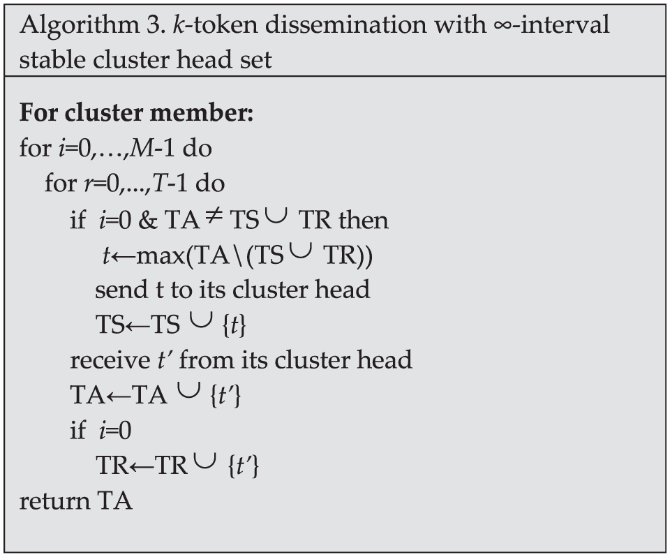
The algorithm for ∞-interval stable cluster head set.

The correctness of Algorithm 3 is proved as below.

Theorem 5

If the network has (k + α * L)-interval L-hop cluster head connectivity (Definition 7), each node will contain k tokens after executing n_h/α + 1 phases, where n_h is the number of cluster head nodes and α is a coefficient (it can be any positive integer).

Proof

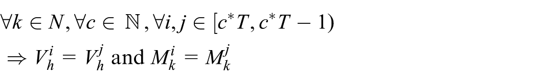
The proof is similar to that of Theorem 1. For a token t collected by any cluster member node u in the beginning of the first phase, there exists at least one cluster head that knows t in the end of the first phase. For any token t known by some cluster head v at the beginning of the phase i, there exists at least α cluster head nodes that newly learn token t in the end of phase i. Therefore, each the cluster head node contains k tokens after executing n_h/α phases. Then, in the next phase, they will broadcast the tokens in the same order. No matter how the node moves, all the nodes receive the same token in the same round in that phase. Then, each node will contain k tokens after executing n_h/α+1 phases. The theorem holds.

The modification to Algorithm 2 for the scenario of ∞-interval stable cluster head set is similar to the modification to Algorithm 1, as shown in Algorithm 3. The cluster member nodes only need to send all tokens in their TA sets in the first phase. The correctness of such modification can be proved as below.

Theorem 6

If the network has (α * L)-interval cluster head connectivity (Definition 5), each node will contain k tokens after executing M ≥ n_h/α + 1 rounds, where n_h is the number of cluster head nodes and α is a coefficient (it can be any positive integer).

Proof

For a token t collected by any cluster member node u in the beginning of the first round, at least one cluster head knows t in the end of the first round. Since the network has (α * L)-interval cluster head connectivity for any token t known by cluster head c in the round i, there are at least α cluster heads that newly learn t in the end of the round i + α * L. Therefore, each cluster head node contains k tokens after executing n_h/α round. Then, in the next round, they will broadcast the set of k tokens. No matter how nodes move, all of them will receive k tokens in that round. Then, each node will contain k tokens after executing n_h/α + 1 rounds. The theorem holds.

Theorem 7

If the network has L-interval stable hierarchy (Definition 4), each node will contain k tokens after executing M ≥ n_h * L + 1 rounds, where n_h is the number of cluster head nodes and α is a coefficient (it can be any positive integer).

Proof

The proof is similar to that of Theorem 6.

From one-hop clustering to multi-hop clustering

In the (T, L)-HiNet model, we consider only one-hop clustering, that is, all cluster members connect to the cluster head directly. Although such clustering is much more popular and practical than multi-hop clustering,³⁶ the latter is more general in terms of the capacity of clustering nodes. Therefore, we extend (T, L)-HiNet to (T, L, D)-HiNet to handle multi-hop clustering, where the distance between a cluster head and its members may be multiple hops.

Definition 9

(T-interval D-hop stable hierarchy): We say the cluster-based hierarchy is T-interval D-hop stable, such that $\forall k \in N, \forall c \in N, \forall i, j \in [c^{*} T, c^{*} T - 1) \Rightarrow V_{h}^{i} = V_{h}^{j} and M_{k}^{i} = M_{k}^{j}$ and there is a T-interval connectivity subgraph with distance(u, v) ≤ D in each cluster, where u is the cluster head and v is any cluster member. Then, based on T-interval D-hop stable hierarchy, we can extend (T, L)-HiNet from one-hop to multi-hop clusters.

Definition 10

(T, L, D)-HiNet: a dynamic network with T-interval D-hop stable hierarchy (Definition 9), and T-interval L-hop cluster head connectivity (Definition 7) is called (T, L, D)-HiNet.

Obviously, (T, L)-HiNet is the special case of (T, L, D)-HiNet with D = 1. To disseminate k tokens in (T, L, D)-HiNet, we need to modify Algorithm 1, as shown in Figure 7. The cluster head and gateway act the same as in Algorithm 1. The operations of cluster member nodes are different. A cluster member needs to send all tokens in its TA in three cases: in the first phase, upon affiliating a new cluster, and upon getting a new neighbor node in the same cluster. In other cases, the cluster member node sends all tokens in TN rather than TA. An example scenario of Algorithm 4 is shown in Figure 8. The correctness of the algorithm is proved as below.

Figure 7.

The algorithm for multi-hop clustering.

Figure 8.

An example illustration of Algorithm 4.

Theorem 8

If T ≥ k + α * L + D, each node will contain k tokens after executing M ≥ θ/α + 1 phases in Algorithm 4, where θ is the upper bound number of nodes that can be cluster head, and α is a coefficient (it can be any positive integer).

Proof

For a token t collected by any cluster member node u at the beginning of phase i, all nodes in $N_{i}^{T - k} (u)$ will get to known token t at the end of phase i. In a (T, L, D)-HiNet, the distance between u and its cluster head is at most D hops, so at least α cluster head nodes newly learn token t in the end of phase i. Since there are at most θ cluster heads, after θ/α phases, all the cluster head nodes should have collected all the k tokens. Because the cluster-based hierarchy is T-interval D-hop stable hierarchy (Definition 9), any token t known by some cluster head at the beginning of any phase i will be delivered to all nodes in the same cluster at the end of phase i. Then, after θ/α + 1 phases, all nodes must have collected the k tokens. The theorem holds.

Performance comparison and analysis

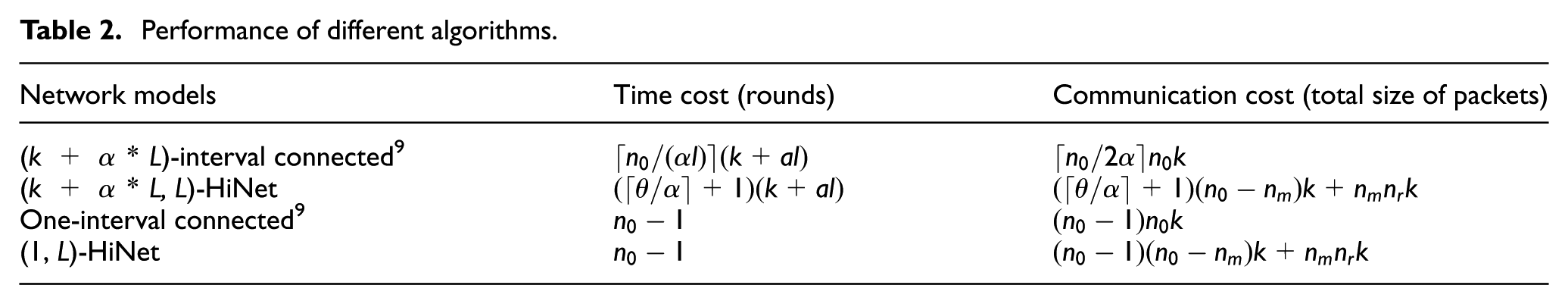
In this section, we analyze the performance of the proposed algorithms in terms of time cost and communication cost and compare them with the algorithms proposed in Kuhn et al.⁹ We choose⁹ because it is also based on the dynamic model of T-interval. We consider the two scenarios of dynamics adopted in section “Hierarchical information dissemination algorithms,” respectively, that is, (k + α * L, L)-HiNet and (1, L)-HiNet.

The number of nodes in the network is n₀. The upper bound number of nodes that can be cluster head is θ. The average number of cluster member nodes in one round is n_m. The re-affiliation count is incremented when a node gets dissociated from its cluster and becomes a member of another cluster. The average number of re-affiliations is n_r. In our analysis, time cost is represented by the number of rounds, and communication cost is represented by the total number of tokens sent. The time cost of each algorithm has been calculated in the correctness proof.

The communication cost is calculated as follows. In the algorithm in Kuhn et al.⁹ with (k + α * L)-interval connectivity, each node needs to broadcast in each phase. Since there are totally k tokens, each node broadcasts at most k times in one phase. Then, we can get the overall communication cost $⌈ n_{0} / 2 α ⌉ n_{0} k$ . In our algorithms, a cluster head/gateway node needs to broadcast in each phase, but a cluster member node broadcasts only when it re-affiliates to a new cluster head. Our communication cost is $(⌈ θ / α ⌉ + 1) (n_{0} - n_{m}) k + n_{m} n_{r} k$ . The analysis under one-interval connected model is similar (Table 1).

Table 1.

Notations used in performance analysis.

Notations	Descriptions
n ₀	The total number of nodes in the network
θ	The upper bound number of nodes that can be cluster head
n_m	The average number of cluster member nodes in one round
n_r	The average number of re-affiliations a cluster member conducts
k	The number of tokens to be disseminated
α	A coefficient. It can be any positive integer

Table 2 shows the results of both time cost and communication cost under different dynamics models. The communication cost of our algorithm in (1, L)-HiNet is $(n_{0} - 1) (n_{0} - n_{m}) k + n_{r} n_{m} k$ , while the communication cost in Kuhn et al.⁹ is $(n_{0} - 1) (n_{0} - n_{m}) k + (n_{0} - 1) n_{m} k$ . Since n_r should be much less than n₀, the communication cost of our algorithm is much less than that of Kuhn et al.⁹ This is obviously the benefit of hierarchical design.

Table 2.

Performance of different algorithms.

Network models	Time cost (rounds)	Communication cost (total size of packets)
(k + α L*)-interval connected⁹	$⌈ n_{0} / (α l) ⌉ (k + al)$	$⌈ n_{0} / 2 α ⌉ n_{0} k$
(k + α L, L*)-HiNet	$(⌈ θ / α ⌉ + 1) (k + al)$	$(⌈ θ / α ⌉ + 1) (n_{0} - n_{m}) k + n_{m} n_{r} k$
One-interval connected⁹	$n_{0} - 1$	$(n_{0} - 1) n_{0} k$
(1, L)-HiNet	$n_{0} - 1$	$(n_{0} - 1) (n_{0} - n_{m}) k + n_{m} n_{r} k$

To show the advantage of our design more clearly, we calculate information dissemination costs with an example network setup (in Table 3). The number of nodes in the network is 100. The upper bound number of nodes that can be cluster head is 30. The average number of cluster members in one round is 40. The average number of re-affiliations is set to be 3 and 10 in (T, L)-HiNet and (1, L)-HiNet, respectively. This is because in a (1, L)-HiNet, the dynamics is higher and consequently, re-affiliations should occur more times. The number of tokens is set to be eight. The values of α and L are set to be 5 and 2, respectively.

Table 3.

Numerical results of performance analysis.

Models of dynamic networks	Spending time (rounds)	Communication cost (total size of packets)
(k + α L*)-interval connected⁹	180	8000
(k + α L, L*)-HiNet	126	4320
One-interval connected⁹	99	79,200
(1, L)-HiNet	99	51,680

As shown in Table 3, the communication cost of our algorithms is much less than that algorithms in Kuhn et al.⁹ At the same time, the time cost of our algorithms is the same as or even smaller than that of the algorithms in Kuhn et al.⁹ Although these are just results from one example setting, they still validate the advantage of our design to some extent.

Now we analyze the communication cost of clustering algorithms. The most existing clustering algorithms consist of two phases: cluster formation and cluster maintenance. In cluster formation phase, each node exchanges messages to share neighborhood information. The communication cost in such phase is about 3 * n₀. In cluster maintenance phase, the node requires to exchange messages when a cluster member node re-affiliates to a new cluster or a cluster member/gateway node becomes a new cluster head. The communication cost of the re-affiliation and the re-clustering is about 3 * n_rn_m and 3 * n_c, respectively, where n_c is the number of the nodes that participate in re-clustering a new cluster. Thus, the communication cost of clustering algorithm is about 3 * (n₀ + n_rn_m + n_c). In a good cluster algorithm, n_c should be less than n₀; the communication cost of clustering algorithm is much less than that of the k-token dissemination algorithm.

Simulation results

To validate the correctness of our algorithms and measure their performance quantitatively, we simulate the proposed algorithms using ns3. Kuhn et al.⁹ and Haeupler and Karger¹⁰ are the latest papers that study k-token dissemination problem. Haeupler and Karger¹⁰ used network coding for token dissemination, which is not considered in our paper. Thus, we simulated the token dissemination algorithm proposed in Kuhn et al.⁹ for comparison purpose. Note that the simulation is to validate the correctness of our algorithms rather than engineering experiment; the simulation environment is based on the assumption of our model.

We simulate a network with totally N nodes and they are distributed in a 2000 m × 2000 m area randomly. IEEE 802.11b protocol is used for wireless communication, with a radio range of 300 m. The maximum node speed is 100m per round. In the beginning, there are k tokens, owned by k nodes.

To clustering the nodes, we simulate the highest degree algorithm,³⁶ where the node with the highest degree of connectivity among neighbors is selected as a cluster head. Corresponding to our (T, L)-HiNet model, we set L = 2 in the clustering.

The performances of token dissemination algorithms are measured using two metrics for time cost and communication cost, respectively. The time cost is defined as the number of rounds used for all the nodes to collect all the k tokens. The communication cost is measured by the total number of broadcasting conducted by all the nodes.

In the simulations, we vary the values of major parameters, including T, N, and k to examine different cases. The number of nodes is varied from 100 to 200. The other two parameters are set with respect to N. The value of M is equal to $⌈ t / T ⌉$ , where t is the number of rounds used for all the nodes to collect all the k tokens. Since T is a key parameter for our algorithm, we first examine its effect and then compare our algorithm with the one proposed in Kuhn et al.⁹

The effect of T

In this part, we examine the effect of T on the performance of our algorithm. As aforementioned, to successfully disseminate k tokens, T must be not less than k. For simulating more different values of T, we consider the scenarios with few tokens, that is, k = 4. With k = 4, we simulate our algorithm under T from 4 to 25. T = 4 stands for the scenarios with minimum requirement, while T = 25 means ∞-interval connectivity in the scenarios. The number of nodes is set to 120 and 160. From Figures 9 and 10, we can see that with the increase of T, both the time cost and communication cost decrease first and then keep being stable. This indicates that high stability can help reducing information dissemination cost, but the reduction becomes very minor when the network is stable enough. For the simulated cases with k = 4, such situation occurs in the range of 5–10.

Figure 9.

Time cost against T, with k = 4.

Figure 10.

Communication cost against T, with k = 4.

Comparison with the algorithm in Kuhn et al.

In this part, we simulate more cases and compare our algorithm with the one in Kuhn et al.⁹ to show the benefit of our design. According to the value of k, our simulation can be divided into two parts: k = 4 and k = N. The former stands for the scenarios with few tokens and initiators, while the latter stands for the scenarios with a large number of tokens and initiators, that is, all-to-all dissemination.

Results with k = 4

The value of N is varied between 100 and 200 to show the effect of node number. The results with T = k = 4 are shown in Figures 11 and 12.

Figure 11.

Time cost comparison with T = k = 4.

Figure 12.

Communication cost comparison with T = k = 4.

Figure 11 shows the time cost of different algorithms under varied node numbers. It is interesting to see that the time cost decreases with the increase of number of nodes. This can be explained as follows. With a fixed area, the increase of nodes will result in the increase of node density. Consequently, the average distance between nodes may be decreased. Since all dissemination operate based on hop-by-hop broadcasting, higher node density will reduce the total time to deliver the tokens.

Now, let us compare the two algorithms. The results in Figure 11 show that our algorithm can deliver all tokens within fewer rounds. This is an interesting difference. The reduction is about 20% under various numbers of nodes. Intuitively, the algorithm in Kuhn et al.⁹ should deliver tokens faster than ours because that algorithm let all nodes keep broadcasting. We believe that the reduction of time cost of our algorithm should come from the reduction of transmission collisions. All the nodes broadcast token messages in each round in Kuhn et al.,⁹ while in our algorithm only part of nodes broadcast token messages in each round. Obviously, fewer transmissions are done by our algorithm and consequently fewer collisions may occur. More collisions will cause more waiting and re-try and certainly result in more rounds to deliver tokens.

The effect of node number on communication cost is quite different from that on time cost. As shown in Figure 12, the communication cost increases with the increase number of nodes. Compared with the algorithm in Kuhn et al.,⁹ our algorithm can save obviously communication, and reduction is roughly 40% under various numbers of nodes. This definitely indicates the benefit of hierarchical design.

The results with k = 4 and T = 6 are shown in Figures 13 and 14. Same as the results with T = 4, communication cost of both algorithms increases with the increase of node number, and our algorithm can significantly reduce both communication cost and time cost. This indicates that our algorithm can outperform the algorithm in Kuhn et al.⁹ with different T values.

Figure 13.

Time cost comparison with T = 6 and k = 4.

Figure 14.

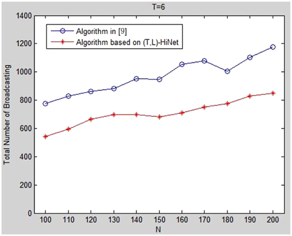
Communication cost comparison with T = 6 and k = 4.

Results with k = N

In this part, we focus on the all-to-all dissemination scenarios. Since the value of T must not be less than k, we set T = N in this part of simulations.

Figure 15 shows the time cost of all-to-all dissemination under various N. With the increase of N, the time cost of both the algorithms changes but not increases or decreases obviously. This can be explained by the combination of the effect of node density and the effect of number of tokens. On one hand, a larger N results in a larger node density and consequently a smaller time cost, which has been discussed in the scenarios of k = 4. On the other hand, more tokens will trivially cost more rounds to disseminate. Combining the two effects, the time cost with k = N roughly keeps in the same level when N increases. Different from time cost, the communication cost of both algorithms increases with the increase of N, as shown in Figure 16. This is straightforward. More tokens will certainly introduce more broadcasting at each node and more nodes will certainly increase the total number of broadcasting operations.

Figure 15.

Time cost comparison with T = k = N.

Figure 16.

Communication cost comparison with T = k = N.

Comparing with the algorithm in Kuhn et al.,⁹ our algorithm can always reduce time cost and communication cost under various cases of N. The average reduction of time cost is about 25%, while the average reduction of communication is roughly 45%. This further confirms the benefit of hierarchical design.

Conclusion and future work

We study information dissemination in dynamic networks, with the consideration of cluster-based hierarchy to reduce communication cost. Our work includes model definition, algorithm design, correctness proof and performance analysis. Based on the notion of T-interval connectivity proposed by Kuhn et al.,⁹ we define a new dynamic network model, named (T, L)-HiNet, which defines the stability of cluster-based hierarchy on top of dynamic topology. Based on (T, L)-HiNet, we design hierarchical information dissemination algorithms for different dynamics scenarios. We also extend the (T, L)-HiNet model in two different directions: from T-interval to ∞-interval stable cluster head, and from one-hop clustering to multi-hop clustering. With the help of clusters, information from cluster members is disseminated along connections among cluster head, and consequently, fewer packets need to be transmitted. Performance evaluations via both analysis and simulation show that compared with the algorithms designed in Kuhn et al.,⁹ our solution can disseminate information with much less communications cost while the time cost is similar or even smaller, and the benefit can be as much as 50%.

Much more efforts are needed to extend and improve the work that considers clusters in dynamic networks. One interesting direction is to extend other flat dynamic network models, for example, dynamic diameter, EMDG, should also be extended with clusters.

Footnotes

Acknowledgements

This article is an extension of our conference paper published in the proceedings of ICPP’13³⁷ (the 42th International Conference on Parallel Processing). In the extend version, we have added quite a lot of new and significant content to make our work more solid and significant. We have added new algorithms under more network models, which make our work more general. We have conducted simulations to examine the performance of our algorithms and compare them with existing ones, which make confirm our objective of algorithm design with quantitatively.

More precisely, we list the difference between this article and the conference version as follows:

1. We have added algorithms for ∞-interval stable cluster head set (section “From T-interval stable cluster head set to ∞-interval stable cluster head set”).

The case of ∞-interval stability is a special case of the T-interval stability. In the conference version, we simply discussed the case of ∞-interval stable cluster head set in (T, L)-HiNet, without algorithms presented.

In the journal version, we provide detailed design of the new algorithms by extending the one for T-interval stability. With ∞-interval stable cluster head set, communication cost can be further reduced. The new algorithms are also proved to be correct.

2. We have added algorithms for the cases of multi-hop clusters (section “From one-hop clustering to multi-hop clustering”).

In the conference version, we assume one-hop clusters. Multi-hop clustering is the generalization of one-hop clusters. In the journal version, we extend our (T, L)-HiNet model to a more general model of (T, L, D)-HiNet. Based on the new model, we present modifications to our one-hop algorithms for multi-hop clusters and also prove the correctness.

3. We have added the simulations via ns3 to evaluate the performance of our algorithms and compare them with existing ones. Our work is motivated by reducing communication cost in token dissemination, which is a concern on performance. Simulations confirm the benefit of our design very well, which makes our work more solid and convincing.

4. We have added the discussion on handling node failures. This makes our work more complete in terms of fault tolerance.

Handling Editor: Alessandro Bogliolo

Declaration of conflicting interests

The author(s) declared no potential conflicts of interest with respect to the research, authorship, and/or publication of this article.

Funding

The author(s) disclosed receipt of the following financial support for the research, authorship, and/or publication of this article: This research is partially supported by National Key Research and Development Program of China (2016YFB0200404), National Natural Science Foundation of China (nos U1711263, 61379157, and 61472455), Program of Science and Technology of Guangdong (no. 2015B010111001), Guangzhou Science and Technology Bureau (201704020030), and MOE-CMCC Joint Research Fund of China (no. MCM20160104).

References

Kempe

Kleinberg

Kumar

. Connectivity and inference problems for temporal networks. In: Proceedings of the 32nd annual symposium on theory of computing, Portland, OR, 21–23 May 2000, pp.504–513. New York: ACM.

Grindrod

Higham

DJ.

Evolving graphs: dynamical models, inverse problems and propagation. P R Soc A 2010; 466(2115): 753–770.

Kuhn

Oshman

Dynamic networks: models and algorithms. ACM SIGACT News 2011; 42: 82–96.

Leskovec

Kleinberg

Faloutsos

Graph evolution: densification and shrinking diameters. ACM T Knowl Discov D 2007; 1: 1–41.

Datta

Giannella

Kargupta

K-means clustering over a large, dynamic network. In: Proceedings of the 6th international conference on data mining, Bethesda, MD, 20–22 April 2006, pp.153–164. Philadelphia, PA: SIAM.

Krishna

Vaidya

Chatterjee

et al . A cluster-based approach for routing in dynamic networks. ACM SIGCOMM Comp Com 1997; 27(2): 49–64.

Hromkovĭc

Klasing Monien

et al . Dissemination of information in interconnection networks (broadcasting & gossiping). Comb Netw Theory 1996; 1: 125–212.

O’Dell

Wattenhofer

Information dissemination in highly dynamic graphs. In: Proceedings of the 9th joint workshop on foundations of mobile computing, Cologne, 2 September 2005, pp.104–110. New York: ACM.

Kuhn

Lynch

Oshman

Distributed computation in dynamic networks. In: Proceedings of the 42nd symposium on theory of computing, Cambridge, MA, 5–8 June 2010, pp.513–522. New York: ACM.

10.

Haeupler

Karger

Faster information dissemination in dynamic networks via network coding. In: Proceedings of the 30th annual symposium on principles of distributed computing, San Jose, CA, 6–8 June 2011, pp.381–390. New York: ACM.

11.

Hedetniemi

Liestman

A survey of gossiping and broadcasting in communication networks. Networks 1988; 18: 319–349.

12.

Baumann

Crescenzi

Fraigniaud

Parsimonious flooding in dynamic graphs. In: Proceedings of the 28th symposium on principles of distributed computing, Calgary, AB, 10–12 August 2009, pp.260–269. New York: ACM.

13.

Topkis

DM.

Concurrent broadcast for information dissemination. IEEE T Software Eng 1985; SE-11(10): 1107–1112.

14.

Cao

Raynal

Eventual clusterer: a modular approach to designing hierarchical consensus protocols in MANETs. IEEE T Parall Distr 2009; 20(6): 753–765.

15.

Cao

Yang

et al . Design and performance evaluation of efficient consensus protocols for mobile ad hoc networks. IEEE T Comput 2007; 56(8): 1055–1070.

16.

Friedman

Kogan

Deterministic dominating set construction in networks with bounded degree. Lect Notes Comput Sc 2011; 6522: 65–76.

17.

Wang

Nodes neighborhood relation-based constructing algorithm for minimum connected dominating set. Comput Eng 2010; 36(13): 105–107.

18.

Mao

Anderson

BDO

. On the properties of one-dimensional infrastructure-based wireless multi-hop networks. IEEE T Wirel Commun 2012; 11(7): 2606–2615.

19.

Cardei

Dai

et al . Extended dominating set and its applications in ad hoc networks using cooperative communication. IEEE T Parall Distr 2006; 17(8): 851–864.

20.

Clementi

Macci

Monti

et al . Flooding time in edge-Markovian dynamic graphs. In: Proceedings of the 27th symposium on principles of distributed computing, Toronto, ON, 18–21 August 2008, pp.213–222. New York: ACM.

21.

Akrida

Gasieniec

Mertzios

et al . Ephemeral networks with random availability of links: diameter and connectivity. In: Proceedings of the 26th symposium on parallelism in algorithms and architectures, Prague, 23–25 June 2014, pp.267–276. New York: ACM.

22.

Avin

Kouck’y

Lotker

. How to explore a fast-changing world (cover time of a simple random walk on evolving graphs). In: Proceedings of the 35th international colloquium on automata, languages and programming, Reykjavik, 7–11 July 2008, pp.121–132. New York: ACM.

23.

Yang

Chen

et al . Accurate and efficient counting in dynamic networks. In: Proceedings of the 33rd international symposium on reliable distributed systems, Nara, Japan, 6–9 October 2014, pp.301–310. New York: IEEE.

24.

Ducourthial

Wade

. Dynamic p-graphs for capturing the dynamics of distributed systems. Ad Hoc Netw 2016; 50: 13–22.

25.

Casteigts

Flocchini

Quattrociocchi

et al . Time-varying graphs and dynamic networks. Int J Parallel Emerg Distrib Syst 2012; 27: 387–408.

26.

Wehmuth

Fleury

Ziviani

. A unifying model for representing time-varying graphs. Research report, Report no. 8466, January2014. Rocquencourt: Inria.

27.

Mosk-Aoyama

Shah

Computing separable functions via gossip. In: Proceedings of the 25th annual symposium on principles of distributed computing, Denver, CO, 23–26 July 2006, pp.113–122. New York: ACM.

28.

Kempe

Dobra

Gehrke

. Gossip-based computation of aggregate information. In: Proceedings of the 44th annual symposium on foundations of computer science, Cambridge, MA, 11–14 October 2003, pp.482–491. New York: IEEE.

29.

Pittel

On spreading a rumor. SIAM J Appl Math 1987; 47(1): 213–223.

30.

Jelasity

Guerraoui

Kermarrec

et al . The peer sampling service: experimental evaluation of unstructured gossip-based implementations. In: Proceedings of the 5th ACM/IFIP/USENIX international conference on middleware, Toronto, ON, 18–22 October 2004, pp.79–98. New York: Springer-Verlag.

31.

Clementi

Monti

Silvestri

Flooding over Manhattan. In: Proceedings of 29th symposium on principles of distributed computing, Zurich, 25–28 July 2010, pp.375–383. New York: ACM.

32.

Pettarin

Pietracaprina

Pucci

et al . Tight bounds on information dissemination in sparse mobile networks. In: Proceedings of the 30th symposium on principles of distributed computing, San Jose, CA, 6–8 June 2011, pp.355–362. New York: ACM.

33.

Sarma

Molla

Pandurangan

Distributed computation in dynamic networks via random walks. Theor Comput Sci 2015, 581: 45–66.

34.

Augustine

Chen

Liaee

et al . Information spreading in dynamic networks under oblivious adversaries. In: Gavoille

Ilcinkas

(eds) Distributed computing. Berlin: Springer, 2016, pp.399–413.

35.

Michail

Chatzigiannakis

Spirakis

PG.

Causality, influence, and computation in possibly disconnected synchronous dynamic networks. J Parallel Distr Com 2014; 74(1): 2016–2026.

36.

Chong

PHJ

. A survey of clustering schemes for mobile ad hoc networks. IEEE Commun Surv Tut 2005; 7(1): 32–48.

37.

Yang

Chen

et al . Efficient information dissemination in dynamic networks. In: Proceedings of the 42nd international conference on parallel processing, Lyon, 1–4 October 2013, pp.593–602. New York: IEEE.

Cluster-based efficient information dissemination in dynamic networks

Abstract

Keywords

Introduction

Related work

(T, L)-HiNet: a hierarchical dynamic network model

System model

Definition of CTVG

Definition 1

Definition of (T, L)-HiNet

Definition 2

Definition 3

Definition 4

Definition 5

Definition 6

Definition 7

Definition 8

Hierarchical information dissemination algorithms

The algorithm for (T, L)-HiNet

Description of algorithm operations

Correctness proof

Lemma 1

Proof

Lemma 2

Proof

Theorem 1

Proof

Handling node failures

The algorithm for (1, L)-HiNet

Theorem 2

Proof

Theorem 3

Proof

Theorem 4

Proof

Extensions to (T, L)-HiNet

From T-interval stable cluster head set to ∞-interval stable cluster head set

Theorem 5

Proof

Theorem 6

Proof

Theorem 7

Proof

From one-hop clustering to multi-hop clustering

Definition 9

Definition 10

Theorem 8

Proof

Performance comparison and analysis

Simulation results

The effect of T

Comparison with the algorithm in Kuhn et al.

Conclusion and future work

Footnotes

Acknowledgements

Declaration of conflicting interests

Funding

References