Sage Journals: Discover world-class research

Abstract

In ubiquitous streaming data sources, such as sensor networks, clustering nodes by the data they produce gives insights on the phenomenon being monitored. However, centralized algorithms force communication and storage requirements to grow unbounded. This article presents L2GClust, an algorithm to compute local clusterings at each node as an approximation of the global clustering. L2GClust performs local clustering of the sources based on the moving average of each node’s data over time: the moving average is approximated using memory-less statistics; clustering is based on the furthest-point algorithm applied to the centroids computed by the node’s direct neighbors. Evaluation is performed both on synthetic and real sensor data, using a state-of-the-art sensor network simulator and measuring sensitivity to network size, number of clusters, cluster overlapping, and communication incompleteness. A high level of agreement was found between local and global clusterings, with special emphasis on separability agreement, while an overall robustness to incomplete communications emerged. Communication reduction was also theoretically shown, with communication ratios empirically evaluated for large networks. L2GClust is able to keep a good approximation of the global clustering, using less communication than a centralized alternative, supporting the recommendation to use local algorithms for distributed clustering of streaming data sources.

Keywords

Distributed clustering data streams local algorithms

Introduction

Nowadays, information is generated and gathered from distributed data sources, at a very high rate, stressing communications and computing infrastructure. Basically, data are being produced continuously everywhere. To make sense of these ubiquitous data streams, knowledge discovery techniques, which try to extract patterns and concepts from raw data, have become a major tool for all sorts of applications. One of the most popular knowledge discovery techniques is clustering, the process of finding groups in data such that data objects clustered in the same group are more alike than objects assigned to different groups.

Clustering streaming data sources is the task of clustering different sources of data streams, based on the data series similarity.¹ Algorithms aim to find groups of data sources that behave similarly through time, which is usually measured in terms of the distance between the data series or the data distribution. The goal of an incremental clustering system for streaming data sources is to find (and make available at any time t) a partition P of those sources, where data sources in the same cluster tend to be more alike than data sources in different clusters.² But classical methods tend to become obsolete for application in streaming and (especially) ubiquitous settings, due to their high time and space complexity. Hence, new machine learning algorithms are being developed to cope with this new demanding scenario, and different quality indices and evaluation strategies are being considered.³

The aim of our work is to enable the clustering of distributed streaming data sources without a centralized control process, building on the following research question: can local algorithms approximate the global clustering of the entire network without a centralized server? Specifically, we intend to define a general approach to achieve a global clustering definition locally at each node, without a central server and validate whether quality clustering can be achieved with such procedure. The test setting of our study is sensor networks, given their distributed and resource-demanding characteristics. Moreover, in this article, we will focus on sensors producing univariate streams of data, performing clustering based on the moving average of each sensor’s data, but restraining communication to direct neighbors in order to avoid message forwarding, thus improving energy savings. We should stress that our problem is not to cluster sensor nodes for transmission purposes in wireless sensor networks,⁴ rather find groups of sensors that generate similar data.

The aim of the evaluation is to assess quality in terms of agreement between local clustering definitions and the global clustering definition. Also evaluated is the communication reduction and robustness to communication incompleteness.

Rationale

Data are often ubiquitously produced. For example, data are generated by web clicks or network package routing on each machine; global positioning system (GPS) devices produce and process data locally; peer-to-peer applications even disregard centralized server processing; cellphone applications produce data from phone calls, text messaging, and wireless connections; and deep sky data are now being generated by telescope ensembles. The amount of data being produced in information and industrial systems is so high that no single database can hold all information. Rather, these data are produced, possibly stored, and definitely should be processed in distributed locations.

Paradigmatic examples of distributed streaming data sources are sensor networks and health information systems. Also, mobile computing devices like personal digital assistants (PDAs), cell phones, wearables, and smart cards play an increasingly important role in our daily life. The emergence of powerful mobile devices with reasonable computing and storage capacity is ushering an era of advanced data and computationally intensive mobile applications.⁵ Our world is evolving into a setting where all devices, as small as they may be, will be able to include sensing and processing ability.⁶ However, different types of devices present different levels of resources, and care should be taken in data mining methods that aim to extract knowledge from such restricted scenarios.⁷ Given their ubiquitous characteristic (spatially distributed and continuous monitoring) and resource management requirements (e.g. battery), in the remainder of this article, we will focus on sensor network scenarios as an example of ubiquitous data sources.

Clustering data-stream sources

Clustering is probably the most frequently used data mining algorithm, used as exploratory data analysis.⁸ The main problem in applying clustering to data streams is that systems should consider data evolution, being able to compress old information and adapt to new concepts. Two different clustering problems exist: clustering streaming data points and clustering streaming data sources. Clustering streaming data points is the task of clustering data flowing from a continuous stream, based on data points similarity,⁹ aiming to discover structures in data over time.¹⁰ Algorithms usually search for dense regions of the data space, identifying hot-spots where streaming data sources tend to produce data.⁶ Clustering streaming data sources is the task of clustering different sources of data streams based on the data series similarity.¹¹ Algorithms aim to find groups of data sources that behave similarly through time, which is usually measured in terms of the distance between the data series or the data distribution. The goal of an incremental clustering system for streaming data sources is to find (and make available at any time t) a partition P of those sources, where data sources in the same cluster tend to be more alike than data sources in different clusters.²

Distributed clustering of streaming sources

Several issues emerge in the development of new techniques to efficiently and effectively perform clustering of distributed streaming data sources.¹ This is an emerging area of research which has been already studied in various fields of real-world applications.^11–13 However, algorithms previously proposed tend to deal with data as a centralized multivariate stream.⁶ They are designed as a single process of analysis, without taking into account the locality of data produced by sources on a distributed scenario, the transmission and processing resources of the network, and the breach in the transmitted data quality.

Most works on clustering analysis for distributed sources (e.g. sensor networks) actually concentrate on clustering the sources by their geographical position^14,15 and connectivity, mainly for power management¹⁶ and network routing purposes.¹⁷ However, in this topic, we are interested in clustering techniques using the data produced by the sources, instead.

In previous work,¹⁸ the requirements of clustering distributed streaming data sources have been discussed and enumerated: (a) the requirements for clustering streaming data sources must be considered, with more emphasis on the adaptability of the whole system; (b) processing must be distributed and synchronized on local neighborhoods or querying nodes; (c) the main focus should be on finding similar data sources irrespective to their physical location; (d) processes should minimize different resources (mainly energy) consumption in order to achieve high uptime; and (e) operation should consider a compact representation of both the data and the generated models, enabling fast and efficient transmission and access from mobile and embedded devices.

Many algorithms have been developed for distributed clustering in peer-to-peer environments and sensor networks settings. However, they do not target our problem, as they might operate with a central server,^19,20 are directed toward data clustering and not data sources,^21,22 address homogeneous distributed clustering—each node having a sample of the same data^23,24—or, if they target clustering of streaming data sources, they take into account the network infrastructure in the process of finding a clustering definition.²⁵ The final goal is to infer a global clustering structure of all relevant data sources. Hence, approximate algorithms should be considered to prevent global data transmission.

Advantages of application

Although transversely relevant to most ubiquitous applications, the advantages of distributed clustering of streaming data sources are better analyzed in specific real-world applications.

On real-world domains

In electricity supply systems, the identification of demand profiles (e.g. industrial or urban) by clustering streaming sensors’ data decreases the computational cost of predicting each individual subnetwork load.²⁶ This is a common scenario with thousands of different sensors distributed over a wide area. As sensors are naturally distributed in the electrical network, distributed procedures which would focus on local networks could prevent the dimensionality drawback.

A common problem in geoscience research is the monitoring of natural phenomena evolution. Several techniques are currently being used to address these problems, and given their increasing availability, sensor-based approaches are now hot topics in the area. Sensor nodes can be densely deployed either very close or directly inside the phenomenon to be observed:²⁷ ocean streams or river flows, a twister or a hurricane, and so on. Sensors deployed in the objective area can monitor several measures of interest, such as water temperature, stream gauge, and electricity resistance. Clustering the data produced by different sensors is helpful to identify areas with similar profiles, possibly indicating actual water or wind streams.

The GPS is commonly used to monitor location, speed, and direction of both people and objects. Identifying similar paths, for example, in delivery teams or traffic flow, is a relevant task to current enterprises and end users.²⁸ Embedding these systems with context information is now a major research challenge to be able to improve results with real-time information.²⁹ However, the amount of data produced by each GPS receiver is so huge, and the allowed latency so narrow, that performing centralized clustering of GPS tracks becomes too expensive. If each receiver is used to perform a distributed procedure for the clustering task, the same goal should be achieved faster with better resource management.

In medical environments, clustering medical sensor data (such as electrocardiogram (ECG) and electroencephalogram (EEG)) is useful to determine association between signals,³⁰ allowing better diagnosis. Detecting similar profiles in these measures among different patients is one way to explore uncommon conditions. Mobile and embedded devices could interconnect different patients and physicians, without revealing sensible information from patients while nevertheless achieving the goal of identifying similar profiles.

On sensor network management

Distributed clustering of streaming data sources presents advantages for everyday processing in sensor networks. We can point out the implications in three areas: message forwarding, deployment quality, and privacy preservation.

One of the highest resources consuming tasks in sensor networks is communication. Moreover, information is usually forwarded through the network into a sink node. With sensors increasing in number, redundant information is also more probable, so message forwarding will become a heavy-resource leak. If a distributed clustering procedure is applied at each forwarding node, usual data aggregation techniques could be data-centric, in the sense that one node could decide not to transmit a message, or aggregate it with others, if it contains information which is quite similar to other nodes.

When sensor networks are deployed in objective areas, the design of this deployment is most of the times subject to expert-based analysis or template-based configuration. Unfortunately, the best deployment configuration is sometimes hard to find. Applying distributed clustering of sensors’ data streams, the system can identify sensors with similar reading profiles, while investigating whether the sensors are in the same geographical cluster. If similar sensors, with respect to the produced data, are placed in a dense, with respect to the geographical position, cluster of sensors, then resources are spoiled as some of the sensors would give the same information. These sensors could then be assigned to different positions in the network.

The privacy of personal data is most of the times important to preserve, even when the objective is to analyze and compare with other people’s data. Anonymization is the most common procedure to ensure this but experience has shown that it is not flawless. This way, centralizing all information in a common data server could represent a more vulnerable setup for security breaches. If we can achieve the same goal without centralizing the information, privacy should be easier to preserve. Furthermore, the system could achieve a global clustering structure without sharing sensible information between all nodes in the network, somewhat similar to clustering using the fractal dimension.³¹

On sensor network comprehension

Sensor network comprehension tries to extract information about global interaction between sensors by looking at the data they produce.⁶ However, common applications usually inspect behaviors of single sensors, looking for threshold-breaking values or failures. To increase the ability to understand the inner dynamics of the entire network, deeper knowledge should be extracted.

The distributed setup proposed in this section enables a transient user to query a local node for its position in the overall clustering structure of sensors, without asking the centralized server. For example, a query for a given sensor could be answered as “this sensor and sensors 2 and 3 are highly correlated” in the sense that when one’s values increase, the other sensors’ values also increase or “the answering sensor is included in a group of sensors that has the following profile or prototype of behavior.” Hence, the comprehension of how sensors are related in the network is also greatly improved by using distributed sensor clustering techniques.

Consider mobile sensor networks where each sensor produces a stream with its current GPS location. Clustering the examples would give an indication of usual dispersion patterns, while clustering the sensors could give indication of physical binding between sensors, forcing them to move with similar paths. Another application could rise from temperature/pressure sensors placed around geographical sites such as volcanoes or seismic faults. Furthermore, the evolution of these clustering definitions is also relevant. If each sensor’s stream consists of IDs of the sensors for which this sensor is forwarding messages, changes in the clustering structure would indicate changes in the physical topology of the network, as dynamic routing strategies are commonly encountered in current sensor network applications. Overall, the main goal of sensor network comprehension is to apply automatic unsupervised procedures to discover interactions between sensors, trying to exploit dynamism and robustness of the network being deployed.⁶

L2GClust—local-to-global clustering

A local algorithm is proposed to approximate the global clustering of sensors on ubiquitous sensor networks, based on the moving average of each node’s data over time. There are two main characteristics. On one hand, each sensor node keeps a sketch of its own data. On the other hand, communication is limited to direct neighbors, so clustering is computed at each node. The moving average of each node is approximated using memoryless fading average, while clustering is based on the furthest-point algorithm applied to the centroids computed by the node’s direct neighbors. This way, each sensor acts not only as data stream source but also as a processing node, keeping a sketch of its own data and a definition of the clustering structure of the entire network of data sources.

On one hand, local algorithms are one of the most efficient family of algorithms developed for distributed systems. Local algorithms are in-network algorithms in which data are never centralized, but rather, computation is performed by the peers of the network. In a local algorithm, it often happens that the resources needed to compute the function are independent of the size of the system, therefore exhibiting high scalability, in comparison with their global counterparts.³² On the other hand, averages can be viewed as the values minimizing quadratic cost functions. Quadratic optimization problems are very special since their solutions are linear functions of the data, in which case a simple accumulation process leads to a solution.³³ Hence, there is a relevance in monitoring average values.

In this work, we search for a definition of k clusters of sensor nodes, with k previously known by the system. Although this simple problem statement lacks some of the common characteristics of real-world scenarios (e.g. unknown number or clusters or unbalanced data), its extension is straightforward. Figure 1 presents a simple and illustrative toy example of the outcomes that such a local algorithm should achieve, using incremental average computations and incremental k-means clustering at each node.

Figure 1.

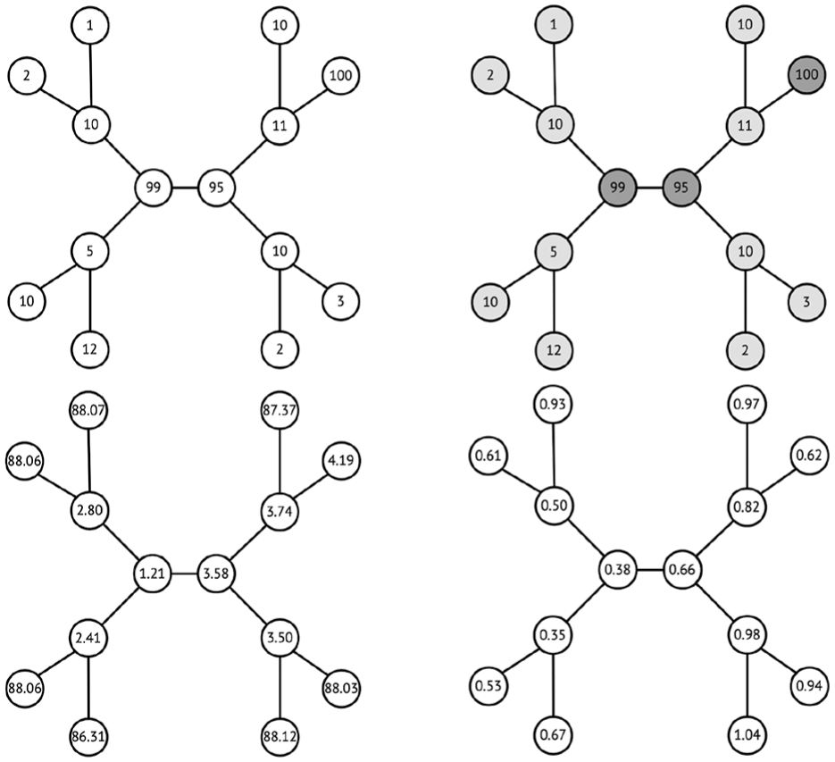
Toy example of a sensor network: in top plots, each sensor s produces a stream $X_{s} ~ N (μ_{s}, 0.5)$ , link connections are represented by edges, and vertex labels indicate each sensor’s concept $(μ_{s})$ . Top right plot presents a possible two-cluster partition of the conceptual means produced by the nodes. After initial three iterations (bottom left), each node has estimates of the global clusters centroids, but are rather biased toward local neighborhoods (numbers in the nodes represent the Euclidean distance between local estimates and real centroids ${6.9, 98.0}$ ). After 150 iterations of exchanging only the cluster centroids’ estimates (bottom right), all nodes have already good estimates of the global centroids. Most important to note is that although having slightly different estimates (not shown in the example), all nodes would correctly assign all nodes to the correct cluster.

Local data stream sketches

As previously stated, we consider that each sensor produces a univariate stream of data, and we want to define a clustering structure for the sensors, where sensors producing streams which are alike are clustered together. Hence, we should consider techniques that project each sensor’s data stream into a reduced set of dimensions which suffice to extract similarity with other sensors. These estimates can be seen as the sensor’s current view of its own data, giving a sign of where in the data space this sensor is included.⁶ One simple way to summarize a data stream x is by computing its sample mean ${\hat{μ}}_{x}$ and standard deviation ${\hat{σ}}_{x}$ . Our approach is to keep track of the moving average of each sensor, as an estimate of the sample mean of most recent data.

Memory-less fading average

Each sensor produces data continuously. Given this, each sensor s is responsible of keeping its own estimate of the sample mean $({\hat{μ}}_{s})$ in a online fashion. Moving averages are usually easy to compute, if we can keep a small buffer of data points.³⁴ However, in such resource-demanding scenarios, this is seldom the case. Nonetheless, sum-based statistics computed on sliding windows can be approximated by weighting the sums using fading statistics.³⁵ The $α$ -fading sum $S_{x, α} (i)$ of observations from a stream x is computed at time $\forall i > 0$ as

S_{x, α} (i) = x_{i} + α \times S_{x, α} (i - 1)

where $S_{x, α} (0) = 0$ . In the computation, $α$ $(0 << α < 1)$ is a constant determining the forgetting factor of the sum. This way, the $α$ -fading average at observation $\forall i > 0$ is then computed as

M_{x, α} (i) = \frac{S_{x, α} (i)}{N_{α} (i)}

where $N_{α} (i) = 1 + α \times N_{α} (i - 1)$ is the corresponding $α$ -fading increment, with $N_{α} (0) = 0$ . An important feature of the $α$ -fading increment is that

lim_{i \to + \infty} N_{α < 1} (i) = \frac{1}{1 - α}

Each value of $α$ , which should be close to 1 (e.g. 0.999), will converge to sliding windows of different sizes. This way, at each observation i, $N_{α} (i)$ gives an approximated value for the weight given to recent observations used in the $α$ -fading sum. Due to space restrictions, we do not present the entire theoretical proof for $α$ -fading averages,³⁵ but Figure 2 presents an illustrative comparison between moving averages and $α$ -fading averages for a data stream with concept drift, empirically showing the applicability of such approximations.

Figure 2.

Comparison of the evolution of the moving average (thick black line, window size $w = 1000$ ) and the fading average (thin black line, forgetting factor $α = 0.997$ ) for a drifting data stream (thin gray line).

Impact on ubiquitous processing

We propose to use the $α$ -fading average as sketching structure for each sensor node. This way, each sensor is responsible to keep a unique value: the fading average computed so far, $M_{x, α}$ . Hence, at each new observation $x_{i}$ , the node performs only a simple update of its sketch with $M_{x, α}$ representing an approximation of the mean of the most recent observations of x, that is, ${\hat{μ}}_{x} = M_{x, α}$ .

Sensors produce readings asynchronously, so sketch update needs to be triggered with the arrival of a new data point, irrespectively of the time elapsed since the previous point. Future developments should take time into account, if more complex sketches are to be computed. In resource-restricted streaming scenarios, such as sensors and embedded devices, memory is also scarse. Certainly, the biggest advantage of using the $α$ -fading statistics is that their computation is memory less, as no point in the sliding window needs to be kept; only the sum suffices.

Local clustering of stream sources

The goal is to have at each local site an approximation of the global clustering structure of the entire sensor network. Each sensor should include incremental clustering techniques which operate with distance metrics developed for the dimensionally reduced sketches of the data streams. Also, and although in several real-world scenarios this is not true, we should not assume the sample mean of each sensor to be correlated with its physical location and connectivity, as the matching between data clusters and physical clusters is a promising strategy for sensor network comprehension, so we should not bias the clustering solution.⁶

Dissimilarity measure

Given the simple sketch definition, the dissimilarity between two sensors x and y is the absolute distance between their sample means, $d (x, y) = | {\hat{μ}}_{x} - {\hat{μ}}_{y} |$ . However, more complex strategies could include distribution distances based on the histograms of each sensor’s data, such as the relative entropy,³⁶ where each sensor would have to transmit the frequency of each data interval to its neighbors, or even using approximations of the original data.¹²

Neighborhood communication

Each sensor x is not only able to sketch its own data in a dimensionally reduced definition (the fading average $M_{x, α}$ ), but it is also able to interact with its neighboring nodes $η_{x}$ . Upon system initialization, each sensor should send to the neighbors its own sketch, so that a first locally biased clustering is possible. However, the main characteristic of our approach is that, at each new observation i produced by sensor x, instead of sending its own sketch $M_{x, α}$ to its neighbors $η_{x}$ , the node sends its own estimate of the global clustering $C_{x} (i)$ . Note that, with this approach, each node needs to keep an estimate of the global cluster centers $C_{x} (i) \approx C_{g} (i)$ . This estimate can be seen as the sensor’s current view of the entire network which, together with its own sketch, gives a sign of where in the entire network data-space this sensor is included.

Neighborhood ensemble

At first observations, each sensor node x has only access to its own sketch $M_{x, α} (i)$ . However, with neighbor nodes broadcasting their approximations of the global clustering structure $C_{y} (i), \forall y \in η_{x}$ , node x suddently has access to several data points which are believed by other nodes to be the real cluster centers. Let $P_{x} (i)$ be the complete set of clustering definitions ${C_{j} (i) | j \in η_{x}}$ received by node x between observations $x_{i - 1}$ and $x_{i}$ . The set of points used in the clustering step includes ${\hat{μ}}_{x}$ , the node’s own sketch; $C_{x} (i - 1)$ , the node’s approximation of global cluster centers (computed before observation $x_{i}$ ); and $P_{x} (i)$ , the centroids sent by node’s direct neighbors. Therefore, $C_{x} (i)$ is computed by clustering the set of points ${M_{x, α} (i)} \cup C_{x} (i - 1) \cup P_{x} (i)$ .

The idea behind this step is to aggregate all the locally defined centers and apply a clustering procedure on these centers, considering them as points for the clustering. This way, if next time this sensor uses or transmits its estimate $C_{x} (i)$ of the global clustering structure, it is already updated with its most recent sketch and neighbors’ information. Consider the following example: at iteration i, the fading average of node x is $M_{x, α} (i) = 5.2$ , and in previous iteration $i - 1$ , node x had an estimate $C_{x} (i - 1) = {4.5, 11.2}$ , with $k = 2$ . Meanwhile, node x received estimates from its $n = 2$ neighbors (y and z) $C_{y} (i - 1) = {6.1, 9.2}$ and $C_{z} (i - 1) = {4.9, 10.6}$ . Let $P_{x} (i)$ be the union of $C_{y} (i - 1)$ and $C_{z} (i - 1)$ , that is, all estimated centroids from x’s neighbors. $C_{x} (i)$ is then computed by fitting $k = 2$ centroids from the set of points ${5.2, 4.5, 11.2, 6.1, 9.2, 4.9, 10.6}$ and a set of size $(n + 1) k + 1$ , resulting in $C_{x} (i) = {5.175, 10.33}$ . At iteration $i + 1$ , all estimates are updated using $M_{x, α} (i + 1)$ , $C_{x} (i)$ , and $P_{x} (i + 1)$ to compute $C_{x} (i + 1)$ , but the number of points to cluster is the same: $(n + 1) k + 1$ .

Furthest-point clustering

In the general task of finding k centers given m points, there are two major objectives: minimize the radius, the maximum distance between a point and its closest cluster center, or minimize the diameter, the maximum distance between two points assigned to the same cluster.²⁰ The Furthest Point algorithm³⁷ gives a guaranteed two approximations for both the radius and diameter measures. It begins by picking an arbitrary point as the first center, $c_{1}$ , and then finding the remainder centers $c_{i}$ iteratively as the point that maximizes its distance from the previously chosen centers ${c_{1}, \dots, c_{i - 1}}$ . After k iterations, one can show that the chosen centers ${c_{1}, c_{2}, \dots, c_{k}}$ represent a factor of two approximations to the optimal clustering.²⁰ This strategy gives a guaranteed definition of the cluster centers, computed by finding the center $k_{i}$ of each cluster after attracting remainder points to the closest center $c_{i}$ . Since we are applying clustering to cluster centroids, we are in fact merging clustering definitions, a known technique which has been argued to give good results.²⁰

Algorithm overview

Figure 3 presents the procedure executed in each local node. Nodes are in sleep mode. When a new observation is produced, the local sketch ( $α$ -fading average) is updated. When a message is received from a direct neighbor, the received cluster centroids are kept in a buffer. To prevent clustering using unstable fading averages, and to prevent excessive communication, nodes only send their estimate $C_{x}$ to direct neighbors from time to time. Specifically, in our setup, nodes only perform clustering and transmission after a predefined number of observations NC. So, from time to time, clustering is triggered, using both the local sketch and the buffer of cluster centroids received so far, finally broadcasting the resulting centroids as the local view of the global clustering.

Figure 3.

L2GClust procedure executed at each local node.

As previously shown in Figure 1, the proposed local algorithm should be able to, using only local communications in a network where each node generates data according to a univariate distribution (top left) and where nodes could be clustered according to that distribution (top right), generate local estimates of the global clustering which, during initial iterations (bottom left), might be still locally biased far from the real centroids, but iteratively converge toward them (bottom right).

Space, time, and communication complexity

It is simple to assess that while the sketching procedure, at each node, takes $O (1)$ space (the number of sums to keep is constant), it takes only $O (n)$ time to process the complete (possibly infinite) stream of length n (two multiplications and two additions per observation). However, the clustering procedure is obviously more expensive, but nevertheless manageable. It can be shown that it needs $O (k η)$ space (to keep all centroids from neighbors) and $O (k^{2} η)$ time to define the k clusters from the $k η$ centroids sent by local neighborhood²⁰—for time complexity of furthest-point clustering—which leads to $O (n k^{2} η)$ time to process the entire stream. Considering all d nodes, the space complexity is $O (dk η)$ and the corresponding time complexity would be $O (dn k^{2} η)$ . However, since the execution is local, with parallel processing of the nodes, it downs back to $O (k η)$ space and $O (n k^{2} η)$ time again. We should stress that both procedures are linear with respect to both the length of the stream, n, and the density of the network, $η$ .

Given the defined methodology for communication in the local algorithm, at each transmission, each node broadcasts one message of k values. Hence, at each iteration, $T_{local} = d$ . On the other side, if data need to be centralized, assuming one of the nodes as sink, each node in the network must transmit a single value that is going to be forwarded through the network until it reaches the sink. For each node x, $P_{x}$ is the number of hops that a message sent by x needs to perform before reaching sink. At each iteration, $T_{sink} = \sum_{x = 1}^{d}$ $P_{x} = d {\bar{P}}_{x}$ , where ${\bar{P}}_{x} = (1 / d) \sum_{x = 1}^{d} P_{x}$ . Hence, the local-to-global communication ratio is $1 / {\bar{P}}_{x}$ .

Evaluation methodology

The global aim of this work is to assess the feasibility of computing local approximations of the global clustering structure of a ubiquitous network of streaming data sources.

Simulation environment

UC Berkeley’s project Ptolemy³⁸ produced an open-source, Java-based, software framework called Ptolemy II, with tools for the modeling, simulation, and design of concurrent, real-time, embedded systems. The main underlying software abstraction is the actor, software components that execute concurrently and communicate through messages sent via interconnected ports. Application-specific models can then be represented as hierarchical interconnections of actors coordinated by special components called directors. Visual Sense³⁹ was developed under this common framework specifically to allow the modeling of wireless sensor networks. In particular, each sensor can be implemented as one or more actors that communicate with each other. The tool allows very sophisticated modeling of features like communication channels, hardware sensor devices, networking protocols, Medium Access Control (MAC) protocols, and energy consumption in sensor nodes. Figure 4 presents an example of sensor network simulated on Visual Sense. All experiments in this article were implemented using the Visual Sense sensor network simulation environment. In order to implement L2GClust, we defined three Java classes that define the behavior of the “sink actor,” the “sensor actor,” and the “data actor.” These classes extended Ptolemy’s base class “atomic actor.”

Figure 4.

An example of a Visual Sense simulation environment with 128 sensors, where circles denote the range of transmission, hence defining links between nodes.

The data actor

This actor produces a new random value upon receiving a signal from the clock actor. The value is sent to the “sensor actor” which processes it. Each sensor node is uniformly assigned to one of the k clusters. Each data actor keeps the information about which cluster it belongs to (given my the mean $μ_{k}$ ) and the value of the standard deviation $σ$ , so that it produces values with distribution $X ~ N (μ_{k}, σ)$ .

The sensor actor

This actor is responsible for receiving and parsing messages from its neighbors, adding the values contained in those messages (cluster’s centroids) to a buffer. It also receives values produced by the “data actor,” which are the values produced by the sensor node. Each time one of those values is received, it is used to update the $α$ -fading average. After a defined number of observations, this actor uses the last fading average value, along with the values from the buffer and the last calculated centroids, to create a new set of clusters. The buffer is then cleared, and the last step is to send a message containing the centroids of that clustering to its neighbors.

The sink actor

The sink actor is only needed here for evaluation purposes. In actual execution, all processing is done at local nodes. The sink computes a global clustering definition, based on the raw data streams transmitted by the sensor nodes, and compares it to the local clustering derived by each sensor, quantifying the level of agreement between local and global clustering definitions (explained later in next sections).

Evaluated scenarios

In order to assess the quality of our proposal, evaluation was done considering two different scenarios. First, artificial data were created and used on simulations of sensor networks. Then, real data from electricity demand sensors were used as input to the simulated networks.

Description of artificial data

Although in real world, data are seldomly random or normally distributed, a first validity check was designed with a synthetic sample of such data. In this experiment, we follow the scenario design used in Domingos and Hulten,⁴⁰ where data are generated in the unit hypercube. Each scenario was produced according to three parameters: the number of clusters K, the number of sensor nodes D, and the standard deviation $σ$ used to generate random data. The cluster centers $μ_{k}$ are generated one at a time, by sampling uniformly from the $[2 σ, 1 - 2 σ]$ interval. This ensures that most data points lie within the unit hypercube. Any $μ_{k}$ that was less than $σ / K$ away from a previously generated center was rejected and regenerated to avoid too close centers which are unlikely to be separated by clustering procedures. Each sensor x produces a stream X of $100 K$ random data points with distribution $X ~ N (μ_{x}, σ)$ . To determine the $μ_{x}$ parameter, each sensor is uniformly assigned to one of the clusters, let us say $μ_{c_{x}}$ . Each sensor’s mean $μ_{x}$ is then randomly sampled from $N (μ_{c_{x}}, σ)$ .

Description of real electricity demand data

Sensors distributed all around electrical-power distribution networks produce streams of data at high speed. From a data mining perspective, this sensor network problem is characterized by a large number of variables (sensors), producing a continuous flow of data, in a dynamic non-stationary environment.²⁶ In this context, one important task is to define profiles of consumers, to better predict their behavior in the near future. The log of data from active power sensors was fed to our simulator to check whether these profiles would rise. The log has hourly data from 780 sensors for more than 2.5 years (22,364 timestamps). Since no information exists on the actual electricity distribution network, the simulator used this dataset as input data to a random network and monitored the resulting clustering structures.

Description of simulated networks

Each data scenario is applied to several network configurations. These differ on network size and network configuration. Each network is generated by a cascade procedure within the Visual Sense 1000 × 1000 pixel square: first, a random point is selected for the first sensor node; then, each sensor node is placed at a time in the network geographical space by uniformly sampling a previous sensor node and randomly choosing a point within the predefined range of that chosen sensor node (in our experiments, range = 300). Sensors which are placed closer than 150 from any previously placed node are relocated. For each network size, three different configurations are generated.

Studied parameters

To determine the sensitivity of our approach to the random effects produced by the evaluation setting, the analysis is done in three dimensions: network size $d = {8, 16, 32, 64, 128}$ , number of clusters $K = {2, 3, 4,$ $5, 6, 7}$ , and standard deviation $σ = {0.01, 0.05, 0.1}$ . For each data scenario, network configuration, and parameters choice, 10 different experiments were run. Fading averages are computed with $α = 0.999$ , while NC was fixed to 100.

Comparison

Our goal is to assess the feasibility of computing local approximations of the global clustering structure. This way, we will compare the clustering definitions of each sensor node $C_{x}$ with the global clustering definition $C_{g}$ that a centralized server would compute having access to all data being generated in the network. Since the focus of analysis is the locality of computations, the global clustering $C_{g}$ is computed exactly as the local clusterings $C_{x}$ , except for the fact that $C_{g}$ uses all the sensor sketches ${\hat{μ}}_{x}$ directly in the clustering step.

Measured outcomes

When dealing with clustering algorithms, several validity measures exist that can fulfill any researcher’s desire (see Halkidi et al.⁸ for a comprehensive study on this topic). They are usually segmented in internal, external, and relative validity criteria. When evaluating the clustering quality of an algorithm, only internal and relative criteria should be used, as they are as unsupervised as clustering is. However, when the goal is to compare clustering definitions, external validity might then be used, as long as the comparison is agreed to be the gold-standard for that problem.

Agreement as quality assessment

More than computing a loss function or a validity index for each sensor’s clustering definition, the goal of our work is to achieve a local clustering definition at each sensor that would agree with the global clustering definition, if queried to assign each pair of sensors in the network to the same or to different cluster centers. Several external validity indices are based on the agreement of clustering assignments, such as the Jaccard coefficient,⁴¹ but they are biased toward a strict comparison.

In this work, we propose to use the agreement theory directly, as different agreement proportions give different insights of clustering comparisons. To compute agreement between clustering definitions $C_{x}$ and $C_{g}$ , we need to compute four quantities, representing the number of sensor pairs clustered together

by both $C_{x}$ and $C_{g}$ : $n_{xg}$

by $C_{x}$ but not by $C_{g}$ : $n_{x \bar{g}}$

by $C_{g}$ but not by $C_{x}$ : $n_{\bar{x} g}$

neither by $C_{x}$ nor $C_{g}$ : $n_{\bar{x} \bar{g}}$ .

Note that $n_{xg} + n_{x \bar{g}} + n_{\bar{x} g} + n_{\bar{x} \bar{g}} = N = d (d - 1) / 2$ , where d is the number of sensors in the network. The following indices are computed: $\hat{κ}$ statistic (for sanity check), positive agreement proportion (as a measure of compactness), negative agreement proportion (as a measure of separability), and global agreement proportion (as a measure of global validity). Each network’s quality is assessed using the mean (over all sensors) of the validity indices. The percentage of sensors with $P (A) = 1$ is also evaluated (as a measure of perfectness).

Sanity

A first check that needs to be performed is whether the agreement found in the observations is not just due to random effects. The $\hat{κ}$ statistic provides a clear sanity check, where

\hat{κ} = \frac{P (A) - P (e)}{1 - P (e)}

with

P (A) = \frac{n_{xg} + n_{\bar{x} \bar{g}}}{N}

being the observed proportion of agreement and $P (e)$ is the expected proportion of agreement that would be observed if clusterings agreed only by chance.⁴² For values higher than zero, $C_{x}$ and $C_{g}$ agree more than just by chance ( $\hat{κ} = 1$ represents total agreement).⁴³

Validity

Comparing clustering definitions according to improvement from agreeing only by chance is rather poor and is only used as sanity check. More interesting than $\hat{κ}$ are the agreement proportions.⁴² This statistic has been shown to be equivalent to the Adjusted Rand Index.⁴⁴ The global agreement proportion $P (A)$ gives a clear assessment of the agreement of $C_{x}$ and $C_{g}$ , hence serving as validity index for $C_{x}$ .

The goal is to have $P (A) = 1$ (perfectness). However, when total agreement is not achieved, there are two directions where clustering definitions might agree: positive and negative agreement. In our problem, a test is considered positive when the pair of sensors are assigned to the same cluster and negative otherwise.

Compactness

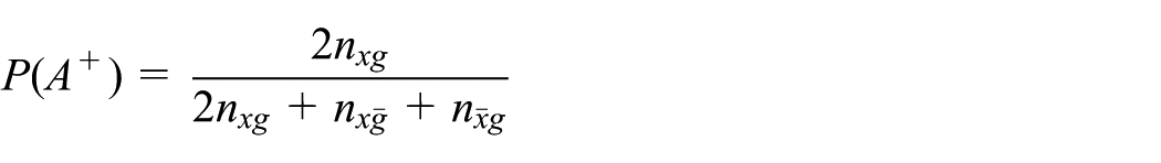
Positive agreement is interpreted as the conditional probability of agreement considering that one of the clustering definitions has already stated that the pair of sensors should be clustered together and is defined as

P (A^{+}) = \frac{2 n_{xg}}{2 n_{xg} + n_{x \bar{g}} + n_{\bar{x} g}}

From our point of view, this clearly relates to the proportion of agreement on compactness of the clustering structure, focusing on the pair of points that both clustering definitions state should be together.

Separability

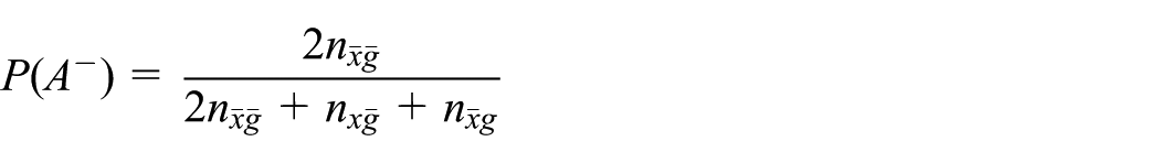
Negative agreement is interpreted as the conditional probability of agreement considering that one of the clustering definitions has already stated that the pair of sensors should be separated and is defined as

P (A^{-}) = \frac{2 n_{\bar{x} \bar{g}}}{2 n_{\bar{x} \bar{g}} + n_{x \bar{g}} + n_{\bar{x} g}}

From our point of view, this clearly relates to the proportion of agreement on separability of the clustering structure, focusing on the pair of points that both clustering definitions state should be separated.

Robustness to data incompleteness

In adverse settings, as deployed sensor networks, communication is not flawless. In any installation, packet loss is more or less probable. Given this, one outcome that we also assess in this exposure is the robustness of the system to communication incompleteness.

For a given network setup, with fixed number of sensors $(d = 128)$ and clusters $(k = 5)$ , we set a parameter $λ \in [0, 1]$ to the network, so that each transmission in the network is lost (i.e. not delivered) with probability $P (lost) = λ$ . The final average proportion of agreement $P (A)$ is evaluated and the evolution of this index is also monitored in the first iterations to assess the impact in convergence speed, over 10 different network configurations.

Communication reduction

The main outcome that local algorithms try to improve is communication. In our setting, we should assess whether our solution reduces the overall communication when compared to the amount that would be required if data were gathered centrally.

For each evaluated network setup, with fixed number of sensors $(d = 128)$ , the total number $T_{local}$ of messages transmitted per iteration is tracked and then compared with the number of messages that would need to be transmitted, with the best possible routing path, $T_{sink}$ , averaged over all possible choices for the sink or choosing either the best or the worst possible node. Results are evaluated for 10 different network configurations.

Global assessment

Globally, next section will try to answer the following research question: Can L2GClust deliver in terms of cluster sanity, validity, compactedness and separability, communication reduction and robustness to communication incompleteness, when compared to the centralized stream clustering procedure which uses all sensor data directly, if Gaussian data are produced at each node according to a given mean, which was randomly and uniformely sampled from a set of Gaussian clusters?

Each experimental run results in a learning curve for each validity index. Left plot of Figure 5 presents the evolution of the average $P (A)$ index (over all sensors), for one network with $d = 128$ , $k = 7$ , and $σ = 0.01$ . Following the strategy proposed in Gama et al.,³ the curve should be smoothed by applying the fading average to the computed value (right plot of Figure 5). The main point to stress is that the network converges, besides some small oscillation due to randomness of data being produced.

Figure 5.

Evolution of the average proportion of agreement between sensors and the global clustering definition (one experimental run with $k = 7$ , $d = 128$ , and $σ = 0.01$ ). Left plot presents the actual average proportion of agreement (over all sensors). Right plot presents the fading average (over time) of the average proportion of agreement.

Since for each data scenario (k, σ, and d) 10 runs are executed for each of the three configurations of the sensor network, results are presented as mean values (and the corresponding 95% confidence interval) over the 30 runs. Given the convergence empirical observation (different scenarios converge at different number of node interactions), we compare the means (over all runs) for the fading average of each measure at the end of each run.

Evaluation results

In this section, we present the empirical results obtained from the evaluation setup previously presented. First, in terms of the agreement to the global clustering and then considering robustness to data incompleteness and communication reduction.

Agreement with global clustering

Tables 1 and 2 present the complete set of results from which most of the following interpretations can be drawn. The first result to extract is that all scenarios passed the sanity check, as $\hat{κ}$ statistic is always positive (in fact, higher than 0.58).

Table 1.

Clustering validity results, in terms of $\hat{κ}$ statistic (sanity), global agreement (assessment), positive agreement (compactness), negative agreement (separability), and the percentage of nodes presenting total agreement (perfectness): mean and the 95% confidence interval are presented for each combination of ${k, σ, d}$ parameters, with $k = {2, 3, 4}$ , averaging results over 10 random datasets for each of the three different network configurations (30 runs).

k	$σ$	d	$\hat{κ}$		$P (A)$		$P (A^{+})$		$P (A^{-})$		$P (A) = 1$
k	$σ$	d	$\hat{μ}$	(95% CI)	$\hat{μ}$	(95% CI)	$\hat{μ}$	(95% CI)	$\hat{μ}$	(95% CI)	$\hat{μ}$	(95% CI)
		8	0.99	(0.98; 1.00)	0.99	(0.99; 1.00)	0.99	(0.99; 1.00)	1.00	(0.99; 1.00)	0.98	(0.96; 1.00)
		16	0.99	(0.97; 1.00)	0.99	(0.99; 1.00)	0.99	(0.99; 1.00)	0.99	(0.99; 1.00)	0.98	(0.95; 1.00)
	0.01	32	0.99	(0.98; 1.00)	1.00	(0.99; 1.00)	1.00	(0.99; 1.00)	0.99	(0.99; 1.00)	0.99	(0.98; 1.00)
		64	1.00	(1.00; 1.00)	1.00	(1.00; 1.00)	1.00	(1.00; 1.00)	1.00	(1.00; 1.00)	1.00	(1.00; 1.00)
		128	0.86	(0.78; 0.94)	0.93	(0.89; 0.97)	0.94	(0.90; 0.97)	0.92	(0.88; 0.97)	0.71	(0.55; 0.87)
		8	0.94	(0.89; 0.99)	0.97	(0.94; 0.99)	0.97	(0.94; 0.99)	0.97	(0.95; 1.00)	0.92	(0.85; 0.98)
		16	0.94	(0.89; 0.99)	0.97	(0.95; 0.99)	0.97	(0.95; 0.99)	0.97	(0.95; 0.99)	0.88	(0.79; 0.97)
2	0.05	32	0.88	(0.80; 0.96)	0.94	(0.91; 0.98)	0.95	(0.92; 0.98)	0.91	(0.86; 0.97)	0.80	(0.68; 0.91)
		64	0.88	(0.81; 0.94)	0.94	(0.91; 0.97)	0.94	(0.91; 0.97)	0.94	(0.90; 0.97)	0.64	(0.49; 0.79)
		128	0.71	(0.64; 0.79)	0.86	(0.82; 0.89)	0.86	(0.83; 0.90)	0.85	(0.80; 0.89)	0.32	(0.16; 0.48)
		8	0.81	(0.73; 0.88)	0.91	(0.87; 0.94)	0.91	(0.88; 0.95)	0.89	(0.85; 0.93)	0.73	(0.63; 0.83)
		16	0.86	(0.82; 0.91)	0.93	(0.91; 0.95)	0.93	(0.91; 0.95)	0.93	(0.91; 0.95)	0.63	(0.51; 0.74)
	0.10	32	0.73	(0.66; 0.80)	0.87	(0.83; 0.90)	0.88	(0.84; 0.91)	0.85	(0.81; 0.90)	0.35	(0.25; 0.46)
		64	0.67	(0.59; 0.75)	0.84	(0.80; 0.88)	0.85	(0.82; 0.88)	0.82	(0.77; 0.87)	0.20	(0.11; 0.29)
		128	0.55	(0.49; 0.60)	0.77	(0.75; 0.80)	0.79	(0.77; 0.81)	0.75	(0.72; 0.78)	0.02	(0.02; 0.03)
		8	0.91	(0.85; 0.97)	0.96	(0.93; 0.99)	0.94	(0.90; 0.98)	0.97	(0.95; 0.99)	0.82	(0.70; 0.95)
		16	0.97	(0.95; 1.00)	0.99	(0.98; 1.00)	0.98	(0.97; 1.00)	0.99	(0.98; 1.00)	0.92	(0.84; 1.00)
	0.01	32	0.95	(0.91; 0.99)	0.98	(0.96; 1.00)	0.97	(0.95; 0.99)	0.98	(0.96; 1.00)	0.82	(0.70; 0.93)
		64	1.00	(1.00; 1.00)	1.00	(1.00; 1.00)	1.00	(1.00; 1.00)	1.00	(1.00; 1.00)	1.00	(1.00; 1.00)
		128	0.90	(0.84; 0.95)	0.95	(0.92; 0.98)	0.94	(0.90; 0.97)	0.96	(0.93; 0.98)	0.71	(0.54; 0.87)
		8	0.95	(0.91; 0.99)	0.98	(0.96; 1.00)	0.97	(0.94; 0.99)	0.98	(0.97; 1.00)	0.93	(0.87; 0.98)
		16	0.86	(0.81; 0.91)	0.94	(0.91; 0.96)	0.91	(0.87; 0.94)	0.95	(0.93; 0.97)	0.59	(0.47; 0.70)
3	0.05	32	0.75	(0.71; 0.78)	0.88	(0.86; 0.90)	0.84	(0.82; 0.87)	0.90	(0.88; 0.92)	0.21	(0.10; 0.32)
		64	0.80	(0.76; 0.85)	0.91	(0.89; 0.93)	0.88	(0.85; 0.90)	0.93	(0.91; 0.94)	0.27	(0.15; 0.38)
		128	0.76	(0.70; 0.82)	0.89	(0.86; 0.91)	0.85	(0.82; 0.89)	0.91	(0.88; 0.93)	0.09	(0.05; 0.13)
		8	0.95	(0.93; 0.97)	0.98	(0.97; 0.99)	0.97	(0.95; 0.98)	0.99	(0.98; 0.99)	0.90	(0.86; 0.94)
		16	0.74	(0.69; 0.79)	0.88	(0.86; 0.90)	0.83	(0.80; 0.87)	0.91	(0.89; 0.92)	0.46	(0.38; 0.54)
	0.10	32	0.63	(0.58; 0.68)	0.83	(0.80; 0.85)	0.77	(0.74; 0.80)	0.86	(0.84; 0.88)	0.09	(0.04; 0.14)
		64	0.59	(0.57; 0.62)	0.81	(0.79; 0.82)	0.75	(0.73; 0.76)	0.84	(0.83; 0.86)	0.04	(0.02; 0.06)
		128	0.56	(0.54; 0.58)	0.79	(0.78; 0.80)	0.74	(0.73; 0.75)	0.82	(0.81; 0.83)	0.01	(0.00; 0.01)
		8	0.95	(0.91; 0.99)	0.98	(0.97; 1.00)	0.96	(0.93; 0.99)	0.99	(0.98; 1.00)	0.89	(0.80; 0.97)
		16	0.97	(0.95; 0.99)	0.99	(0.98; 1.00)	0.98	(0.96; 0.99)	0.99	(0.99; 1.00)	0.86	(0.77; 0.96)
	0.01	32	0.94	(0.91; 0.98)	0.98	(0.96; 0.99)	0.96	(0.94; 0.99)	0.98	(0.97; 0.99)	0.79	(0.66; 0.92)
		64	0.95	(0.91; 0.98)	0.98	(0.96; 0.99)	0.96	(0.94; 0.99)	0.98	(0.97; 0.99)	0.71	(0.55; 0.87)
		128	0.91	(0.87; 0.96)	0.96	(0.94; 0.98)	0.94	(0.90; 0.97)	0.97	(0.96; 0.99)	0.54	(0.39; 0.69)
		8	0.88	(0.84; 0.93)	0.96	(0.94; 0.98)	0.91	(0.87; 0.95)	0.98	(0.96; 0.99)	0.71	(0.59; 0.84)
		16	0.82	(0.78; 0.86)	0.93	(0.92; 0.95)	0.86	(0.83; 0.90)	0.96	(0.95; 0.97)	0.47	(0.36; 0.59)
4	0.05	32	0.78	(0.73; 0.82)	0.91	(0.89; 0.92)	0.84	(0.81; 0.87)	0.93	(0.92; 0.94)	0.18	(0.09; 0.28)
		64	0.73	(0.69; 0.76)	0.89	(0.87; 0.90)	0.81	(0.78; 0.83)	0.92	(0.91; 0.93)	0.04	(0.02; 0.06)
		128	0.66	(0.64; 0.68)	0.86	(0.85; 0.87)	0.76	(0.75; 0.78)	0.90	(0.89; 0.90)	0.00	(0.00; 0.00)
		8	0.93	(0.88; 0.98)	0.98	(0.96; 0.99)	0.94	(0.90; 0.98)	0.99	(0.98; 1.00)	0.85	(0.76; 0.94)
		16	0.81	(0.77; 0.85)	0.93	(0.91; 0.94)	0.85	(0.82; 0.89)	0.95	(0.94; 0.96)	0.40	(0.28; 0.52)
	0.10	32	0.69	(0.65; 0.73)	0.87	(0.85; 0.89)	0.78	(0.75; 0.81)	0.91	(0.89; 0.92)	0.06	(0.04; 0.08)
		64	0.67	(0.63; 0.72)	0.86	(0.85; 0.88)	0.77	(0.74; 0.80)	0.90	(0.89; 0.91)	0.01	(0.01; 0.02)
		128	0.59	(0.56; 0.61)	0.82	(0.81; 0.83)	0.72	(0.70; 0.74)	0.87	(0.86; 0.88)	0.00	(0.00; 0.00)

CI: confidence interval.

Table 2.

Clustering validity results, in terms of $\hat{κ}$ statistic (sanity), global agreement (assessment), positive agreement (compactness), negative agreement (separability), and the percentage of nodes presenting total agreement (perfectness): mean and the 95% confidence interval are presented for each combination of ${k, σ, d}$ parameters, with $k = {5, 6, 7}$ , averaging results over 10 random datasets for each of the three different network configurations (30 runs).

k	$σ$	d	$\hat{κ}$		$P (A)$		$P (A^{+})$		$P (A^{-})$		$P (A) = 1$
k	$σ$	d	$\hat{μ}$	(95% CI)	$\hat{μ}$	(95% CI)	$\hat{μ}$	(95% CI)	$\hat{μ}$	(95% CI)	$\hat{μ}$	(95% CI)
		8	0.94	(0.90; 0.98)	0.99	(0.98; 1.00)	0.95	(0.91; 0.98)	0.99	(0.99; 1.00)	0.85	(0.75; 0.95)
		16	0.95	(0.92; 0.97)	0.98	(0.97; 0.99)	0.96	(0.94; 0.98)	0.99	(0.98; 0.99)	0.83	(0.73; 0.92)
	0.01	32	0.95	(0.93; 0.97)	0.98	(0.98; 0.99)	0.96	(0.94; 0.98)	0.99	(0.98; 0.99)	0.66	(0.52; 0.80)
		64	0.93	(0.91; 0.96)	0.98	(0.97; 0.98)	0.95	(0.93; 0.97)	0.98	(0.98; 0.99)	0.44	(0.29; 0.60)
		128	0.87	(0.83; 0.91)	0.95	(0.94; 0.97)	0.90	(0.87; 0.93)	0.97	(0.96; 0.98)	0.29	(0.15; 0.43)
		8	0.86	(0.81; 0.90)	0.97	(0.95; 0.98)	0.88	(0.83; 0.92)	0.98	(0.97; 0.99)	0.72	(0.63; 0.81)
		16	0.84	(0.79; 0.88)	0.94	(0.92; 0.96)	0.87	(0.84; 0.91)	0.96	(0.95; 0.97)	0.46	(0.33; 0.59)
5	0.05	32	0.76	(0.73; 0.79)	0.92	(0.91; 0.93)	0.82	(0.80; 0.84)	0.95	(0.94; 0.95)	0.10	(0.04; 0.15)
		64	0.70	(0.67; 0.73)	0.89	(0.88; 0.90)	0.77	(0.75; 0.80)	0.93	(0.92; 0.93)	0.01	(0.00; 0.02)
		128	0.67	(0.65; 0.69)	0.88	(0.87; 0.89)	0.75	(0.74; 0.77)	0.92	(0.91; 0.92)	0.00	(0.00; 0.00)
		8	0.91	(0.86; 0.95)	0.98	(0.97; 0.99)	0.92	(0.88; 0.96)	0.99	(0.98; 0.99)	0.74	(0.60; 0.88)
		16	0.83	(0.81; 0.86)	0.94	(0.93; 0.95)	0.87	(0.85; 0.89)	0.96	(0.96; 0.97)	0.35	(0.25; 0.46)
	0.10	32	0.69	(0.65; 0.73)	0.89	(0.87; 0.90)	0.76	(0.73; 0.79)	0.93	(0.92; 0.94)	0.12	(0.05; 0.20)
		64	0.67	(0.64; 0.70)	0.87	(0.86; 0.88)	0.76	(0.74; 0.78)	0.91	(0.90; 0.92)	0.01	(0.00; 0.02)
		128	0.59	(0.58; 0.61)	0.84	(0.84; 0.85)	0.70	(0.69; 0.71)	0.89	(0.89; 0.90)	0.00	(0.00; 0.00)
		8	0.97	(0.94; 1.00)	1.00	(0.99; 1.00)	0.97	(0.95; 1.00)	1.00	(1.00; 1.00)	0.95	(0.89; 1.00)
		16	0.95	(0.92; 0.98)	0.99	(0.98; 0.99)	0.96	(0.93; 0.98)	0.99	(0.99; 1.00)	0.78	(0.66; 0.90)
	0.01	32	0.92	(0.89; 0.95)	0.97	(0.96; 0.98)	0.93	(0.91; 0.96)	0.98	(0.98; 0.99)	0.54	(0.37; 0.70)
		64	0.88	(0.84; 0.92)	0.96	(0.95; 0.98)	0.90	(0.87; 0.94)	0.98	(0.97; 0.99)	0.40	(0.26; 0.54)
		128	0.88	(0.86; 0.90)	0.96	(0.96; 0.97)	0.91	(0.89; 0.92)	0.98	(0.97; 0.98)	0.16	(0.04; 0.28)
		8	0.90	(0.84; 0.96)	0.99	(0.98; 1.00)	0.91	(0.85; 0.97)	0.99	(0.99; 1.00)	0.83	(0.73; 0.94)
		16	0.84	(0.80; 0.87)	0.95	(0.94; 0.96)	0.86	(0.83; 0.89)	0.97	(0.97; 0.98)	0.45	(0.36; 0.55)
6	0.05	32	0.81	(0.76; 0.85)	0.94	(0.93; 0.96)	0.84	(0.81; 0.88)	0.97	(0.96; 0.97)	0.24	(0.13; 0.35)
		64	0.72	(0.69; 0.75)	0.90	(0.89; 0.92)	0.78	(0.76; 0.81)	0.94	(0.93; 0.95)	0.02	(0.01; 0.02)
		128	0.63	(0.62; 0.65)	0.88	(0.87; 0.89)	0.71	(0.70; 0.72)	0.93	(0.92; 0.93)	0.00	(0.00; 0.00)
		8	0.92	(0.87; 0.97)	0.99	(0.98; 0.99)	0.92	(0.88; 0.97)	0.99	(0.99; 1.00)	0.86	(0.77; 0.94)
		16	0.76	(0.73; 0.80)	0.94	(0.92; 0.95)	0.80	(0.77; 0.83)	0.96	(0.95; 0.97)	0.20	(0.13; 0.27)
	0.10	32	0.72	(0.69; 0.76)	0.91	(0.90; 0.92)	0.78	(0.75; 0.81)	0.95	(0.94; 0.95)	0.11	(0.06; 0.16)
		64	0.65	(0.63; 0.68)	0.89	(0.88; 0.90)	0.73	(0.71; 0.75)	0.93	(0.92; 0.93)	0.01	(0.01; 0.02)
		128	0.61	(0.60; 0.63)	0.86	(0.86; 0.87)	0.70	(0.69; 0.71)	0.91	(0.91; 0.92)	0.00	(0.00; 0.00)
		8	0.83	(0.71; 0.94)	0.99	(0.98; 0.99)	0.83	(0.72; 0.95)	0.99	(0.99; 1.00)	0.70	(0.53; 0.87)
		16	0.96	(0.94; 0.98)	0.99	(0.99; 1.00)	0.96	(0.94; 0.98)	0.99	(0.99; 1.00)	0.80	(0.70; 0.91)
	0.01	32	0.92	(0.89; 0.95)	0.98	(0.97; 0.99)	0.93	(0.90; 0.96)	0.99	(0.98; 0.99)	0.59	(0.44; 0.74)
		64	0.87	(0.85; 0.90)	0.97	(0.96; 0.97)	0.89	(0.87; 0.91)	0.98	(0.98; 0.98)	0.17	(0.07; 0.27)
		128	0.85	(0.82; 0.87)	0.96	(0.95; 0.96)	0.87	(0.85; 0.89)	0.98	(0.97; 0.98)	0.07	(0.01; 0.12)
		8	1.00	(1.00; 1.00)	1.00	(1.00; 1.00)	1.00	(1.00; 1.00)	1.00	(1.00; 1.00)	1.00	(0.99; 1.00)
		16	0.85	(0.82; 0.89)	0.97	(0.96; 0.97)	0.87	(0.84; 0.90)	0.98	(0.98; 0.98)	0.43	(0.30; 0.55)
7	0.05	32	0.77	(0.74; 0.80)	0.94	(0.92; 0.95)	0.81	(0.78; 0.84)	0.96	(0.95; 0.97)	0.09	(0.04; 0.14)
		64	0.70	(0.67; 0.72)	0.91	(0.90; 0.92)	0.75	(0.73; 0.77)	0.95	(0.94; 0.95)	0.00	(0.00; 0.00)
		128	0.66	(0.64; 0.67)	0.89	(0.89; 0.90)	0.72	(0.71; 0.74)	0.93	(0.93; 0.94)	0.00	(0.00; 0.00)
		8	0.93	(0.88; 0.97)	0.99	(0.99; 1.00)	0.93	(0.89; 0.97)	1.00	(0.99; 1.00)	0.84	(0.72; 0.96)
		16	0.83	(0.80; 0.87)	0.96	(0.96; 0.97)	0.85	(0.82; 0.88)	0.98	(0.97; 0.98)	0.41	(0.31; 0.51)
	0.10	32	0.74	(0.71; 0.77)	0.93	(0.93; 0.94)	0.78	(0.76; 0.81)	0.96	(0.96; 0.97)	0.05	(0.03; 0.08)
		64	0.65	(0.63; 0.67)	0.90	(0.89; 0.90)	0.72	(0.70; 0.73)	0.94	(0.93; 0.94)	0.00	(0.00; 0.01)
		128	0.59	(0.58; 0.60)	0.87	(0.86; 0.87)	0.67	(0.67; 0.68)	0.92	(0.91; 0.92)	0.00	(0.00; 0.00)

CI: confidence interval.

After confirming the sanity of our approach, we can stress that a high level of average agreement is achieved for most of the scenarios. Focusing on the lower limits of the 95% confidence intervals, $P (A) \geq 75 %$ , with $66 %$ of scenarios with $P (A) \geq 90 %$ . Moreover, for the theoretically hardest scenario presented here ( $k = 7$ , $σ = 0.10$ , and $d = 128$ ), the lower limit of the confidence interval is $P (A) = 0.86$ , meaning that, on average, a sensor node would agree with the global clustering on over $86 %$ of the total pairs of sensors.

Regarding the direction of agreement, we should stress that our approach clearly gives more relevance to separability. In all scenarios where the average proportion of positive agreement (compactness) is different (under the 95% confidence level) from the average proportion of negative agreement (separability), the separability index is always higher than the compactness index.

Moreover, even for scenarios with lower average proportion of agreement, separability tends to stay high ( $P (A^{-}) \geq 81 %$ , with $81 %$ of scenarios with $P (A^{-}) \geq 90 %$ ), meaning that in our approach, each single node will have a high level of agreement on answer queries for which pairs of nodes should be clustered separately than on queries for which pairs of nodes should be clustered together. Worse results appear for compactness agreement, as $P (A^{+}) \geq 0.67$ , with only $37 %$ of scenarios with $P (A^{+}) \geq 90 %$ .

Finally, it became clear that at least for harder scenarios, it is very difficult to achieve networks where all nodes agree with central clustering on 100% of pairs of nodes. From our observation, this might result from different node connectivity (nodes placed on the outer ribbon of the network could have more difficult to converge to global clustering). Nevertheless, results put the agreement at a high level, stating that local clustering gives a good approximation of the global clustering.

Robustness to data incompleteness

Figure 6 presents the average proportion of agreement for the evaluated setups, averaged over 10 runs, and the corresponding 95% confidence intervals. Although the setting is one of the hardest that was studied in this evaluation ( $d = 128$ sensors and $k = 5$ clusters), the reader can note that only for high levels of communication incompleteness (probability of message loss above $λ = 0.95$ for $σ = 0.01$ , $λ = 0.97$ for $σ = 0.05$ , and $λ = . 85$ for $σ = 0.1$ ) we can state that final agreement is harmed by communication incompleteness, with statistical significance under the 0.05 significance level.

Figure 6.

Impact of communication incompleteness on average proportion of agreement. Lines represent the average result of 10 runs for each setup ( $k = 5$ , $d = 128$ , $σ \in {0.01, 0.05, 0.1}$ , and $λ \in [0, 1]$ ), with the error bars representing the 95% confidence interval.

Given the stability of the studied scenarios, and for at least a reasonable quality of service, it is expected that following transmissions should compensate the lost messages. However, we expect that the speed of convergence will be more sensitive to message lost. For the same setup, Figure 7 presents the evolution of the average proportion of agreement, at the very beginning of each run, for each level of communication incompleteness. The reader can note that, as expected, although at the end there might not be a difference in the agreement (besides extremely high levels of incompleteness), there is a difference in the speed at which the system converges to that level of agreement.

Figure 7.

Impact of communication incompleteness on the evolution of the average proportion of agreement. Lines represent the average result of 10 runs for each setup ( $k = 5$ , $d = 128$ , $σ \in {0.01, 0.05, 0.1}$ , and $λ \in [0, 1]$ ), with the error bars representing the 95% confidence interval (logarithmic x-axis; cubic y-axis; darker lines represent higher $λ$ values).

Communication reduction

Figure 8 presents the estimates of the average number of hops that messages need to traverse in order to reach the sink. Our objective was to show the average number of point-to-point data transmissions that the system would need to perform so that a single message containing the data of one node could reach the sink. We do this in three different scenarios where the sink is chosen as the best possible one, the worst possible one, and on average, all in a randomly generated network of 128 nodes. The reader can note that even if the deployment enables a perfect routing path, and the definition of the best possible sink node is possible, in the evaluated scenario the average number of hops to the sink is 4. Hence, the local-to-global communication ratio for $d = 128$ is $1 / 4$ .

Figure 8.

Average number of hops to sink, for networks with $d = 128$ , when the sink is chosen as the best one, $\min ({\bar{P}}_{x})$ , on average, $avg ({\bar{P}}_{x})$ , or the worst possible node, $\max ({\bar{P}}_{x})$ . Estimates of the mean are presented, with error bars representing the 95% confidence interval estimated over 10 generated networks.

Certainly, the local approach must send multiple-valued messages (actually, k values per message), while the global solution sends single-valued messages. In terms of the number of transmitted values, only for scenarios where $k \geq 4$ , the benefits fade for networks with $d = 128$ . Nonetheless, we should stress that sending a message with k values is certainly less resource-expensive than sending k messages of a single value. This way, we argue that local algorithms present advantages in terms of communication even when $k > {\bar{P}}_{x}$ . Also, the impact of a badly chosen sink in communication resources is clear, which is otherwise completely irrelevant in local algorithms.

Sensitivity to the number of sensors

Figure 9 presents an average assessment of the quality of the proposal, with the analysis of sensitivity according to different number and overlap of clusters, for an increasing number of sensors. A more detailed analysis on sensitivity to network configuration is out of the scope of this presentation. However, we can argue that agreement levels are robust to an increase in the number of clusters, being, however, a bit more sensitive with respect to network size ( $P (A)$ decreases when d increases) and cluster overlapping ( $P (A)$ decreases when $σ$ increases). This effect is observed also for the other indices. Given the comparison between $P (A^{+})$ and $P (A^{-})$ , we can conclude that it is the extra sensitivity of the compactness agreement that decreases the quality of the overall agreement, enhancing its sensitivity to the aforementioned parameters.

Figure 9.

Sensitivity of $\hat{κ}$ , $P (A)$ , $P (A +)$ , $P (A -)$ , and $P (A) = 1$ to the number of sensors, according to different number and overlap of clusters. Left plots present the impact of the number of sensors (from $d = 8$ to $d = 128$ ) for each overlap (from $s = 0.01$ to $s = 0.10$ ), estimated over all values of k (from $k = 2$ to $k = 6$ ). Error bars represent the 95% confidence interval estimated using pooled variances. Right plots present the same results but for each value of k, estimated over all values of s.

Real data from electricity sensors

Real data are never clean, and half of the sensors have more than $27 %$ missing values, which naturally hindered the analysis. Given this, and the dynamic nature of the data, no convergence was possible in the clustering structures. However, we could stress that as more data are being fed to the system, better agreement can be achieved with the centralized approach, as exposed in Figure 10. Further experiments should focus only on those sensors from which good information can be extracted, so that a deeper analysis can be performed.

Figure 10.

Experimental results. Evolution of clustering agreement for a real active power sensor data log, where not only does the agreement tend to increase with more observations, but also changes on the clustering structure are apparently possible to detect.

Limitations and future work

Averages can be viewed as the values minimizing quadratic cost functions, hence there is relevance in monitoring average values. However, in streaming settings, deeper sketches are often needed. The convergence and validity properties of an extension of L2GClust to online histograms or other sketches are still to be proved. Also, asynchronous processing is often (if not always) the case in sensor networks. Other scenarios are also prone to synchronousness issues. Although the proposed local algorithm seems robust in those settings, a deeper evaluation of this issue is required.

If the concept of the data being produced in the network is stable, then the clustering estimates will converge, and transmissions will become redundant. We should include mechanisms to allow each sensor to decide to which neighbors it is still valuable to send information. However, the world is not static. It is possible that with time, the sketches of each sensor will change, adapting to new concepts of data. On a long run, the communication management strategy could prevent the system from adapting to new data. Sensors should include change detection⁴⁵ mechanisms that would trigger if the data change, either univariately at each sensor or in the global interaction of sensors.

As possible extension, since each node clusters its neighbors’ centroids as single points, the node could fit a clustering definition with different number of clusters. Moreover, it could fit three clustering definitions (e.g. with $k = K$ , $k = K - 1$ , and $k = K + 1$ clusters) and test which of them is better using, for example, the Davies–Bouldin index,⁸ a clustering validity measure that can be used to infer the appropriateness of data partitions and can therefore be used to compare relative appropriateness of various divisions of the data, being thus useful to guide a cluster-seeking algorithm, having the positive characteristic of not depending on the number of clusters, hence enabling the comparison of clusterings with different k. For example, if a node decides that it should start fitting $k = K + 1$ clusters instead, it would then start fitting $k = K$ , $k = K + 1$ , and $k = K + 2$ , hence monitoring cluster evolution. This is targeted for future developments of the L2GClust algorithm.

The analysis on whether the quality of the local clusterings are related with their position in the network should be addressed in future work. It seems reasonable to expect that edge sensors have lower quality than central sensors, but this was not assessed. Also, internal validity indices should be used to assess the quality of a given local clustering, since no external comparison is possible in real world. Furthermore, the implementation on real sensors should be evaluated soon in a laboratorial environment.

Findings and recommendations

A local algorithm was proposed to perform clustering of sensors on ubiquitous sensor networks, based on the moving average of each node’s data over time. There are two main characteristics. On one hand, each sensor node keeps a sketch of its own data. On the other hand, communication is limited to direct neighbors, so clustering is computed at each node. The moving average of each node is approximated using memoryless fading average, while clustering is based on the furthest-point algorithm applied to the centroids computed by the node’s direct neighbors. Each sensor acts not only as a data stream source but also as a processing node, keeping a sketch of its own data and a definition of the clustering structure of the entire network of data sources.

From our empirical observations, we can argue that performing local clustering at each node, without a centralized server aggregating data from the network, is a valuable approximation of the global clustering that a centralized algorithm would gather. Local algorithms present an extremely high level of agreement with the global clustering, especially in terms of separability agreement: if according to the global clustering two nodes should be separated, local approximations will also state that with high probability. Moreover, the results on stable concepts are robust to communication incompleteness, supporting its application in adverse settings such as sensor networks. Furthermore, the gain in communication by disregarding a routing path and forwarding schema seems an important resource booster.

Even though processing may be concentrated on local computations and short-range communication, the final goal is to infer a global clustering structure of all relevant sensors. Hence, approximate algorithms should be considered to prevent global data transmission. Given this, when querying a given sensor for the global clustering, we allow (and known beforehand that we will have) an approximate result within a maximum possible error with a certain probability. Each approximation step (local sketch, local clustering update, merging different cluster definitions, etc.) should be restricted by some stability bound on the error.⁴⁶ These bounds should serve as balancing deciders in the trade-off between transmission management and resulting errors.

Moreover, if the concept of the data being produced in the network is stable, then the clustering estimates will converge, and transmissions will become redundant. We should include mechanisms to allow each sensor to decide to which neighbors it is still valuable to send information. However, the world is not static. It is possible that with time, the sketches of each sensor will change, adapting to new concepts of data. On a long run, the communication management strategy could prevent the system from adapting to new data. Sensors should include change detection mechanisms that would trigger if the data change, either univariately at each sensor or in the global interaction of sensor data.

We have presented a local algorithm to cluster ubiquitous streaming data sources produced in distributed sensor network settings. The proposed local clustering algorithm presents high level of agreement with a global clustering algorithm which could have been run in a centralized fashion, while reducing communication throughout the network and being robust to communication incompleteness. This local approach brings benefits for real-world applications and sensor networks, creating a research path with near-future improvements and applications, which enables the improvement of sensor deployment, might reduce message forwarding, preserves privacy of observed data, and improves network comprehension, in the sense that each sensor is able to tell where in the sensor data domain it is located.

Footnotes

Acknowledgements

This work has been developed under the scope of projects Nano STIMA (NORTE-01-0145-FEDER-000016) and SMILES (NORTE-01-145-FEDER-000020), both financed by the North Portugal Regional Operational Program (NORTE 2020), under the PORTUGAL 2020 Partnership Agreement and through the European Regional Development Fund (ERDF).

Handling Editor: Amiya Nayak

Declaration of conflicting interests

The author(s) declared no potential conflicts of interest with respect to the research, authorship, and/or publication of this article.

Funding

The author(s) disclosed receipt of the following financial support for the research, authorship, and/or publication of this article: This publication has been financed by project NanoSTIMA (NORTE-01-0145-FEDER-000016) which was financed by the North Portugal Regional Operational Program (NORTE 2020) under the PORTUGAL 2020 Partnership Agreement and through the European Regional Development Fund (ERDF).

ORCID iDs

Pedro Pereira Rodrigues

João Gama

References

Rodrigues

Gama

Distributed clustering of ubiquitous data streams. WIREs Data Min Knowl 2014; 4(1): 38–54.

Rodrigues

Gama

Clustering techniques in sensor networks. In: Gama

Gaber

(eds) Learning from data streams—processing techniques in sensor networks, chapter 9. Berlin: Springer, 2007, pp.125–142.

Gama

Sebastiao

Rodrigues

PP.

On evaluating stream learning algorithms. Mach Learn 2013; 90(3): 317–346.

Wang

Cao

et al . Particle swarm optimization based clustering algorithm with mobile sink for WSNs. Future Gener Comp Sy 2017; 76: 452–457.

Kargupta

Park

Pittie

et al . MobiMine: monitoring the stock market from a PDA. SIGKDD Explor News 2002; 3(2): 37–46.

Rodrigues

Gama

Lopes

. Knowledge discovery for sensor network comprehension. In: Cuzzocrea

(ed.) Intelligent techniques for warehousing and mining sensor network data, chapter 6. Hershey, PA: IGI Global, 2010, pp.118–135.

Gaber

Zaslavsky

Krishnaswamy

Resource-aware knowledge discovery in data streams. In: Aguilar-Ruiz

Gama

(eds) Proceedings of the 1st international workshop on knowledge discovery in data streams (ECML/PKDD), Pisa, Italy, 20–24 September 2004, pp.32–44. ECML/PKDD.

Halkidi

Batistakis

Varzirgiannis

On clustering validation techniques. J Intell Inform Syst 2001; 17(2–3): 107–145.

Aggarwal

Han

Wang

et al . A framework for clustering evolving data streams. In: Proceedings of the 29th international conference on very large data bases, Berlin, 9–12 September 2003, pp.81–92. Berlin, Germany: Morgan Kaufmann Publishers.

10.

Barbará

Requirements for clustering data streams. SIGKDD Explor News 2002; 3(2): 23–27.

11.

Rodrigues

Gama

Pedroso

JP.

Hierarchical clustering of time-series data streams. IEEE T Knowl Data En 2008; 20(5): 615–627.

12.

Beringer

Hüllermeier

Fuzzy clustering of parallel data streams. Data Knowl Eng 2006; 58(2): 333–352.

13.

Dai

Huang

Yeh

et al . Adaptive clustering for multiple evolving streams. IEEE T Knowl Data En 2006; 18(9): 1166–1180.

14.

Chan

Luk

Perrig

. Using clustering information for sensor network localization. In: Proceedings of the 1st international conference on distributed computing in sensor systems, Marina del Rey, CA, 30 June–1 July 2005, pp.109–125. New York: IEEE.

15.

Garg

Shyamasundar

RK.

A distributed clustering framework in mobile ad hoc networks. In: Proceedings of the international conference on wireless networks, Las Vegas, NV, 21–24 June 2004, pp.32–38. CSREA Press.

16.

Younis

Fahmy

HEED: a hybrid, energy-efficient, distributed clustering approach for ad hoc sensor networks. IEEE T Mobile Comput 2004; 3(4): 366–379.

17.

Ibriq

Mahgoub

Cluster-based routing in wireless sensor networks: issues and challenges. In: Proceedings of the international symposium on performance evaluation of computer and telecommunication systems, San Jose, CA, 25–29 July 2004, pp.759–766. SCS.org.

18.

Rodrigues

Gama

Lopes

. Requirements for clustering streaming sensors. In: Ganguly

Gama

Omitaomu

et al . (eds) Knowledge discovery from sensor data, chapter 4 (Industrial Innovation Series). Boca Raton, FL: CRC Press, 2008, pp.35–53.

19.

Kargupta

Huang

Sivakumar

et al . Distributed clustering using collective principal component analysis. Knowl Inform Syst 2001; 3(4): 422–448.

20.

Cormode

Muthukrishnan

Zhuang

. Conquering the divide: continuous clustering of distributed data streams. In: Proceedings of the 23rd international conference on data engineering, Istanbul, Turkey, 15–20 April 2007, pp.1036–1045. New York: IEEE.

21.

Datta

Bhaduri

Giannella

et al . Distributed data mining in peer-to-peer networks. IEEE Internet Comput 2006; 10(4): 18–26.

22.

Gaber

. A framework for resource-aware knowledge discovery in data streams: a holistic approach with its application to clustering. In: Proceedings of the symposium on applied computing, Dijon, 23–27 April 2006, pp.649–656. New York: ACM.

23.

Klusch

Lodi

Moro

. Distributed clustering based on sampling local density estimates. In: Proceedings of the 18th international joint conference on artificial intelligence, Acapulco, Mexico, 9–15 August 2003, pp.485–490. New York: ACM.

24.

Bandyopadhyay

Giannella

Maulik

et al . Clustering distributed data streams in peer-to-peer environments. Inform Sci 2006; 176(14): 1952–1985.

25.

Yin

Gaber

Clustering distributed time series in sensor networks. In: Proceedings of the 8th international conference on data mining, Pisa, 15–19 December 2008, pp.678–687. New York: IEEE.

26.

Rodrigues

Gama

A system for analysis and prediction of electricity-load streams. Intell Data Anal 2009; 13(3): 477–496.

27.

Sun

Sauvola

. Towards advanced modeling techniques for wireless sensor networks. In: Proceedings of the 1st international symposium on pervasive computing and applications, Urumqi, China, 3–5 August 2006, pp.133–138. New York: IEEE.

28.

Moreira

Santos

. Enhancing a user context by real-time clustering mobile trajectories. In: Proceedings of the international conference on information technology: coding and computing, vol. 2, Las Vegas, NV, 4–6 April, p.836. Los Alamitos, CA: IEEE Computer Society.

29.

Zhang

Torkkola

et al . A context aware automatic traffic notification system for cell phones. In: Proceedings of the 27th international conference on distributed computing systems workshops, Toronto, ON, Canada, 22–29 June 2007, pp.48–50. New York: IEEE.

30.

Sherrill

Moy

Reilly

et al . Using hierarchical clustering methods to classify motor activities of COPD patients from wearable sensor data. J Neuroeng Rehabil 2005; 2: 16.

31.

Barbará

Chen

. Using the fractal dimension to cluster datasets. In: Proceedings of the 6th SIGKDD international conference on knowledge discovery and data mining, Boston, MA, 20–23 August 2000, pp.260–264. New York: ACM.

32.

Wolff

Bhaduri

Kargupta

A generic local algorithm for mining data streams in large distributed systems. IEEE T Knowl Data En 2009; 21(4): 465–478.

33.

Rabbat

Nowak

Distributed optimization in sensor networks. In: Proceedings of the 3rd international symposium on information processing in sensor networks, Berkeley, CA, 27 April 2004, pp.20–27. New York: IEEE.

34.

Gama

Rodrigues

PP.

Data stream processing. In: Gama

Gaber

(eds) Learning from data streams—processing techniques in sensor networks, chapter 3. Berlin: Springer, 2007, pp.25–39.

35.

Rodrigues

Gama

Sebastião

. Memoryless fading windows in ubiquitous settings. In: Proceedings of the 1st ubiquitous data mining workshop, Lisbon, Portugal, 16–20 August, pp.23–27. ECCAI.

36.

Berthold

Hand

Intelligent data analysis—an introduction. Berlin, Germany: Springer-Verlag, 1999.

37.

Gonzalez

TF.

Clustering to minimize the maximum inter-cluster distance. Theor Comput Sci 1985; 38: 293–306.

38.

Eker

Janneck

Lee

et al . Taming heterogeneity: the Ptolemy approach. Proc IEEE 2003; 91(1): 127–144.

39.

Baldwin

Kohli

Lee

et al . Modelling of sensor nets in Ptolemy II. In: Proceedings of the 3rd international symposium on information processing in sensor networks, Berkeley, CA, 27 April 2004, pp.359–368. New York: ACM.

40.

Domingos

Hulten

. A general method for scaling up machine learning algorithms and its application to clustering. In: Proceedings of the 18th international conference on machine learning, Williamstown, MA, 28 June–1 July 2001, pp.106–113. New York: ACM.

41.

Jain

Dubes

RC.

Algorithms for clustering data. Englewood Cliffs, NJ: Prentice-Hall, 1988.

42.

Cohen

A coefficient of agreement for nominal scales. Educ Psychol Meas 1960; 20: 37–46.

43.

Fleiss

Levin

Paik

MC.

Statistical methods for rates and proportions. Hoboken, NJ: Wiley-InterScience, 2003.

44.

Warrens

MJ.

On the equivalence of Cohen’s kappa and the Hubert-Arabie adjusted rand index. J Classif 2008; 25(2): 177–183.

45.

Gama

Medas

Castillo

et al . Learning with drift detection. In: Bazzan

ALC

Labidi

(eds) Advances in artificial intelligence (Lecture Notes in computer science), vol. 3171. Berlin: Springer, 2004, pp.286–295.

46.

Hoeffding

Probability inequalities for sums of bounded random variables. J Am Stat Assoc 1963; 58(301): 13–30.

A local algorithm to approximate the global clustering of streams generated in ubiquitous sensor networks

Abstract

Keywords

Introduction

Rationale

Clustering data-stream sources

Distributed clustering of streaming sources

Advantages of application

On real-world domains

On sensor network management

On sensor network comprehension

L2GClust—local-to-global clustering

Local data stream sketches

Memory-less fading average

Impact on ubiquitous processing

Local clustering of stream sources

Dissimilarity measure

Neighborhood communication

Neighborhood ensemble

Furthest-point clustering

Algorithm overview

Space, time, and communication complexity

Evaluation methodology

Simulation environment

The data actor

The sensor actor

The sink actor

Evaluated scenarios

Description of artificial data

Description of real electricity demand data

Description of simulated networks

Studied parameters

Comparison

Measured outcomes

Agreement as quality assessment

Sanity

Validity

Compactness

Separability

Robustness to data incompleteness

Communication reduction

Global assessment

Evaluation results

Agreement with global clustering

Robustness to data incompleteness

Communication reduction

Sensitivity to the number of sensors

Real data from electricity sensors

Limitations and future work

Findings and recommendations

Footnotes

Acknowledgements

Declaration of conflicting interests

Funding

ORCID iDs

References