Sage Journals: Discover world-class research

Abstract

With the advance in mobile network-based systems, dynamic system has become one of the hotspots in fundamental study of distributed systems. In this article, we consider the dynamic system with frequent topology changes arising from node mobility or other reasons, which is also referred to as “dynamic network.” With the model of dynamic network, fundamental distributed computing problems, such as information dissemination and election, can be formally studied with rigorous correctness. Our work focuses on the node counting problem in dynamic environments. We first define two new dynamicity models, named (Q, S)-distance and (Q, S)*-distance, which describe dynamic changes of information propagation time against topology changes. Based on these two models, we design three different counting algorithms which basically adopt the approach of diffusing computation. These algorithms mainly differ in communication cost due to different information collection procedures. The correctness of all the algorithms is formally proved and their performance is evaluated via both theoretical analysis and experimental simulations.

Keywords

Node counting dynamic systems dynamic networks distributed algorithms system model

Introduction

In recent years, many efforts have been devoted to the study of dynamic distributed systems. Dynamic system is an abstraction of an adversary that controls the topology of the network, including peer-2-peer and mobile ad hoc systems. The dynamicity of dynamic systems lies in frequent topology changes due to node mobility^1,2 and/or changes of node set due to node joining/leaving.³ A dynamic system focusing on topology changes is also referred to as “dynamic network.”^4,5

Quite a lot of work has been done for dynamic networks. Researchers have proposed formal system models^6,7 to describe the change of network topology and distributed algorithms^8–10 with formal correctness proof to solve fundamental computing problems in dynamic environments.

Counting is one of fundamental problems in distributed computing, which concerns how to calculate the network size, that is, the number of nodes in the network.^1,11 Counting is the building block of many distributed computing problems. For example, in all-to-all information dissemination, knowing the number of nodes may be necessary.¹²

However, due to node mobility and limited connection, counting in dynamic networks becomes more challenging than in static networks. Quite a number of counting algorithms have been designed for dynamic networks.^1,2,11–13 Most of the existing algorithms are estimation-based, which may be efficient in terms of the cost of operations, especially in large networks. However, the counting results are not accurate. For example, the network size is estimated based on node degree and hop distance.² These algorithms can be used in scenarios that do not require accurate count values. Several accurate counting algorithms have been proposed.^7,14,15 Roughly, a non-deterministic algorithm is an algorithm that, even for the same input, can exhibit different behaviors on different runs, as opposed to a deterministic algorithm. The randomized estimation methods can always terminate, but in a non-deterministic way.

To achieve accurate counting results deterministically, we propose our new design for counting in dynamic networks. Basically, we adopt the diffusing computation,^16,17 a fundamental and classical approach in distributed computing to aggregate information of a distributed system. However, the basic/original diffusing computation algorithm is designed for static environments. In dynamic networks, due to topology dynamicity, the growing phase cannot terminate correctly and messages from children to parent cannot be successfully delivered.

After analyzing the effect of topology changes on diffusing computation, we first propose two new dynamicity models, called (Q, S)-distance and (Q, S)*-distance, which are defined to describe the change of distance between a pair of nodes. The first model is defined for any pair of nodes, while the second model is for neighboring nodes. Compare with existing dynamic models, different perspective is considered in these two models, that is, the change of dynamic distance.

Existing counting algorithms are not suitable for (Q, S)-distance model. Thus, based on the (Q, S)-distance model and (Q, S)*-distance model, we design three counting algorithms for dynamic networks. The first algorithm focuses on extending typical diffusing computation approach with mechanisms handling new challenges in dynamic environments. The major extension lies in a new phase to terminate the growing phase and invoke the shrinking phase.

The second algorithm improves the first algorithm by removing the messages to notify initiator node about the round that the last node joins the diffusing tree. Compared with the first algorithm, the second one can terminate Phase I earlier and cost fewer messages.

The third algorithm considers cluster-based hierarchy in counting operations. Clustering has been widely used to reduce communication cost in technical study of wireless networks^18–20 and also was recently considered in theoretical work, including consensus protocols²¹ and information dissemination algorithms.²² However, cluster hierarchy has not been considered for counting in dynamic networks. With the cluster hierarchy, diffusing computation may be conducted among only clusterhead nodes, and communication cost will be significantly reduced. The major challenge of hierarchical counting lies in the dynamic changes of cluster membership. By addressing such issues, we extend our flat counting algorithms to hierarchical ones.

The correctness of all the algorithms is rigorously proved, in terms of termination and correctness. To evaluate the performance of our algorithms, we conduct both theoretical analysis and experimental simulations. Both time cost in terms of communication rounds and message cost in terms of total size of messages sent by all nodes are measured and discussed.

The rest of the article is organized as follows. Section “Related work” briefly reviews existing works for dynamic networks, including system models and counting algorithms. We also introduce in this section the typical diffusing computation approach and discuss the major problems and challenges in applying it into dynamic networks. Section “System model and problem definition” presents system models and assumptions. The (Q, S)-distance model and (Q, S)*-distance model are defined in section “The (Q, S)-distance model and (Q, S)*-distance model.” Our three proposed algorithms are presented in sections “Algorithm 1—the basic algorithm for counting in a flat network,”“Algorithm 2—the improved algorithm for counting in a flat network,” and “Algorithm 3—the algorithm for counting in a hierarchical network,” respectively, together with correctness proof and communication cost analysis. Simulation results are reported in section “Simulation results.” Finally, section “Conclusion and future work” concludes the article with future directions.

Related work

In this section, we first introduce existing dynamic network models and then review existing counting algorithms for dynamic networks. Since our design is based on diffusing computation, which is not used before in counting for dynamic networks, we briefly introduce the typical diffusing computation algorithm in the end of this section and discuss challenges brought by topology dynamicity.

Dynamic network models

Network model is the basis of dynamic network research. Most existing dynamic network models focus on how to represent a dynamic network and they are usually extensions of the classical graph model G(V, E) by adding reflection of topology dynamicity.^5,6,23 The temporal network model (G, λ) is proposed in Kempe et al.⁶ and Berman,²⁴ where λ is the time label specifying at which time an edge e is available. The temporal network model is viewed as a sequence of graphs in Erlebach et al.,²⁵ and the edge-time pair (e, i) is used to denote the existence of e at time i. Akrida et al.²⁶ studied the temporal diameter of the directed random temporal graph model for the case of r = n. Grindrod and Higham²⁷ introduce a class of evolving range-dependent random graphs that gives a tractable framework for modeling and simulation. The notion of edge-Markovian dynamic graph is proposed by Clementi et al.,⁵ which refers to stochastic edge time-dependency in evolving graphs. Time-varying graph (TVG), proposed by Casteigts et al.,²³ integrates previous dynamic graph models with a unified framework. With TVG, a dynamic network is modeled as G = (V, E, T, ρ, ζ), where V and E are the vertex and edges in the topology graph, respectively; T is the lifetime of the network; ρ indicates whether a given edge is available; and ζ represents the time taken to cross an edge. A new unifying model for representing finite discrete TVGs is proposed in Wehmuth et al.,²⁸ which can capture the needs of distinct dynamic networks. Ducourthial and Wade²⁹ propose dynamic p-graphs model, which constituting a finite set of dynamic graphs and each of them being a sequence of observed graphs, with the particularity that their edges allow transferring p messages.

Besides network representation, researchers also consider the connectivity of dynamic networks and proposed different models. Kuhn and Oshman³⁰ propose the notion of “dynamic distance” between two nodes, which is the time required for one node to be causally influenced by the other node. Accordingly, the minimum upper bound on the distance between any pair of nodes is the “dynamic diameter.” The dynamic diameter extends the notion of normal diameter of a graph with consideration of dynamic changes. Kuhn et al.¹² propose the T-interval connected model, which requires that, for every T rounds, there exists a connected subgraph which keeps unchanged.

Our dynamicity models (Q, S)-distance model and (Q, S)*-distance model are defined on top of the notion of dynamic diameter and T-interval connectivity.

Dynamic counting algorithms

The counting problem has been widely studied under various environments. However, most counting algorithms for dynamic networks are based on estimation and the results are not accurate. Moreover, randomized design is usually adopted to cope with dynamicity, and the algorithms cannot terminate deterministically.

The algorithms in Psaltoulis et al.² and Kostoulas et al.¹³ adopt a random report approach. An initiator spreads messages to others and the receiver send replies randomly with some probability. The networks size, that is, the number of nodes, is estimated based on the number of replies and their corresponding hop distance.

Matias and Miele³¹ study statistical clustering. They explore statistical properties and deterministic inference in a model that combines a stochastic block model for its static part with independent Markov chains for the evolution of the nodes groups through time.

Massoulie et al.³² propose a random tour method where a node sends a node sample uniformly at random. They propose sample and collide method which relies on a sampling sub-routine that returns randomly chosen nodes.

The Degree_Counting algorithm in Michail et al.¹ calculates the degree of a node via broadcasting, and the network size is estimated by an upper bound on the maximum degree. Kuhn et al.¹² propose to do counting through k-committee election, where each committee invites no more than k nodes to join in, and the network size n is estimated to be k once k ≥ n.

All the algorithms above are estimation-based and cannot get accurate results.

Accurate algorithms can be found in De Bovenkamp et al.⁷ and Jelasity and colleagues.^14,15 These algorithms realize counting via token collection. Each node is assigned one token (or some information with unique copy) in the beginning and then periodically exchanges information with one of its neighbors to collect tokens from others. With delicately designed rules for token transferring, all the tokens will be eventually collected by one node, and the number of tokens collected is just the number of nodes in the network. These algorithms differ mainly in the mechanisms to direct and control the token aggregation procedure. Obviously, these algorithms are also randomized and cannot terminate deterministically. Moreover, the assumption of token information may not be acceptable in all application scenarios.

Michail et al.¹ also propose four accurate algorithms. The Fair algorithm and the Delegate algorithm are randomized. They count the number of nodes by naming the nodes with unique ID. In the Fair algorithm, the leader node assigns names to nodes it encounters and at the same time counting them. In the Delegate algorithm, the leader delegates the role of assigning names to all the nodes that it encounters.

The other two accurate algorithms proposed in Michail et al.¹ are Dynamic_Naming and Individual_Conversations, which are, to the best of our knowledge, the only algorithms that can achieve accurate counting results deterministically in dynamic networks. Dynamic_Naming extends the Delegate algorithm by adding mechanisms to determine the termination. However, all the four accurate algorithms in Michail et al.¹ rely on the one-to-each communication mechanism.

Diffusing computation and its problems in dynamic networks

The diffusing computation approach was originally proposed by Dijkstra and Scholten.¹⁶ Diffusing computation usually starts with only one initially active node, and a distributed dynamic tree is constructed and used during the computation. The tree includes all active nodes and is rooted at the initial active node. Typically, a diffusing computation algorithm contains two phases.

In the tree growing phase, initiation message is diffused in the network following neighborhood. More precisely, the initial node invokes the algorithm by sending the initiation message to all its neighbors. Then, when a node receives the initiation message for the first time, it becomes a child of the sender and further propagates the initiation message by sending the message to all its neighbors, including its parent. Sending message to the parent is necessary for the parent to recognize its children. In such a way, the tree will grow step by step until the initiation message reaches all nodes, and the nodes without any children become leaf nodes.

A leaf node will recognize itself as a leaf when it receives initiation message from each its neighbor and none of them accept it as parent. Then, the leaf node will switch to the shrink phase by sending a return message to its parent. Gradually, once a node collects return from each of its children, it also sends return to its own parent. Finally, the root node will receive return from all its children and diffusing computation terminates.

State information or other information wanted from individual nodes can be collected via the return message, and finally, the initial node can obtain global view of the whole network. Diffusing computation has been widely used in distributed computation problems, including termination detection,¹⁶ snapshot,³³ and deadlock detect.^34,35

Diffusing computation can be applied in either wired networks or wireless ad hoc networks.

However, due to topology dynamicity, diffusing computation cannot be directly used in dynamic networks, because dynamic neighborhood makes the tree structure not stable. More precisely, topology dynamicity causes two challenging issues in diffusing computation:

How to determine the leaf nodes and terminate growing? In typical diffusing computation, the growing phase is terminated by leaf nodes. Once a node u finds that all its neighbors have sent initiation message and none of them chooses u as parent, u can recognize that it is a leaf node and switch from growing to shrinking. However, this does not work in dynamic networks. Due to topology changes and consequently neighborhood changes, a node v that is moving may miss the initiation message from both its old neighbors and new neighbors because these neighbors may broadcast initiation message in different rounds. Then, node v may not be included in the tree and the counting result becomes inaccurate. However, if a node keeps waiting for possible new neighbors, it cannot terminate deterministically, and consequently the growing phase cannot be completed successfully (as the case of Node b in Figure 1).

When to stop sending a message between children and parent when the neighborhood is destroyed? In static networks, the connection between children and their parent is a direct one-hop channel. In dynamic networks, however, the connection between children and their parent may change after the relationship among them established. More precisely, a child must receive initiation message from its parent via direct connection, but the connection may be broken and changed due to topology changes. Then, the later message between children and parent must be transferred via some path with multiple hops. Please notice that, in dynamic networks, no underlying multi-hop communication mechanism is available and multi-hop communication is in fact conducted by broadcasting round by round.^1,12 The problem is when the sender and intermediate nodes can stop sending and forwarding a message (as the case of Node c in Figure 1).

Figure 1.

An illustration of the dynamic problem in diffusing computation.

System model and problem definition

We consider a dynamic network with a set of nodes, each of which has a unique ID. The network runs in synchronized rounds. The time can be denoted by {t₀, t₁, .., t_i, …}, where [t_i, t_i₊₁) is one round. In every round, each node u generates a message to be delivered to all its current neighbors, and its neighbors can receive the message at current round. The node set is assumed to be static, that is, no node will join or leave the network. None of the nodes has the knowledge about the global node set and even the network size, that is, the number of nodes in the network. The topology of the network may change from time to time due to node mobility or other reasons.

The network is modeled as a dynamic graph G = (V, E), where V is the set of nodes, and E is a function mapping a round number r to the set E(r). We consider the case, where the edges E(r) can be chosen arbitrarily in each round r, with the only constraint that each graph must be connected, that is, the network is at least 1-interval connected. That is, the nodes can move at any time and the topology of network may change from time to time. A more stable model is T-interval connectivity, which stipulates that, for every T consecutive rounds, there exists a stable connected spanning subgraph.

The nodes communicate with each other by broadcasting and receiving messages and the transmission is bidirectional. In every round, each node u generates a message to be delivered to all its current neighbors, and its neighbors can receive the message at current round.

As in Michail et al.,¹ the counting problem can be formally defined as below:

Definition 1 (distributed counting)

When an algorithm is executed on a network comprising n nodes, each node eventually terminates and at least one node outputs a value k which is equal to n.

According to the definition, a correct counting algorithm should have two properties:

Termination. Each node in the network should eventually terminate.

Accuracy. At least one node outputs the network size, that is, the number of nodes in the network.

The (Q, S)-distance model and (Q, S)*-distance model

To describe the dynamicity in distance between two network nodes, we propose two models, which will be used to design counting algorithms. The first model, (Q, S)-distance, describes the change of distance between any pair of nodes, while the second model, (Q, S)*-distance, focuses on the distance change between neighboring nodes. In the following, we will first present the definitions of two models and then discuss the relationship between them.

The (Q, S)-distance model

The (Q, S)-distance model is proposed to define the change in distance between a pair of nodes. The two nodes may be or may not be neighboring nodes, that is, the communication path between them may be multi-hop.

To describe the change in distance, first we need to define the distance itself in a dynamic network. Such a definition is already proposed in Casteigts et al.,²³ which is further based on the notion of “journey.” Here, we copy these two notions from Casteigts et al.²³

Definition 2 (journey)

A sequence of pairs J = (e₁, t₁), (e₂, t₂)…, (e_k, t_k), where <e₁, e₂, …, e_k> is a walk in G, is called a journey in G if and only if ρ(e_i, t_i) = 1 and t_i+1 ≥ t_i+ζ(e_i, t_i) for all i < k.²³ The starting time and ending time of a journey J are noted by departure (J) and arrival (J), respectively.

Definition 3 (dynamic distance)

The topological distance from a node u to a node v at time t, is defined as d_u,t (v) = Min{|J|:J ∈ J*_(u,v) ∧ departure(J) ≥ t}, where J*_(u,v) is the set of all possible journeys from a node u to a node v in a time-varying graph.²³

The definition of dynamic distance describes the minimum number of edges traversed to deliver a message in a dynamic network. In our system model, we assume that each node u generates a message to be delivered to all its current neighbors in every round. Thus, dynamic distance is equal to the minimum number of rounds required to reach another node. In our work, we are concerned by the change of the distance between a pair of nodes. Accordingly, we define a new model to describe the dynamicity of dynamic distance.

Definition 4 ((Q, S)-distance)

The distance between a pair of nodes in a dynamic network is a (Q, S)-distance, if: $\forall t \in N, \forall u \in V, \forall v \in V, t' > t + d_{u, t} (v), d_{u, t} (v) + ⌈ (t' - t) / Q ⌉ \cdot S \geq d_{v, t'} (u)$

The (Q, S)-distance model means that the distance between two nodes in a dynamic network may change from time to time and the difference can be at most S in every Q consecutive rounds. Please notice that, such a (Q, S)-distance model is reasonable, considering that topology changes due to node mobility are much slower than the speed of message propagation in wireless sensor networks (WSNs) and other systems of mobile devices. That is, the (Q, S)-distance model may hold for usual ad hoc networks, with a quite small S compared with the value of Q.

With the (Q, S)-distance model, we can calculate the upper bound on the time of a message to be delivered from the source node to the destination, that is, the time of “causal influence.”^30,36 Such calculation is described by Lemma 1.

Definition 5 (causal influence)

Causal influence is the notion of one node “influencing” another through a chain of messages originating at the former node and ending at the latter.^30,36 (u, t) ⇝ (v, t+d) denotes that the message of u sent to v in round t can reach v in round t+d.

Lemma 1

In a dynamic network with (Q, S)-distance, we can get that: $\forall d_{1}, \forall d_{2}, \exists d_{3}$ , (u, t) ⇝ (v, t+d₁)⇒(v, t+d₁+d₂) ⇝ (u, t + d₁ + d₂ + d₃), where $d_{3} \leq d_{1} + ⌈ (d_{1} + d_{2}) / Q ⌉ * S$ .

Proof

By Definition 4, after d₂ rounds compare to t + d₁, the distance between node u and node v can be at most $d_{1} + ⌈ (d_{1} + d_{2}) / Q ⌉ * S$ , that is, $d_{v, d_{1} + d_{2}} (u) \leq d_{1} + ⌈ (d_{1} + d_{2}) / Q ⌉ * S$ . For the graph is undirected, the message sent from v to u in round t + d₁ + d₂ can reach u in or before the round $t + 2 d_{1} + d_{2} + ⌈ (d_{1} + d_{2}) / Q ⌉ * S$ . By Definition 5, we can get that (u, t) ⇝ (v, t + d₁) ⇒ (v, t + d₁ + d₂) ⇝ (u, t + d₁ + d₂ + d₃). The lemma holds.

When node u receives a message sent from a node v at time t, it will send back a message to node v at time t+1. Obviously, by Lemma 1, node v can calculate the upper bound on the arrival time/round. Such calculation is a basic block of our later algorithm design for counting.

The (Q, S)*-distance model

The (Q, S)-distance model describes the dynamic distance of any two nodes that may change from time to time. However, in many distributed computing algorithms and applications, operations may concern more about neighboring nodes rather than two nodes far away. This motivates us to extend the (Q, S)-distance model to the (Q, S)*-distance model that defines the distance change between neighboring nodes.

Definition 6 ((Q, S)*-distance)

The distance between a pair of nodes in a dynamic network at time t is a (Q, S)*-distance, if: $\forall t \in N, d_{u, t} (v) = 1, \forall u \in V, \forall v \in V, t' > t + 1, 1 + ⌈ (t' - t) / Q ⌉ * S \geq d_{v, t'} (u)$ .

The (Q, S)*-distance model describes the distance change between neighboring nodes. More precisely, under the (Q, S)*-distance model, the difference in distance between any two neighbor nodes can be at most S in every Q consecutive rounds.

Based on the (Q, S)*-distance model, we can get the following lemmas, which will be used for later algorithm design and proof.

Lemma 2

In a dynamic network with (Q, S)*-distance, we can get that: $\forall d_{1}, \exists d_{2}$ , (u, t)⇝(v, t+1) ⇒ (v, t+1+d₁) ⇝ (u, t+1+d₁+d₂), where $d_{2} \leq 1 + ⌈ d_{1} / Q ⌉ * S$ .

Proof

By Definition 6, the two nodes u and v are neighbors of each other at time t, that is, d_u,t(v) = 1. After d₁ rounds, the distance between them can be at most $1 + ⌈ d_{1} / Q ⌉ * S$ , that is, $d_{v, 1 + d_{1}} (u) \leq 1 + ⌈ d_{1} / Q ⌉ * S$ . Then, node u and v may not be neighbors anymore. By Lemma 1, we can get (v, t + 1 + d₁) ⇝ (u, t+1 + d₁+d₂). The lemma holds.

Lemma 2 indicates that, if two nodes u and v are neighbors at time t, we can calculate the upper bound of distance from v to u in later rounds. This can be used to estimate the time delay of a message in distributed algorithms.

Now, we consider the distance between non-neighboring nodes, under the (Q, S)*-distance model. It is similar to but different from that under the (Q, S)-distance model.

Lemma 3

In a dynamic network with (Q, S)*-distance, we can get that: $\forall d_{1}, \forall d_{2}, \exists d_{3}$ , (u, t) ⇝ (v, t+k) ⇒ (v, t+d₁+1) ⇝ (u, t+d₁+1+d₂), where $d_{2} \leq a_{d_{2}}$ and $a_{i} = a_{i - 1} + ⌈ (a_{i - 1} + i) / Q ⌉ * S,$ i = 2, 3, …, k, a₁ = s.

Proof

By the assumption in the lemma, it takes d₁ rounds to transfer a message from u to v, that is, the distance between u and v is d₁. Then, a message needs to be forwarded by at most d₁ nodes to reach v (including u). Without loss of generality, we denote such a journey of d₁ nodes as below.

Now, we consider the message transferred from v to u. As shown in Figure 2, we use a_i to denote the time that the message reaches node i. Since each pair of nodes i and i − 1 are neighbors of each other when node i forwards the message from u to v, that is, at time t + d₁ − i, by Lemma 2, the time of message arriving at node 1 is at most a₁ = S. 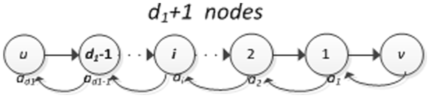Then, the time for the message to reach node 2 is $⌈ (a_{1} + 2) / Q ⌉ * S$ . Easily, we can get $a_{2} = a_{1} + ⌈ (a_{1} + 2) / Q ⌉ * S$ . Similarly, we can get that $a_{i} = a_{i - 1} + ⌈ (a_{i - 1} + i) / Q ⌉ * S$ . The lemma holds.

Figure 2.

A journey between u and v.

Lemma 2 and Lemma 3 provide basis to calculate time delay of messages, for neighboring node pairs and non-neighboring node pairs, respectively. Such calculation is necessary for distributed algorithms, including counting algorithms, to control message transfer and communication operations according to time.

Relationship between (Q, S)-distance and (Q, S)*-distance

The two dynamicity models defined above are related with each other. (Q, S)-distance model describes the distance change of any pair of nodes, while the (Q, S)*-distance model defines distance change of neighboring nodes. Intuitively, (Q, S)-distance is more general than (Q, S)*-distance, in terms of the scenarios considered, that is, one-hop journey or multi-hop journey.

However, it is more interesting to consider their relationship in terms of their power in distributed computing. Which model is more powerful in providing dynamicity properties desired in distributed algorithms? Does a dynamic network defined by the (Q, S)*-distance model also satisfy the definition of (Q, S)-distance? After carefully examining the properties defined in the two models, we get two interesting conclusions.

(Q, S)-distance and (Q, S)*-distance are equivalent

First, we consider the power of defining distance dynamicity. We find out that these two models are equivalent. That is, a network with (Q, S)-distance can be always defined by a (Q, S)*-distance model and vice versa. This is a very interesting conclusion and we prove it as below.

Lemma 4

If a dynamic network follows the (Q, S)*-distance model, it also follows the (Q, S′)-distance model, where S′ is (n − 1)*S and n is the total number of nodes in the network.

Proof

For any node u and v, the dynamic distance between them is d_u,t(v) at time t. Then, a message from u needs to be forwarded by at most d_u,t(v) nodes (including u) to reach v. As shown in Figure 2, each pair of nodes i and i − 1 are neighbors of each other when node i forwards the message from u to v. By Definition 6, if the network follows (Q, S)*-distance model, the dynamic distance between i and i − 1 is at most $1 + ⌈ (t' - t) / Q ⌉$ at some time t′, that is, $d_{i - 1, t'} (i) \leq 1 + ⌈ (t' - t) / Q ⌉$ . Then

d_{v, t'} (u) \leq \sum_{i = 1}^{d_{u, t} (v)} d_{i - 1, t'} (i) \leq d_{u, t} (v) + ⌈ (t' - t) / Q ⌉ * d_{u, t} (v) * S

Since the dynamic network is 1-interval connected, the dynamic distance between any two nodes is at most n 1, that is, d_{u, t}(v) ≤ n 1. Then, we can get $d_{v, t'} (u) \leq d_{u, t} (v) + ⌈ (t' - t) / Q ⌉ * (n - 1) * S$ . By Definition 6, the dynamic network follows the (Q, (n − 1)*S)-distance model. The lemma holds.

Lemma 5

If a dynamic network follows a (Q, S)-distance model, it also follows a (Q, S)*-distance model.

Proof

By Definition 4 and Definition 6, d_u,_t(v) = 1 in (Q, S)*-distance model is an especial case of d_u,t(v) in (Q, S)-distance model. Then, a dynamic network follows a (Q, S)-distance model also follows the (Q, S)*-distance model. The lemma holds.

Theorem 4

The (Q, S)*-distance model and (Q, S)-distance model are equivalent in terms of the power of describing distance changes.

Proof

By Lemma 4 and Lemma 5, the theorem obviously holds.

(Q, S)*-distance is more accurate

The second conclusion is about accuracy. By Lemma 5, a (Q, S)-distance model can be converted to a (Q, S)*-distance model, with the same value of S. However, by Lemma 4, a (Q, S)*-distance model can only be converted to a (Q, (n − 1)*S)-distance model, where (n − 1)*S is obviously larger than S. In terms of accuracy of distance calculation, (Q, S)*-distance is better than (Q, S)-distance. Thus, we use different names for these two models.

Then, given a specific network, we can always find a (Q, S)*-distance model with a S not greater than the corresponding (Q, S)-distance model. Namely, (Q, S)*-distance is better than (Q, S)-distance. Such advantage in accuracy can help upper algorithms conduct operations with fewer rounds and reduce both time cost and message cost.

Algorithm 1—the basic algorithm for counting in a flat network

Based on (Q, S)-distance model, we design the first diffusing computation algorithm for counting. Different from typical diffusing computation, this algorithm contains three phases.

The first phase is still the growing phase, which is used mainly for constructing the tree structure. The third phase is the shrinking phase, which is used to collect information from the network. For the counting problem, the information collected is simply the number of children. These two phases are similar to but not the same as those in typical diffusing computation, because new operations are necessary to handle topology changes. More importantly, a totally new phase, called notifying phase, is added between the growing phase and the shrinking phase. This phase serves the purpose of determining the termination of growing phase and invoking the shrinking phase.

As pointed out in section “Diffusing computation and its problems in dynamic networks,” topology changes bring two challenges in diffusing computation: how to determine the leaf nodes and terminate growing and when to stop sending a message between children and parent when the neighborhood is destroyed. To help understanding our algorithm and the novelty, we describe the basic ideas of addressing these two challenges as below.

To avoid missing of moving nodes, all nodes in active keep broadcasting the initiation message. Then, key point is when to stop such broadcasting and switch to shrinking. In our algorithm, we let the initiator take the job of detecting termination of growing. More precisely, during the growing phase, in every Qth+1 round, the nodes that receive their first initiation message in the Qth round will send a signal message to the initiator, where Q is the value in the (Q, S)-distance model. Based on the (Q, S)-distance model, the initiator node can calculate the upper bound on the arrival time of signal messages and consequently determine whether all the nodes have joined the tree. Then, the initiator will invoke the notifying phase to notify others about the termination of growing phase. The notification message will be disseminated along the diffusing tree established in the growing phase. Upon receiving notification from initiator, each node will switch to shrinking phase and determine whether it is a leaf node. The first challenge is addressed.

When a message is sent between a child and its parent, the sender will keep sending it round by round and the intermediate nodes will keep forwarding it. Since the communication is in synchronous rounds, based on the (Q, S)-distance model, the sender can calculate the upper bound on the dynamic distance between the child and parent, and this distance can be used to set the number of rounds for sending and forwarding the message. The second challenge is addressed.

In the following, we first describe the detailed operations of our algorithm and then prove its correctness together with the results of performance in time cost and message cost. Finally, we discuss about variant operations to improve the algorithm.

Detailed operations of Algorithm 1

In our algorithm, for the simplicity of presentation, we use “black” and “white” to refer to active node and inactive nodes, respectively. Then, the procedure of tree growing is in fact the procedure of coloring nodes from white to black (Figure 3).

Figure 3.

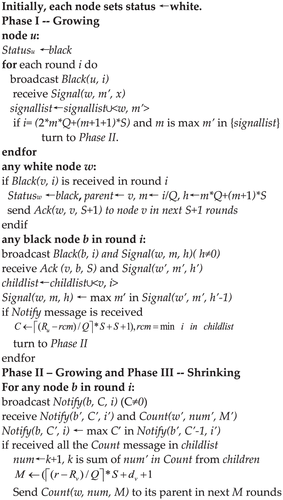
The pseudocode of Algorithm 1.

Phase I—growing

Initially, each node is white. When the initiator node u wants to do counting, it invokes the algorithm by coloring itself to be black and broadcasts the initiation message Black(u, r), where r is the round number and is set to be one by u. Then, the tree is established by the diffusing of Black messages, round by round. Notice that the initiator is any node, which wants to get the number of nodes in the network.

Upon receiving a black message Black(v, r), a white node w joins the tree by coloring itself to be black, and v will be accepted as its parent. Then, in the next round and later rounds, node w broadcasts the black message Black(w, r + 1) to its neighbors.

Moreover, node w needs to send two other messages. One is Ack(w, v, S+1) to its parent v to let v add w to its child list, where S is the value in (Q, S)-distance model. If r is the integral multiple of Q, node w will also need to send the other message Signal(w, m, H) to the initiator u, where m = r/Q, and H = m*Q+(m+1)*S. To cope with topology changes, w will keep broadcasting the Ack message in the following S+1 rounds and the signal message in the following H rounds.

Please notice that the limit of rounds for sending and forwarding can be realized by decrementing the limit counter, for example, H in Signal message, by one at each forwarding. Moreover, although three types of messages may need to be sent by node w in one round, they can be merged together and sent in one broadcast as one single message.

When node x receives the Ack message originated from w, it records <w, rc> in its child list, where rc is the current round number. Then, the child-parent relationship between w and x is established.

When node u receives the signal message Signal(w, m, x), it records <w, m> in the signal list. Then, it will expect the next Signal message that should arrive in or before the round (2*m*Q+(m+1+1)*S). If such a message does not arrive in or before the expected round, u will switch to the second phase. Please notice that, due to topology dynamicity, the series of Signal message may not be delivered in the order of sending, but this does not matter, because a Signal message received by u earlier than expected is obviously viewed as arriving in time.

Phase II—notifying

Phase II is started with sending notification message by node u. Node u sends Notify(u, C_u, r) to its children, where C_u is the limit of rounds that the message should be sent and forwarded and r is the current round number. With (Q, S)-distance model, C_u is set to be $(⌈ (R_{u} - rcm) / Q ⌉ * S + S + 1)$ , where rcm is the minimum of the round numbers of receiving Ack messages from children.

When the node w receives Notify(v, C_v, R_v) from its parent v, it will stop broadcasting Black message and sends Notify(w, C_w, r) to its own children, where r is the current round. Node w records <R_v, d_v> in its parent list, where d_v = r − R_v and r is the current round number. If w does not have children, that is, it is a leaf node, it will switch to Phase III.

Phase III—shrinking

Phase III starts with sending Count messages at leaf nodes. A leaf node w sends Count(w, num, M) to its parent node v, where num is the number of children plus one. This message will be sent and forwarded in the following M rounds, with $M = (⌈ (r - R_{v}) / Q ⌉ * S + d_{v} + 1$ .

For a non-leaf node v, if it has received a Count message from each child, it will construct its own count message Count(v, num, M) to its parent, where num is the sum of all the count values from children plus one.

Finally, the initiator node u will receive the Count message from all its children and can calculate the final count results by sum the count values from them. Phase III ends.

Correctness and performance

To prove that Algorithm 1 solves the counting problem defined in Definition 2, we need to prove it has the termination property and accuracy property.

Lemma 6

Before Phase II starts at the initiator node, if there exist any white nodes in the end of some round r′, then at least one white node will be colored to black in round r′+1.

Proof

Since the network is 1-interval connected, at least one white node, say x, has a neighbor in black at the beginning of some round r′+1. Because Notify message has not yet been sent out by the initiator, the black neighbor of x must broadcast Black message in r′+1 and x will receive the Black message and join the tree by coloring itself to be black in round r′+1. The lemma holds.

Lemma 7

At the end of Phase I, the diffusing tree structure contains all nodes in the network, and each node knows its parent and children.

Proof

The proof of the first part is by contradiction. Assume that one or more nodes are still white at the moment that the initiator node u starts notifying phase in round q.

Without loss of generality, we assume the initiator u switches from Phase I to Phase II due to the miss of the Signal message m′, which should be received by u in or before the round (2*m′*Q+(m′+ 1)*S). Then, q = (2*m′*Q+(m′+ 1)*S)+1.

By Lemma 1, a message Signal(w, m, H) can be delivered to node u in most m*Q+(m+1)*S rounds. Missing the Signal message indicates that no white node turns black in round m′*Q, which contradicts with Lemma 6. Obviously, the first part holds.

The second part is easier to prove. Since each node accepts the sender of the first received Black message as its parent, a child obviously knows about its parent. A parent gets to know about its child via Ack message. Due to topology changes, An Ack message may be sent to the parent node via multi-hop journey. By Lemma 1, an Ack message Ack(w, v) can be delivered in at most S+1 rounds. Lemma 7 holds.

Theorem 2 (termination)

Algorithm 1 can terminate in O(D²) rounds, where D is upper bound of the network dynamic diameter, and the message size is Θ(clogn) in general cases and Θ(nlogn) in the worst case, where c is equal to $2^{(⌈ (R_{u} - rcm) / Q ⌉ * S + S + 1)}$ .

Proof

The duration of Phase I is determined by the diffusing time of Black message. Since Black message is propagated via direction connect between neighbors, Phase I can be completed in O(D) rounds. Please notice that, although Ack messages and Signal messages may be delivered via multi-hop journey, they are in fact carried by Black messages and do not affect the overall end time of Phase I.

In Phase II and Phase III, all the connection between children and parents may be multi-hop. Since each message can be delivered in at most D rounds, and the depth of the tree structure is at most D, Phase II and Phase III can be completed terminate in at most O(D²) rounds.

The message size of each message type is determined by the information carried. In general cases, node ID, number of nodes and tree depth are all in the same order of network size n, and can be represented using Θ(logn) bits, the message size of algorithm is in the size of Θ(logn) bits.

In the worst case, when the notification message send by node u is received by all nodes, the message size of algorithm is Θ(n) bits.

Since the Notify message is forwarded by $(⌈ (R_{u} - rcm) / Q ⌉ * S + S + 1)$ rounds, then in general cases, a node needs to send at most $2^{(⌈ (R_{u} - rcm) / Q ⌉ * S + S + 1)}$ Notify messages in one round, and the message size is $Θ (2^{(⌈ (R_{u} - rcm) / Q ⌉ * S + S + 1)} logn)$ bits. In the worst case, that is, $(⌈ (R_{u} - rcm) / Q ⌉ * S + S)$ is greater than D, some nodes need to send all Notify messages in one round, and the message size is Θ(nlogn) bits. The theorem holds.

Theorem 3 (accuracy)

At the end of phase III, node u can get the accurate number of nodes in the network.

Proof

By Lemma 1, we can easily get that, for each node, it can surely receive Notify(ID, C_ID) from its parent, and Count(ID, num, M) from all its children. By Lemma 7, all the nodes are included in the diffusing tree, so node u can get the accurate number of nodes after it receives Count message from each child. The Theorem holds.

Variant operations

Algorithm 1 described above can be improved by the following points.

Intermediate notification

In Phase II of Algorithm 1, the Notify message is sent from a parent to children and the Notify message may be forwarded by intermediate nodes. It is possible that an intermediate node has not received Notify message from its parent. Then, such a node can switch to Phase II upon the Notify forwarded and does not need to wait for the Notify message from its parent. This can obviously speed up the execution of Phase II and Phase III.

Under T-interval connectivity

In Algorithm 1, we assume 1-interval connectivity, which is quite weak in terms of topology stability. It can reduce message cost under T-interval connectivity,¹² which stipulates that, for every T consecutive rounds, there exists a stable connected spanning subgraph.

If the network is T-interval connected, the nodes do not need broadcasting Black messages in each round. Instead, each node needs to broadcast Black message once per T rounds. It is similar for other messages.

From (Q, S)-distance to (Q, S)*-distance

The algorithm described above is originally designed based on the (Q, S)-distance model. As discussed in section “The (Q, S)-distance model and (Q, S)*-distance model,” the (Q, S)*-distance model is more accurate. To adapt the algorithm to (Q, S)*-distance model, the following modifications need to be done.

In Phase I, a node u needs to calculate the upper bound of the arrival round of Signal(w, m, x) based on Lemma 3. With (Q, S)-distance model, the bound is (2*m*Q+(m+1+1)*S). If (Q, S)*-distance model is assumed, the bound will be a_m_*s, where $a_{i} = a_{i - 1} + ⌈ (a_{i - 1} + i) / Q ⌉ * S$ , and a₁ = S.

The other messages exchange in Algorithm 1 are between parents and children (more precisely the ending nodes have ever been neighbors of each other), the calculation of distance difference can be the same except that the value S needs to be replaced with the new value in the (Q, S)*-distance model.

Algorithm 2—the improved algorithm for counting in a flat network

Algorithm 2 is an improvement of Algorithm 1, by removing the Signal message so as to save message cost. In Algorithm 1, when a node turns black in round r and r is an integral multiple of Q, it will send a Signal(w, m, H) message to the initiator node. The Signal message is used by the initiator node to determine whether all nodes in the network have joined the tree, that is, all the nodes have turned to be black.

After carefully considering the information carried with a Signal message, we find that essential information needed by the initiator is the maximum round when a node turns to be black. Then, we can remove the Signal message and manage to send back the round number of turning black. More interesting, such information can be piggybacked on the Black message. Compared with the operations in Algorithm 1, such a design can save message cost. Moreover, the round number of turning black can also help the initiator terminate Phase I earlier and consequently save overall execution cost. Such advantages will be analyzed in the end of this section.

Same as Algorithm 1, Algorithm 2 is described below using the (Q, S)-distance model, and it can be adapted to the (Q, S)*-distance model similarly as Algorithm 1.

Detailed operations of Algorithm 2

Similar to Algorithm 1, Algorithm 2 also contains three phases. The major difference lies in the operations in Phase I, that is, no Signal messages, new Black messages and new termination condition of Phase I.

Initially, each node is white. When the initiator node u wants to do counting, it invokes the algorithm by coloring itself to be black and broadcasting the initiation message Black(u, r = 1, m = 1), where r is the number of the current round and m is the round number that the node turns black. Then, the tree is established by the diffusing of Black messages, round by round.

Upon receiving a black message Black(v, r, m), a white node w joins the tree by coloring itself to be black, and v will be accepted as its parent. Then, in the next round, node w broadcasts the black message Black(w, r+1, r+1) to its neighbors. In the later rounds, node w broadcasts message Black(w, r′, M), where r′ is the number of the current round and M is the maximum of the values of “m” carried with Black messages received by w.

The operations on Ack messages are similar to those in Algorithm 1. Node w sends Ack(w, v, S+1) to its parent v to let v add w to its child list, where S is the value in (Q, S)-distance model. To cope with topology changes, w will keep broadcasting the Ack message in the following S+1 rounds. When node x receives the Ack message originated from w, it records <w, rc> in its child list, where rc is the current round number. Then, the child-parent relationship between w and x is established.

The handling of Black message at the initiator node is different from that in Algorithm 1. When node u receives the message Black(u, r, m), it will update the value of M kept for the maximum “m.” Then, node u will expect that a message Black(u, r, m) with m > M will arrive in or before the round $m + 1 + ⌈ (m + 1) / Q ⌉ * S$ . If such a message does not arrive in or before the expected round, u will terminate Phase I and switch to the second phase.

The operations of the other two phases are almost the same as those in Algorithm 1. Here, we do not repeat them.

Correctness proof

Lemma 8

For any m carried with a message Black(u, r, m), the initiator node u either receives the m or receives some value m′ that is greater than m, in or before the round $m + 1 + ⌈ (m + 1) / Q ⌉ * S$ .

Proof

By Lemma 1, when node w turns black in round m, there exists a journey along which the message Black(v, r, m) can reach node u in or before the round $m + 1 + ⌈ (m + 1) / Q ⌉ * S$ . According to the operations in Phase I, any black node v will broadcast message Black(v, r, M), where M is the maximum of the values of “m” carried with Black messages received by v. If node u does not receive message Black(v, r, m) in or before the round $m + 1 + ⌈ (m + 1) / Q ⌉ * S$ , the value m must have been replaced with another greater value at some node along the journey. The lemma holds.

Lemma 9

At the end of Phase I, the diffusing tree structure contains all nodes in the network, and each node knows its parent and children.

Proof

For By Lemma 8, if some nodes turn into black in round m, node u will receive m′ which is not smaller than m in or before the round $m + 1 + ⌈ (m + 1) / Q ⌉ * S$ . If such a message does not arrive in or before the expected round, it means that no nodes turns to black in round m. Since the network is 1-interval connected, at least one white node will turn black in round m until all the white node turn black. Thus, the diffusing tree structure contains all nodes in the network. The lemma holds.

Theorem 4 (termination)

Algorithm 2 can terminate in O(D²) rounds, where D is upper bound of the network dynamic diameter, and the message size is Θ(clogn) in general cases and Θ(nlogn) in the worst case, where c is equal to $2^{(⌈ (R_{u} - rcm) / Q ⌉ * S + S + 1)}$ .

Proof

The duration of Phase I is determined by the diffusing time of Black message. Since Black message is propagated via direction connect between neighbors, Phase I can be completed in O(D) rounds. Differ to Algorithm 1, Signal message has been removed in Algorithm 2. Thus, the message size in Algorithm 2 is smaller than in Algorithm 1.

The operations of the other two phases are almost the same as those in Algorithm 1. Thus, the cost of Phase II and Phase III in Algorithm 2 is the same as Algorithm 2. By Theorem 2, we can get that Algorithm 2 can terminate in O(D²) round, and the message size is Θ(clogn) in general cases and Θ(nlogn) in the worst case, where c is equal to $2^{(⌈ (R_{u} - rcm) / Q ⌉ * S + S + 1)}$ . The theorem holds.

Comparison with Algorithm 1

Compared with the operations in Algorithm 1, Algorithm 2 can save both message cost and time cost. In Algorithm 1, Signal messages are sent with an interval of Q rounds and forwarded by intermediate nodes, removing Signal in Algorithm 2 will save message cost.

Moreover, Algorithm 1 determines the time to terminate Phase I based on the Signal message and the message is sent with an interval of Q rounds, so the initiator cannot know the exact round that the last node joins the diffusing tree. In Algorithm 2, by the maximum round number carried in Black message, Algorithm 2 can terminate Phase I accurately and earlier than Algorithm 1, and both time and messages can be saved.

Algorithm 3—the algorithm for counting in a hierarchical network

Cluster-based hierarchy is very popular in ad hoc networks to reduce communication cost and improve topology control efficiency. In our previous work,²² we have considered cluster-based hierarchy in dynamic networks and designed hierarchical algorithms for information dissemination.

In this section, we discuss how to extend our flat counting algorithms to hierarchical ones. Since the extension to Algorithm 1 and Algorithm 2 are similar, we present the hierarchical design for only Algorithm 1 and name the new algorithm “Algorithm 3.”

To make use of cluster hierarchy in dynamic networks, additional models and assumptions on the stability and connectivity are obviously necessary. In the design of Algorithm 3, we propose the (Q, S)-distance clusterhead model, which is defined based on our recent work on information dissemination.²²

In the following, we first present necessary models and assumptions used and then describe the operations of Algorithm 3. Finally, we prove its correctness and analyze its performance. We also compare the two algorithms in terms of both time cost and communication cost.

The (Q, S)-distance clusterhead model

In a dynamic network with cluster hierarchy, all the network nodes are grouped into clusters, each of which is coordinated by a clusterhead node, as illustrated in Figure 4. A clusterhead is in charge of forwarding messages from/to its cluster members. We assume cluster member and clusterhead is connected via direct connection, that is, one-hop broadcasting. The cluster hierarchy may change from time to time due to topology changes, for example, a node may switch from one cluster to another, according to the clustering mechanism. We assume that each switch is completed within one round. Clusterhead and cluster members know each other via the clustering mechanism.

Figure 4.

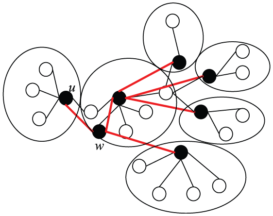
A hierarchical dynamic network.

To model such a dynamic network with cluster-based hierarchy, the dynamic graph described in section “System model and problem definition” is extend to a hierarchical dynamic graph:²²G′ = (V, E, Γ, ζ, C, I), where V is the set of nodes in the network, E is the edge matrix, Γ is lifetime of the system in terms of synchronous communication rounds, ρ is the presence function indicating whether a given edge is available at a given time, and ζ is the latency function representing the time taken to cross an edge. C: V × Γ → {h, g, m} is the status of each node at a given time, with h indicates clusterhead, g indicates that the node is a cluster gateway node, which is responsible for forwarding packets between clusters, and m indicates that this node is a common node, that is, a cluster member.

Definition 7 (T-interval clusterhead connectivity)

We say that a dynamic network has T-interval clusterhead connectivity if: $\forall i \in N, \exists ϒ \subseteq G_{i} : V_{ϒ} \supseteq V_{h}^{i}$ , $ϒ$ is connected subgraph, and $\forall j \in [i, i + T - 1), ϒ \subseteq G_{j}$ .²²

Please notice: $V_{h}^{i}$ : is the set of clusterhead nodes in the time.

Definition 8 (L-hop clusterhead connectivity)

We say that the connectivity among clusterheads is L-hop if: $\min {L | \forall S \subset V_{h}^{i}, v \in V_{h}^{i} \ S$ , and $\exists u \in S$ , distance(u, v) ≤ L}.²²

In fact, L indicates the maximum value of the shortest path between any two clusterheads that connected directly or by only gateway nodes.

Definition 9 (T-interval L-hop clusterhead connectivity)

The cluster-based hierarchy with both T-interval clusterhead connectivity and L-hop clusterhead connectivity in the subgraph $ϒ$ .²²

To design hierarchical counting algorithm, we define the (Q, S)-distance clusterhead model, which defines the change of dynamic distance among the clusterhead nodes by simply extending (Q, S)-distance.

Definition 10 ((Q, S)-distance clusterhead)

We say that a cluster-based hierarchy is connectivity with (Q, S)-distance among clusterheads that

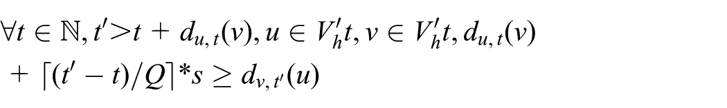
\forall t \in ℕ, t' > t + d_{u, t} (v), u \in V_{h}^{'} t, v \in V_{h}^{'} t, d_{u, t} (v) + ⌈ (t' - t) / Q ⌉ * s \geq d_{v, t'} (u)

where $V'_{h}^{t} = ⋃_{0}^{t} V_{h}^{t}$ .

Detailed operations of Algorithm 3

In our design, we assume that the cluster hierarchy is established by underlying clustering algorithm, which is out the scope of our work. Since the cluster hierarchy model is based on T-interval connectivity, Algorithm 3 also assumes T-interval connectivity. The cluster hierarchy should be with T-interval L-hop Clusterhead Connectivity and (Q, S)-distance clusterhead.

Algorithm 3 extends Algorithm 1 by incorporating the cluster hierarchy, and it also contains three phases. The major difference between Algorithm 3 and Algorithm 1 is that we try to construct the diffusing tree among clusterhead nodes rather than all the nodes. That is, only clusterhead nodes are really participating in the diffusing operations. Common members only need to let some clusterhead count it in the results. Obviously, such a design will significantly reduce the communication cost of counting.

The major challenge in the design of cluster-based counting algorithm lies in the dynamicity of cluster membership. More precisely, a member node may be missed due to cluster switches. We address this by making use of the three-phase design to obtain a consistent cluster membership among all clusters.

Phase I—growing

As in Algorithm 1, every node is white initially, and the counting algorithm is triggered by the initiator node u. Without loss of generality, we assume u is a clusterhead node. It first colors itself to be black and then broadcasts the initiation message Black(u, r), where r is the round number and is set to be one by u. Then, the tree is constructed by diffusing Black messages. Each black node broadcasts the Black message in the every Tth+1 round.

When a white gateway node receives a black message Black(v, l), if this is the first Black message received in the current period of T rounds, it broadcasts Black(v, l+1) to its neighbors. Please notice that a gateway node will not change its color here.

When a white clusterhead node w receives a black message Black(v, l) in round r, it joins the tree by coloring itself to be black, and v will be accepted as its parent. Node w sets B_w, the round number it turns black, to be r.

From this round r, clusterhead node w needs to record the number of its cluster members for each round until it gets the Notify message. This operation is important, because one of such numbers will be used as the count of w’s cluster and included in the final counting result.

In the next round r+1, node w broadcasts the message Black(w, r+1) to its neighbors. Moreover, same as in Algorithm 1, node w needs to send two other messages. One is Ack(w, v, S + L, B_w) to the parent v to inform about the new child. S is the value in (Q, S)-distance model, and L is the value in T-interval L-hop clusterhead connectivity. If $⌈ r / T ⌉ * T - r \leq L - 1$ , node w will also need to send the other message Signal(w, m, H) to the initiator u, where $m = ⌈ r / T ⌉$ and $H = m * T + ⌈ (m * T + 1) / Q ⌉ * S$ . Same as in Algorithm 1, to cope with topology changes, w will keep broadcasting the Ack message in the following S + L rounds and the Signal message in the following H rounds. These three messages can be in fact merged into integrated one.

When a clusterhead x receives the Ack message originated from w, it records <w, rc, B_w> in its child list, where rc is the current round number. When the initiator u receives the signal message Signal(w, m, x), it records <w, m> in the signal list.

Same as in Algorithm 1, when some Signal message m′ does not arrive in or before the round, Phase I finishes and u will invoke the second phase.

Phase II—notifying

Phase II is triggered by the missing of Signal message m′ at u. To collect consistent count values in spite of cluster membership changes, the initiator appoints the clusterheads to count the number of members it had in the specific round F, where F = m′*T. Such a value is chosen because it is a round that all clusterheads have become black and recorded their number of members. The detailed discussion is shown in correctness proof.

Node u starts Phase II by sending the notification message Notify(u, C_u, R_u, F) to its children, where C_u is the limit of rounds that the message should be sent and forwarded, and R_u is the current round number. With the (Q, S)-distance clusterhead model, C_u is set to be $(⌈ (R_{u} - rcm) / Q ⌉ * S + S + 1)$ , where rcm is the minimum of the round numbers of receiving Ack messages from children.

When a clusterhead w receives Notify(v, C_v, R_v, F), it will stop broadcasting Black message and also stop recording the number of its cluster members. It also sends Notify(w, C_w,, R_w, F) to its own children in the diffusing tree. Node w records <R_v, d_v> in its parent list, where d_v = r − R_v and r is the current round number. If w does not have children, that is, B_ID ≤ F, it is a leaf node and will switch to Phase III.

Phase III—shrinking

Phase III starts with sending Count messages by leaf nodes, that is, the clusterheads with no children turning black before F. Node w sends Count(w, num, M) to its parent node v, where num is the number of its cluster members in round F. This message will be sent and forwarded in the following M rounds, with $M = (⌈ (r - P_{v}) / Q ⌉ * S + d_{v} + 1)$ .

The following procedure of shrinking among clusterheads is almost the same as that in Algorithm 1, except that only clusterheads generate and aggregate node numbers as tree nodes, and only the cluster members in the specific round F are counted.

Please notice that if clusterhead node was not acting as a clusterhead in round F, it is viewed as a clusterhead with no members (even not itself).

Finally, the initiator node u will receive the Count message from all its children and can calculate the final count results by sum the count values from them plus the number of its cluster in round F. Phase III ends.

Correctness and performance

Lemma 10

With Algorithm 3, at the end of Phase I, the diffusing tree structure contains all clusterheads in the round F, and each clusterhead knows its parent and children.

Proof

The proof of the first part is by contradiction. Assume one or more clusterhead nodes are still white in round m′*T.

Since the network is T-interval L-hop clusterhead connected, at least one white clusterhead turns to black in per L rounds until all the clusterhead turns to black. Therefore, at least one white clusterhead turns to black between round m′*T − L and m′*T.

By Lemma 1, a Signal(w, m, H) can be delivered to node u at most $m * T + ⌈ (m * T + 1) / Q ⌉ * S$ rounds. Node u has not received m′ in Signal message in round $m' * T + ⌈ (m' * T + 1) / Q ⌉ * S$ , that means no white node turns black between round m′*T − L and m′*T. This contradicts with “at least one white clusterhead turns to black between round m′*T − L and m′*T.

The second part is proved as follows. Since each node accepts the sender of the first received Black message as its parent, a child obviously know about its parent. A parent gets to know about its child via Ack message. Due to topology changes, an Ack message may be sent to the parent node via multi-hop journey. By Lemma 1, an Ack message Ack(w, v) can be delivered in at most S + L rounds.

Based on the proof of two parts, the lemma holds.

Theorem 5 (termination)

Algorithm 3 can terminate in O(D²) rounds, where D is upper bound of diameter of networks, and the message size is Θ(clogn) in general cases and Θ(n₀logn₀) in the worst case, where c is equal to $2^{(⌈ (R_{u} - rcm) / Q ⌉ * S + S + 1)}$ and n₀ is the upper bound on the number of clusterhead nodes.

Proof

The proof is similar to that of Theorem 2 and omitted here.

Theorem 6 (accuracy)

At the end of phase III, node u can get the accurate number of nodes in the network.

Proof

By Lemma 1, we can easily get that, for each node, it can surely receive Notify(u, C_ID, R_ID, F) from its parent, and Count(ID, num, M) from all its children which B_ID is not greater than F. By Lemma 10, all the clusterheads in round m′*T are included in the diffusing tree, so node u can get the accurate number of nodes after it receives Count message from each child. The Theorem holds.

Performance comparison with Algorithm 1

It is interesting to compare the performance of our both algorithms. First, we consider time cost. As proved in Theorem 2 and Theorem 4, the time complexity of both our counting algorithms is in O(D²) of rounds. In fact, the exact time cost of the counting algorithms is determined by not only the diameter of the network but also the number of nodes participated. Since Algorithm 3 has fewer nodes really participating than Algorithm 1, Algorithm should be able to terminate earlier than Algorithm 3, although the exact difference is hard to analyze.

The difference in communication cost is more obvious and easier to analyze. Roughly, we evaluate communication cost using the total bits broadcasted (or transmitted) by all the nodes, which is roughly determined by three factors: the execution time, that is, time cost in rounds, message size, and the number of nodes participated.

For Algorithm 1, by Theorem 2, we can get that Phase 1 has the communication cost is in O(D²*n²*logn) bits. The communication cost of Algorithm 3 is calculated based on the number of clusterhead, rather than total number of nodes (the cost at gateway nodes can be neglected in such rough analysis).

By Theorem 5, we have the communication cost of Algorithm 3 in O(D²* $n_{0}^{2}$ *logn) bits, where n₀ is the upper bound on the number of clusterhead nodes and gateway nodes in m′*T rounds. Considering that n₀ is usually much smaller than n, the communication cost of Algorithm 3 is much less than that of Algorithm 1.

Simulation results

To the best of our knowledge, existing algorithms are not suitable for (Q, S)-distance model. Thus, we do not simulate existing counting algorithms, that is, the simulation cannot be used to compare with existing algorithms. The simulation is used to validate the correctness of our algorithms and measure their performance quantitatively. We conduct simulations via a widely used simulator, ns-3.

Simulations setup

We simulate a network with wireless ad hoc nodes randomly distributed in a 1000 m × 1000 m area. The range of communication radio is set to be 100 m. The speed of node movement is set to be 20 m per round. One round is simulated by one send–receive period.

To “realize” the assumptions on dynamicity defined in our (Q, S)-distance model, we vary the period of send-receive round and then different (Q, S) values are achieved.

The performance of a counting algorithm is measured via three metrics: accuracy, time cost, and message cost. Accuracy refers to how accurate the number of nodes counted against the real number of nodes. Counting time is defined as the number of rounds used to compete counting. Message cost refers to the average number of messages sent by one node.

Simulation results

We first examine the effect of (Q, S) values. For ease of simulating, we fix the movement speed of nodes(S = 5) and change Q values by controlling the time duration of each send-receive round. Then, we examine the effect of network size, that is, the number of nodes N.

Accuracy

The results of accuracy are plotted in Figure 5. All our algorithms can achieve accurate counting results. This is expected and such results confirm our correctness proof in previous sections.

Figure 5.

Accuracy of counting: (a) accuracy versus Q, with S = 5, N = 160 and (b) accuracy versus N, with S = 5, Q = 6.

Time cost

The results of time cost in terms of number of rounds used to complete counting are shown in Figure 6. Roughly, our algorithms need 100 to 150 rounds to complete the counting task in various cases. Among the three algorithms, the cluster-based algorithm can always outperform the other two. This clearly indicates the benefit of cluster hierarchy. Algorithm 2 needs fewer rounds due to the mechanism to terminate Phase I earlier than Algorithm 1.

Figure 6.

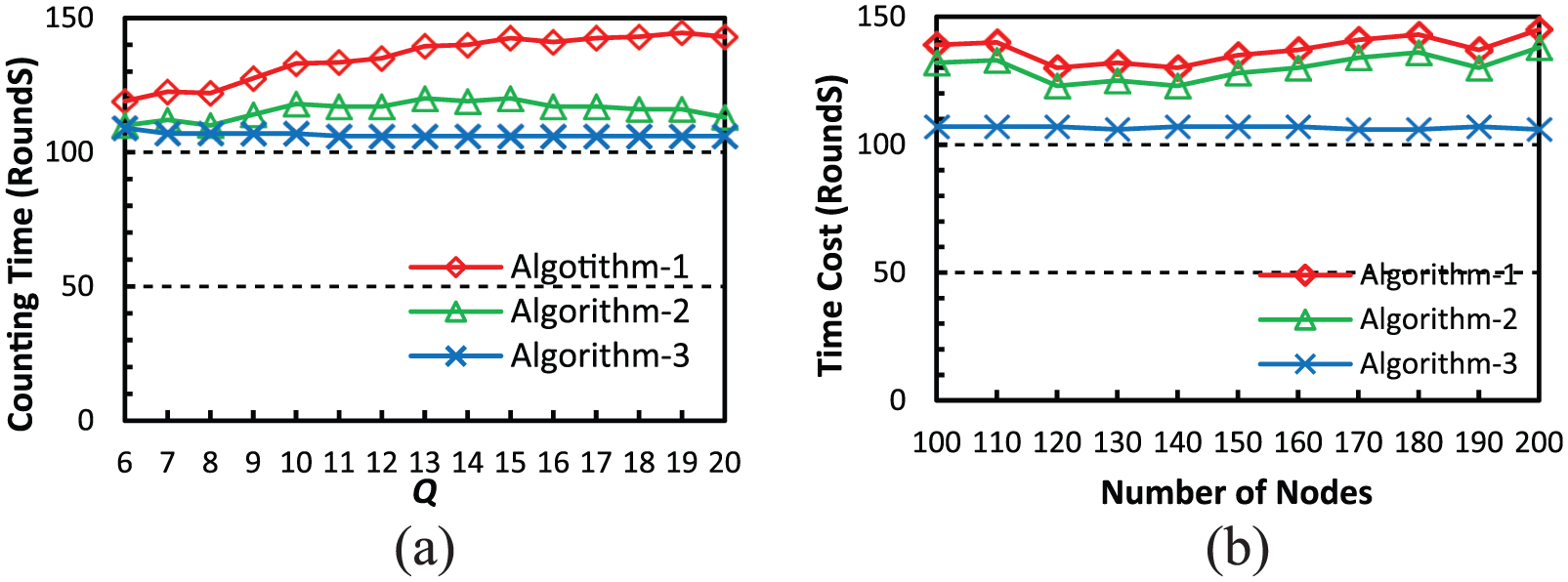
Time cost: (a) time cost versus Q, with S = 5, N = 160 and (b) time cost versus N, with S = 5, Q = 6.

Figure 6(a) also shows that the change of Q-value or number of nodes affects time cost significantly, except that of Algorithm 3. Intuitively, when S is fixed, a larger Q value means less dynamicity and counting should be completed with fewer rounds. However, Figure 6 shows that a larger Q results in more rounds for counting, especially in Algorithm 1. Such an interesting effect may be explained by the change of “dynamic diameter.” On one hand, link breakage due to node movement may cause the increase of diameter. On the other hand, link establishment may cause decrease of diameter. Therefore, under the accumulative effect of such two aspects, high dynamicity may cause longer or shorter counting time.

The effect of network size is shown in Figure 6(b). Roughly, more nodes in the system will cost more rounds to count them. Benefiting from the cluster hierarchy, Algorithm 3 is not affected much by the change of network size.

Message cost

The results of message cost, in terms of the average number of messages sent at one node, are shown in Figure 7. The change of Q value does not affect message cost much, in all three algorithms. However, network size is a dominating factor in message cost. This is expected. More nodes in the system, more neighbors may present and then more messages are exchanged for counting. However, Algorithm 3 is not affected much by N, which shows that cluster hierarchy is a good choice to improve scalability.

Figure 7.

Message cost: (a) message cost versus Q, with S = 5, N = 160 and (b) message versus N, with S = 5, Q = 6.

Conclusion and future work

In this article, we study the distributed counting problem in the environment of dynamic networks. The major challenge lies in the dynamicity caused by topology changes. Based on the notion of dynamic distance, we propose two system models, called (Q, S)-distance and (Q, S)*-distance, which are defined to describe the change of distance between a pair of nodes. Based on these models, we design three dynamic counting algorithms. We basically adopt the classical approach of diffusing computation and design mechanisms to handling dynamic topology changes. The three algorithms differ in mechanisms to determining growing phase and network architecture, and consequently, they have different message costs and time costs. Compared with existing counting algorithms, our algorithms can terminate deterministically with accurate results.

Since counting in dynamic networks is a fundamental but challenging problem in distributed computing, much more efforts are obviously necessary. One interesting direction is new dynamicity models in terms of node mobility, rather than “dynamic distance.” Mobility model is a more direct view of network dynamicity, but it is more difficult to be adopted in theoretical algorithm design for distributed computation problems like counting. Other possible directions include counting in asynchronous network, more general cluster hierarchy with multi-hop clusters, and so on.

Footnotes

Acknowledgements

This manuscript is an extension of our conference paper published in the proceedings of SRDS’14.⁴ In the extend version, we have added quite a lot of new and significant content to make our work more solid and significant. We have defined a new dynamic model and discussed the relationship between two modes, which make our work more general. We have designed a new algorithm, which can improve the counting algorithm in terms of message cost and time cost. We have added performance evaluation via simulations. More precisely, we list the difference between this manuscript and the conference version as follows:

1. We have added the definition of a new dynamic model, named (Q, S)*-distance (section “The (Q, S)*-distance model”).

In the journal version, we extend the (Q, S)-distance model to the (Q, S)*-distance model, which defines the distance change between neighboring nodes. The lemmas of (Q, S)*-distance are proved. Moreover, we have added discussion on the relationship between (Q, S)-distance model and (Q, S)*-distance model (section “Relationship between (Q, S)-distance and (Q, S)*-distance”). The discussions shows that the (Q, S)-distance and (Q, S)*-distance are equivalent, but (Q, S)*-distance is more accurate.

2. We have described the modifications that adapting the first algorithm to (Q, S)*-distance (section “From (Q, S)-distance to (Q, S)*-distance”). The first algorithm can work well in the networks that follow the (Q, S)*-distance model.

3. We have added a new algorithm for counting in a flat network (section “Algorithm 2—the improved algorithm for counting in a flat network”).

We design a new counting algorithm by improving the algorithm in the conference version. The new algorithm removes the messages to notify initiator node about the round that the last node joins the diffusing tree. Compared with the first algorithm, the second one can terminate Phase I earlier and cost fewer messages.

4. We have added performance evaluation via simulations (section “Simulation results”).

We simulate our counting algorithms using ns-3, a popular network simulator. We realize our proposed system model by controlling the movement of nodes and the duration of send-receive period. The performance of our three algorithms is evaluated in terms of accuracy, time cost and message cost. The simulation work confirms our design objectives and presents interesting insights into the behaviors of counting algorithms.

Handling Editor: Amiya Nayak

Declaration of conflicting interests

The author(s) declared no potential conflicts of interest with respect to the research, authorship, and/or publication of this article.

Funding

The author(s) disclosed receipt of the following financial support for the research, authorship, and/or publication of this article: This research was partially supported by National Key Research and Development Program of China (No. 2016YFB0200404), National Natural Science Foundation of China (Nos U1711263 and 61379157), Program of Science and Technology of Guangdong (No. 2015B010111001), Guangzhou Science and Technology Bureau (No. 201704020030), and MOE-CMCC Joint Research Fund of China (No. MCM20160104).

References

Michail

Chatzigiannakis

Spirakis

. Naming and counting in anonymous unknown dynamic networks. In: Proceedings of the 15th international symposium on stabilization, safety, and security of distributed systems, Osaka, Japan, 13–16 November 2013. New York: IEEE.

Psaltoulis

Kostoulas

Gupta

et al . Practical algorithms for size estimation in large and dynamic groups. In: Proceeding of the fourth IEEE international symposium on network computing and applications (NCA), Cambridge, 27–29 July 2005, pp.41–48. Washington, DC: IEEE.

Cheng

Tsaib

. Eventual strong consensus with fault detection in the presence of dual failure mode on processors under dynamic networks. J Netw Comput Appl 2012: 35: 1260–1276.

Yang

Chen

et al . Accurate and efficient counting in dynamic networks. In: Proceedings of the IEEE 33rd international symposium on reliable distributed systems (SRDS), Nara, Japan, 6–9 October 2014, pp.301–310. New York: IEEE.

Clementi

Macci

Monti

et al . Flooding time in edge-Markovian dynamic graphs. In: Proceedings of the 27th ACM symposium on principles of distributed computing (PODC), Toronto, ON, Canada, 18–21 August 2008, pp.213–222. New York: IEEE.

Kempe

Kleinberg

Kumar

. Connectivity and inference problems for temporal networks. In: Proceedings of the 32nd annual ACM symposium on theory of computing (STOC), Portland, OR, 21–23 May 2000, pp.504–513. New York: ACM.

De Bovenkamp

Kuipers

Mieghem

. Gossip-based counting in dynamic networks. Proceedings of the 11th international IFIP TC 6 networking conference, Prague, Czech Republic, 21–25 May 2012, pp.404–417. Berlin: Springer.

O’Dell

Wattenhofer

. Information dissemination in highly dynamic graphs. In: Proceedings of the 9th joint workshop on foundations of mobile computing (DIALM-POMC), Cologne, 2 September 2005, pp.104–110. New York: ACM.

Haeupler

Karger

. Faster information dissemination in dynamic networks via network coding. In: Proceedings of the 30th ACM symposium on principles of distributed computing (PODC), San Jose, CA, 6–8 June 2011, pp.381–390. New York: ACM.

10.

Pettarin

Pietracaprina

Pucci

et al . Tight bounds on information dissemination in sparse mobile networks. In: Proceedings of the 30th ACM symposium on principles of distributed computing (PODC), San Jose, CA, 6–8 June 2011, pp.355–362. New York: ACM.

11.

Le Merrer

Kermarrec

Massoulie

. Peer to peer size estimation in large and dynamic networks: A comparative study. In: Proceedings of the 15th international symposium on high performance distributed computing (HPDC), Paris, 19–23 June 2006, pp.7–17. New York: IEEE.

12.

Kuhn

Lynch

Oshman

. Distributed computation in dynamic networks. In: Proceedings of the 42nd ACM symposium on theory of computing (STOC), Cambridge, MA, 5–8 June 2010, pp.513–522. New York: ACM.

13.

Kostoulas

Psaltoulis

Gupata

et al . Decentralized schemes for size estimation in large and dynamic groups. In: Proceedings of the 4th international symposium on network computing and applications (NCA), Cambridge, MA, 27–29 July 2005, pp.41–48. New York: IEEE.

14.

Jelasity

Montresor

. Epidemic-style proactive aggregation in large overlay networks. In: Proceedings of the 24th international conference on distributed computing systems (ICDCS), Tokyo, Japan, 26 March 2004, pp.102–109. New York: IEEE.

15.

Jelasity

Montresor

Babaoglu

. Gossip-based aggregation in large dynamic networks. ACM T Comput Syst 2005; 23(3): 219–252.

16.

Dijkstra

Scholten

. Termination detection for diffusing computations. Inform Process Lett 1980; 11(1): 1–4.

17.

Angluin

. Local and global properties in networks of processors. In: Proceedings of the 12th annual ACM Symposium on the theory of computing, Los Angeles, CA, 28–30 April 1980, pp.82–93. New York: ACM.

18.

Han

Zhang

Jiang

et al . Mobile anchor nodes path planning algorithms using network-density-based clustering in wireless sensor networks. J Netw Comput Appl 2017; 85: 65–76.

19.

Wang

. Nodes neighborhood relation-based constructing algorithm for minimum connected dominating set. Comput Eng 2010; 36(13): 105–107.

20.

Khawaga

Saleh

Ali

et al . An administrative cluster-based cooperative caching (ACCC) strategy for mobile ad hoc networks. J Netw Comput Appl 2016; 69: 54–76.

21.

Cao

Yang

et al . Design and performance evaluation of efficient consensus protocols for mobile ad hoc networks. IEEE T Comput 2007; 56(8): 1055–1070.

22.

Yang

Chen

. Efficient information dissemination in dynamic networks. In: Proceedings of the 42nd International Conference on parallel processing (ICPP), Lyon, 1–4 October 2013. New York: IEEE.

23.

Casteigts

Flocchini

Quattrociocchi

et al . Time-varying graphs and dynamic networks. In: Proceedings of the 10th international conference on Ad-Hoc, mobile, and wireless networks (ADHOC-NOW), Paderborn, 18–20 July 2011, pp. 346–359. New York: ACM.

24.

Berman

. Vulnerability of scheduled networks and a generalization of Menger’s Theorem. Networks 1996; 28(3): 125–134.

25.

Erlebach

Hoffmann

Kammer

et al . On temporal graph exploration. In: International colloquium on automata, languages and programming, Kyoto, Japan, 6–10 July 2015, pp.444–455. Berlin: Springer.

26.

Akrida

Gasieniec

Mertzios

et al . Ephemeral networks with random availability of links: Diameter and connectivity. In: Proceedings of the 26th ACM symposium on parallelism in algorithms and architectures (SPAA), Prague, Czech Republic, 23–25 June 2014, pp.267–276. New York: ACM.

27.

Grindrod

Higham

. Evolving graphs: dynamical models, inverse problems and propagation. Philos Tr R Soc S: A 2010; 466(2115): 753–770.

28.

Wehmuth

Fleury

Ziviani

. A unifying model for representing time-varying graphs. In: Proceedings of IEEE international conference on data science and advanced analytics (DSAA), Paris, France, 19–21 October 2015, pp.1–10. New York: IEEE.

29.

Ducourthial

Wade

. Dynamic p-graphs for capturing the dynamics of distributed systems. Ad Hoc Netw 2016; 50: 13–22.

30.

Kuhn

Oshman

. Dynamic networks: models and algorithms. SIGACT News 2011; 42(1): 82–96.

31.

Matias

Miele

. Statistical clustering of temporal networks through a dynamic stochastic block model. J Roy Stat Soc B 2017; 79: 1119–1141.

32.

Massoulie

Le Merrer

Kermarrec

et al . Peer counting and sampling in overlay networks: random walk methods. In: Proceedings of the 25th ACM symposium on Principles of distributed computing (PODC), Denver, CO, 23–26 July 2006, pp.123–132. New York: ACM.

33.

Mattern

. Efficient distributed snapshots and global virtual time algorithms for non-FIFO systems. Technical reports, SFB124–24, 1990, University of Kaiserslautern, Kaiserslautern.

34.

Chandy

Misra

Hass

. Distributed deadlock detection. ACM T Comput Syst 1983; 1(2): 144–156.

35.

Natarajan

. A distributed scheme for detecting communication deadlocks. IEEE T Software Eng 1986; 12(4): 531–537.

36.

Lamport

. Time, clocks, and the ordering of events in a distributed system. Commun ACM 1978; 21(7): 558–565.

( Q,S )- distance model and counting algorithms in dynamic distributed systems

Abstract

Keywords

Introduction

Related work

Dynamic network models

Dynamic counting algorithms

Diffusing computation and its problems in dynamic networks

System model and problem definition

Definition 1 (distributed counting)

The (Q, S)-distance model and (Q, S)*-distance model

The (Q, S)-distance model

Definition 2 (journey)

Definition 3 (dynamic distance)

Definition 4 ((Q, S)-distance)

Definition 5 (causal influence)

Lemma 1

Proof

The (Q, S)*-distance model

Definition 6 ((Q, S)*-distance)

Lemma 2

Proof

Lemma 3

Proof

Relationship between (Q, S)-distance and (Q, S)*-distance

(Q, S)-distance and (Q, S)*-distance are equivalent

Lemma 4

Proof

Lemma 5

Proof

Theorem 4

Proof

(Q, S)*-distance is more accurate

Algorithm 1—the basic algorithm for counting in a flat network

Detailed operations of Algorithm 1

Phase I—growing

Phase II—notifying

Phase III—shrinking

Correctness and performance

Lemma 6

Proof

Lemma 7

Proof

Theorem 2 (termination)

Proof

Theorem 3 (accuracy)

Proof

Variant operations

Intermediate notification

Under T-interval connectivity

From (Q, S)-distance to (Q, S)*-distance

Algorithm 2—the improved algorithm for counting in a flat network

Detailed operations of Algorithm 2

Correctness proof

Lemma 8

Proof

Lemma 9

Proof

Theorem 4 (termination)

Proof

Comparison with Algorithm 1

Algorithm 3—the algorithm for counting in a hierarchical network

The (Q, S)-distance clusterhead model

Definition 7 (T-interval clusterhead connectivity)

Definition 8 (L-hop clusterhead connectivity)

Definition 9 (T-interval L-hop clusterhead connectivity)

Definition 10 ((Q, S)-distance clusterhead)

Detailed operations of Algorithm 3

Phase I—growing

Phase II—notifying

Phase III—shrinking

Correctness and performance

Lemma 10

Proof

Theorem 5 (termination)

Proof

Theorem 6 (accuracy)

Proof

Performance comparison with Algorithm 1

Simulation results