Sage Journals: Discover world-class research

Abstract

Localization is one of the key concepts in wireless sensor networks. Different techniques and measures to calculate the location of unknown nodes were introduced in recent past. But the issue of nodes’ mobility requires more attention. The algorithms introduced earlier to support mobility lack the utilization of the anchor nodes’ privileges. Therefore, in this article, an improved DV-Hop localization algorithm is introduced that supports the mobility of anchor nodes as well as unknown nodes. Coordination of anchor nodes creates a minimum connected dominating set that works as a backbone in the proposed algorithm. The focus of the research paper is to locate unknown nodes with the help of anchor nodes by utilizing the network resources efficiently. The simulated results in network simulator-2 and the statistical analysis of the data provide a clear impression that our novel algorithm improves the error rate and the time consumption.

Keywords

Localization anchor node mobility backbone

Introduction

Wireless sensor networks (WSNs) have been used in various applications including habitat monitoring, target tracking, disaster management. The advancement in micro electro mechanical systems (MEMS) technology has extended the use of WSNs to a wider zone due to the compactness of nodes. Localization is one of the fields that demands the attention of the research community. The distribution of sensor nodes over wide areas poses challenges in tracking the location of sensor nodes. The computation process of localization should consume the least amount of time, resources and enable accurate location estimation. Inclusion of global positioning system (GPS) modules may not be an obvious solution as there will be a line of sight problem. Using the previously known locations of anchor nodes, the unknown nodes are localized. Basically, there are two approaches for localization: (a) range based and (b) range free.¹ In range-based approach, certain inbuilt hardware devices like GPS are included in sensor nodes. This helps sensor nodes to receive location information. Additional hardware may also be used to apply the techniques like angle of arrival (AoA), time of arrival (ToA), time difference of arrival (TDoA), and so on. On the other hand, in range free approach, the nodes generate the location information taking the required data from their neighbor nodes. Although there are various range-free algorithms for localization of nodes, researchers have preferred DV-Hop algorithm over others due to its simplicity.

DV-Hop localization

The American D Niculescu and B Nath² had proposed the DV-Hop localization algorithm using the distance vector routing protocol and GPS. The basic idea of the algorithm is to calculate the distance between the unknown nodes and the anchor nodes from the product of hop distance and the average number of hops. The positions of unknown nodes are calculated using trilateration method. The DV-Hop algorithm follows three stages:

In the first stage, anchor nodes broadcast their information to their neighboring nodes using distance vector exchange agreement. Anchor nodes contain the information (id_i, h_i, x_i, y_i) where id_i refers to the serial number of the anchor nodes, h_i refers to the current hop count initialized to zero, and (x_i, y_i) refers to the current anchor node azimuth coordinate information.

The second stage uses the following formula to estimate average distance for one hop and is given by

hop s_{i} = \frac{\sum \sqrt{{(X_{i} - X_{j})}^{2} + {(Y_{i} - Y_{j})}^{2}}}{\sum h_{i}} i \neq j

(1)

where (X_i, Y_i) (X_j, Y_j) are the coordinates of the beacon node A and beacon node B, h_i is the hop count between A and B. Then the calculated hop size is broadcast to the network. Although there are many beacon nodes in the network, the unknown node accepts the average value of the hop size.

The third stage uses the trilateration method for measuring the distance between unknown nodes and beacon nodes. The equation used in this stage is as follows

{{(x_{N} - x)}^{2} + {(y_{N} - y)}^{2} = d_{Nu}^{2}}

(2)

where N is the number of anchor nodes and we can write N of such equations. (x_i, y_i) for [i = 1, 2,…, N] denotes beacon node i’s coordinate information, d_iu is the distance from unknown node U to the beacon node i. The above equation for i = 1, 2,…, N can be transformed into the AX = b form where

A = [\begin{matrix} (x_{1} - x_{N}) & (y_{1} - y_{N}) \\ ⋮ & ⋮ \\ (x_{N - 1} - x_{N}) & (y_{N - 1} - y_{N}) \end{matrix}]

(3a)

X = [\begin{matrix} x \\ y \end{matrix}]

(3b)

b = \frac{1}{2} [\begin{matrix} d_{1}^{2} - d_{N}^{2} + d_{Nu}^{2} - d_{1 u}^{2} \\ d_{2}^{2} - d_{N}^{2} + d_{Nu}^{2} - d_{2 u}^{2} \\ ⋮ \\ ⋮ \\ d_{N - 1}^{2} - d_{N}^{2} + d_{Nu}^{2} - d_{(N - 1) u}^{2} \end{matrix}]

(3c)

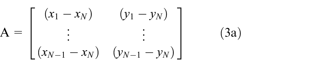
Equation AX = b is solved by least-square method to get the value of x, that is, x = (A^TA)⁻¹A^Tb.

Related work

DV-Hop localization has been considered as one of the primarily used localization algorithms in WSNs. Many researchers have worked on this algorithm to improve its efficiency in terms of complexity and its location accuracy. In the most recent research work,³ the authors have introduced a hybrid three-dimensional node localization algorithm called DV-Hop-AC-PSO. The algorithm combines the advantages of DV-Hop, ant colony, and particle swarm algorithm. In the proposed algorithm, particle swarm has been adopted to optimize the parameters of the ant colony algorithm, and DV-Hop algorithm is used in the iterative process of ant colony algorithm to improve the localization accuracy. The algorithm lacks behind with higher complexity and dependency of other supportive algorithms.

An improved DV-Hop algorithm⁴ has been introduced that uses the weighted average hop distances of anchor nodes with a defined threshold. Weights are calculated to get the average weighted correction factor for the estimation of unknown nodes’ locations. Similarly, a threshold-based improved DV-Hop algorithm has been shown by the researchers in Qian et al.⁵ In this approach, each unknown node initially determines a threshold for selecting the information received. This approach also achieves a minimum error by choosing the optimal number of anchor nodes for location calculation. Other weighted average hop distance based algorithms are also used in Yingjie et al.⁶ and Pan and Liu.⁷

An energy efficient algorithm extended from DV-Hop has been shown in Kumar and Lobiyal.⁸ The anchor nodes communicate only one time with the unknown nodes to inform about the coordinates of the anchor nodes. Calculating of hop size at unknown nodes reduces the communication overhead between anchor nodes and unknown nodes. This results in minimization of the energy consumption. In Kumar and Lobiyal,⁹ the error reduction method has been shown by the authors. The advanced DV-Hop algorithm uses the effective aspects of the parameters. Using the effective distance, estimated locations of unknown nodes are calculated by two-dimensional (2D) hyperbolic location algorithm. The covariance matrix of range estimation error is used as weight matrix for location error improvement. The authors in El Assaf et al.¹⁰ have derived a mechanism to reduce error further. The authors have computed mean hope size at each unaware node which limits the broadcasting of control messages by the anchor nodes. Another improvement on DV-Hop algorithm has been suggested in Chen and Zhang.¹¹ The improvement in locating performance has been done by modifying and weighting the average hop distance between anchor nodes. The particle swarm optimization is used to get the accurate location of the unknown nodes. These weighted methods are efficient in reducing location error but are not validated for a mobile sensor network.

An improved DV-Hop has been introduced in Yu and Li.¹² The calculated error is added to the distance between the anchor nodes and the unknown nodes. A similar approach has been shown in another research in Zhang et al.¹³ It includes the maximum and the minimum values of hop counts to calculate the location error and also use the error in the correction method. A novel localization algorithm called VAH-DV-Hop has been introduced in Liu et al.¹⁴ The algorithm uses angle method to reduce the negative factors which are caused by routing void and finally, trilateration method is used for the location estimation.

Some researchers have suggested the localization estimation responsibility of anchor nodes in neighbors’ proximity. The same has been researched in Li¹⁵ with different average hop values. This approach is static and does not confirm the dynamic scenario in the network. The research work in Dai et al.¹⁶ shows an improvement in DV-Hop with three modifications. First, the secondary reference node is located by three anchor nodes using trilateration or centroid method. Second, modification depends on the node of the last hop, and finally, it uses the Max–Min method.

Various research have been done to check the effect of localization in presence of mobile anchor nodes. The research work in Guerrero et al.¹⁷ has shown azimuthally defined area localization (ADAL). This algorithm utilizes the anchor nodes with mobility. The concept of azimuth and rotary directional antenna has been used for the purpose. The unknown nodes use the centroid mechanism to estimate their location. Though the approach supports mobility but needs specific hardware as a rotary directional antennas. Localization with a mobile anchor node based on trilateration (LMAT) is proposed in Han et al.¹⁸ The algorithm uses mobile nodes that move along the trilateration trajectory.

A recent work in Han et al.¹⁹ has introduced a mobile anchor based localization algorithm called as mobile anchor assisted localization algorithm based on regular hexagon (MAALRH). This algorithm is based on regular hexagonal in 2D WSNs. This algorithm does not perform effectively when nodes are randomly deployed. In the paper,²⁰ the authors describe a localization algorithm called mobile anchor centroid localization (MACL) that uses a single mobile anchor. The localization method is based on radio frequency and therefore, extra hardware cost is not required. The single mobile anchor node does not support complete mobile environment and will be more resource exhaustive if the number of unknown nodes increases. In the work,²¹ Minimum Connected Dominating Set (MCDS) using dominating set has been introduced. The algorithm consists of three phases. The first phase deals with the searching for a dominating set, the second phase identifies the connectors, and the final phase prunes the generated connected dominating set to get the MCDS. Deactivation of nodes due to power constraint is also taken into consideration for this algorithm with repairing process.

All these improvements in DV-Hop work efficiently to localize an unknown node with better precision, but the drawback occurs when both anchor nodes and unknown nodes are mobile. This issue has been addressed in the previous work,^22,23 but it requires rigorous research with the random deployment of the nodes. Therefore, we have developed an algorithm to address these problems of location estimation in the presence of mobile anchors and mobile unknown nodes.

Proposed algorithm

We know that in WSNs, anchor nodes are more privileged in the term of resources and communication as compared to unknown nodes. Thus, utilization of the anchor nodes in an efficient way is the prime goal of our research. In the proposed algorithm, we have considered the unknown nodes in the one-hop neighborhood of each anchor node. Among all the anchor nodes in the set, we have selected only those anchor nodes which are having the maximum degree of connection with one-hop distanced unknown nodes. Such anchor nodes have created the dominating set of anchors. This dominating set acts as the backbone of the network to localize the unknown nodes. Finally, pruning is also used to minimize the size of the backbone consisting of dominating anchor nodes and to avoid redundancy. For example, consider Figure 1.

Figure 1.

Topology and aerial distances among anchor nodes and unknown nodes.

The black color nodes numbered from 1 to 5 are the anchor nodes. All the gray color nodes are the unknown nodes in the network. The maximum degree of connectivity will be calculated for each of the anchor nodes depending upon two considerations: range and one-hop neighbors. If two anchor nodes are having the same degree of connection, one anchor node among them will be randomly chosen for the dominating set at a particular iteration. Considering our algorithm for the above example, let us suppose the anchor node numbered 2 has the maximum degree of connectivity with the unknown nodes as it has six neighbors in its range. Therefore, in the first iteration, anchor node numbered 2 is in the dominating set. Similarly, anchor nodes numbered 1 and 3 also become members of that set. These anchor nodes (1, 2, and 3) are covering all the unknown nodes in their vicinity. Therefore, there is no need of adding anchor node 4 and anchor node 5 in the dominating set. This dominating set is connected and it contains the minimum number of nodes, three (minimum requirement for trilateration) out of five anchor nodes to cover up all the unknown nodes and therefore, it is considered as MCDS.

Backbone generation with anchor nodes

A set of anchor nodes A and a set of unknown nodes U have been initialized. An empty dominating set D is initialized to $Φ$ which further contains the anchor nodes that are the members of MCDS. The maximum degree of the anchor nodes in set A is calculated. The anchor node having the maximum degree of connectivity becomes a member of the dominating set D. The process continues till either all the anchor nodes are the members of D or each unknown node is a one-hop neighbor of anchor nodes present in D. The number of anchor nodes in the dominating set needs to be greater than or equal to three to perform trilateration. Another condition is imposed on the number of anchor nodes, that is, a minimum number of anchor nodes must be three to perform trilateration. Pruning method is used to reduce the size of dominating set such that all the unknown nodes are covered up by the minimum number of anchor nodes. Once MCDS is constructed, trilateration is applied on anchor nodes to get the location estimation of unknown nodes. The process is summarized in Algorithm 1.

Algorithm 1.

Generating backbone with anchor nodes.

procedure LOCATION ESTIMATION FOR UNKNOWN NODES
1. Initialize:- A ← {a₁,a₂,………,a_N} (Anchor Nodes),
2. U ← {u₁,u₂,………,u_n} (Unknown Nodes)
3. where N ≠ n
4. Dominating Set (D) ←

Φ

(Dominating Set is Empty)
5. while {True} do
6. if (∀ a_i∈ D || ∀ u_i∈ (∃ N(a_i)) && (D(a_i) ≥ 3)) then
7. Break while loop if all anchor nodes are in dominating set or all the unknown nodes are one-hop neighbour of any anchor node and No. of anchor nodes in dominating set is ≥ 3
8. else
9. Compute Max degree[A] // calling Max degree[] for the set A
10. D = D ∪ a_d // Generating dominating set with Anchor Nodes
11. {A_j} = {A_j−1} − {a_d}
12. end if
13. end while // Iterate until condition in 7 is achieved
15. Prune (D)
16. Compute Trilateration on the set D
end procedure

Calculation of maximum degree in anchor set

The calculation of maximum degree in the set of anchor nodes has been proposed in Algorithm 2. The anchor node set A is given as input for this algorithm. For each of the anchor nodes in the set A, its degree is initialized to 0. The connection status with unknown nodes is checked for each of the anchor nodes in the network. If the connection status is true, the degree of the corresponding anchor node is increased by 1. Thus, once all the degrees of all the anchor nodes are received, the maximum degree is calculated and the anchor node with the highest degree is processed.

Algorithm 2.

Calculation of maximum degree from anchor set.

procedure ANCHOR NODE HAVING MAXIMUM DEGREE
1. Initialize:- The Anchor Set in algorithm 1 operation 2
2. for all Anchor Node {A} do
3. Initialize deg[a_i] ← 0; \\ where i is the index variable for anchor nodes
4. for all Unknown Nodes {U} do
5. Compute connection status;
6. if connection status = true then
7. deg[a_i] = deg[a_i] + 1;
8. end if
9. end for
10. end for
11. compute Maximum (deg[A]); \\ calculate maximum degree in the set of anchor nodes
12. Return (a_d); \\ return the anchor node having maximum degree
end procedure

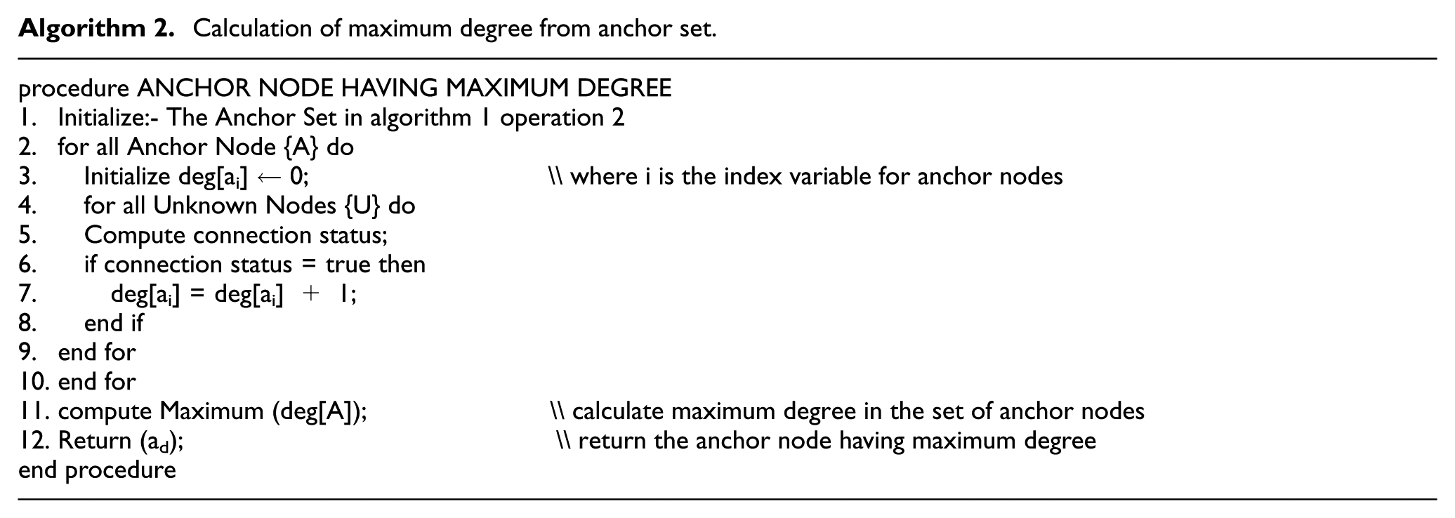
The function of computing connection status between the anchor and unknown node and the calculation of maximum degree are discussed below.

Determining the connection status

The process of checking the connection status between an anchor node and an unknown node is summarized in Algorithm 3. Each anchor node broadcasts a ReQest Neighbour Set (RQNS) packet, which consists the source address (SrcAddr), leash count variable (Leash_C), the sequence number of the request packet (I_SEQ), and acceptance status (Accept_S). The variable Leash_C is used to control hop count to 1 and therefore initialized to 1. Accept_S is initialized to 0. On receiving RQNS, each unknown node, who is in one-hop neighborhood of anchor node, replies with RePly Neighbourhood Set (RPNS): {SrcAddr, Leash_C = 0, I_SEQ, Accept_S = 1, U_Addr}. U_Addr is the address of the unknown node from where the RPNS is coming to the corresponding anchor node. After receiving the RPNS, the anchor node checks the values of Accept_S and Leash_C. If Accept_S = 1 and Leash_C = 0, then the anchor node enlists the corresponding U_Addr as its one-hop neighbor.

Algorithm 3.

Checking connection status between anchor node and unknown node.

procedure CONNECTION STATUS BETWEEN a_i AND u_j
1. Input Anchor Node a_i and Unknown Node u_j
2. Broadcast by Anchor Node a_i
3. Send RQNS : {SrcAddr,Leash_C = 1,I_SEQ,Accept_S = 0}
4. On Receiving node u_j Compute
5. Leash_C = Leash_C − 1;
6. Accept_S = 1
7. Send RPNS : {SrcAddr,Leash_C,I_SEQ,Accept_S,U_Addr}
8. if (Leash_C = 0 && Accept_S = 1) then
9. Return True;
10. Else
11. Return False;
12. end if
end procedure

Function returning index of anchor node having maximum degree

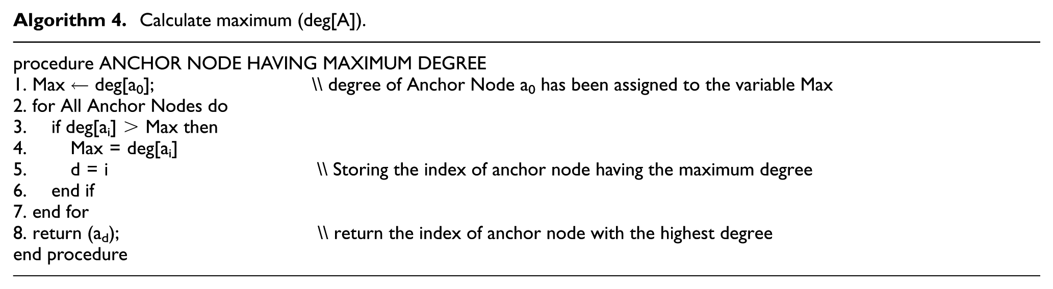
An array consisting of the degrees of all anchor nodes has been taken as input to calculate the maximum degree. The first anchor node’s degree is initialized to be the maximum and then compared with rest of all anchor nodes’ degrees. Finally, the index of the node having a maximum degree is returned to Algorithm 1. The method is shown in Algorithm 4.

Algorithm 4.

Calculate maximum (deg[A]).

procedure ANCHOR NODE HAVING MAXIMUM DEGREE
1. Max ← deg[a₀]; \\ degree of Anchor Node a₀ has been assigned to the variable Max
2. for All Anchor Nodes do
3. if deg[a_i] > Max then
4. Max = deg[a_i]
5. d = i \\ Storing the index of anchor node having the maximum degree
6. end if
7. end for
8. return (a_d); \\ return the index of anchor node with the highest degree
end procedure

Pruning process

It may happen that single unknown node is a neighbor of more than one anchor node. Pruning method is used to avoid redundancy of nodes so that the dominating set D is composed of the minimum number of anchor nodes. The method is shown in Algorithm 5. It returns the MCDS which acts as the backbone to locate the unknown nodes.

Algorithm 5.

Pruning of dominating set D.

procedure MINIMUM DOMINATING SET
1. Input Dominating Set D
2. if (D(a_i) > 3) then \\ No. of anchor nodes in dominating set D is greater than 3
3. min ← min_degree(D)
4. if N[min] N[a₁] ∪ N[a₂] ∪ …… ∪ N[a_N] then
5. D = D − {min};
6. Prune(D); \\ Recursively call Prune after deleting min from dominating set
7. else
8. Prune(D − {min}) \\ Recursively call Prune excluding min but not deleting from dominating set
9. end if
10. return D
11. else
12. return D
13. end if
end procedure

Network model

The sensor network is modeled using a graph G = (V, E) where V represents the nodes (both the anchor and unknown nodes) and E represents the connectivity set. Considering a as anchor node, u as an unknown node and a, u ∈ V, (a, u) ∈ E iff a and u are within one-hop neighborhood transmission range. The dominating set of graph G is $D \subseteq V$ such that D consists of only anchor nodes and each non-anchor node in V is a one-hop neighbor of at least one anchor node in D. A connected dominating set for a given graph G is a dominating set D with the feature that the nodes in D must create a connected subgraph. The MCDS for the graph G can be defined as a dominating set $D \subseteq V$ such that D consists of only the minimum number of anchor nodes and all non-anchor nodes in V are one-hop neighbor of at least one anchor node in D.

The features of the nodes and the overall network take part to create a significant effect on the efficiency of localization. We have considered such features as design parameters of our proposed localization algorithm including connectivity, transmission range, and local stability. Each of these metrics has its own priority depending on the service or application. Parametric weights are therefore needed to be included with those design parameters.

Node degree

Each anchor node computes its degree of connectivity with its neighbor nodes as defined in Algorithm 3. The degree of an anchor node a is the total number of unknown nodes within its one-hop distance and is computed as

De g_{a} = \sum_{a \in V, a \neq u} {ho p_{a, u} = 1}

(4)

where Deg_a is the total degree of an anchor node, $ho p_{a, u}$ is the one-hop distance between anchor node a and unknown node u.

Transmission range

The transmission range T_r of an anchor node is dependable on the application scenario.²⁴ As network scenario is considered to be dynamic, transmission range varies within the interval of minimum range T_rmin and maximum range T_rmax. The transmission range T_r is therefore given by

T_{r} = T_{rmin} + Random (0, 1) \times (T_{rmax} - T_{rmin})

(5)

where Random (0, 1) generates a randomized number between 0 and 1.

In our experimentation, we have used three variable scenarios for anchor nodes with minimum and maximum transmission range as (20, 40), (30, 50), and (40, 60), respectively. The transmission range of the unknown nodes is fixed at 35.

Mobility

To compute the mobility, each anchor node in the dominating set requires to calculate the distance from its neighboring unknown nodes. For this purpose, Friis free space propagation model²⁵ is used. The received power P_r is computed as

P_{r} = P_{t} \times G_{t} \times G_{r} \times \frac{λ^{2}}{{(4 \times π \times Dist)}^{2}}

(6)

where P_r is the power received by the receiving antenna of the anchor node, P_t is the power input to the transmitting antenna, G_t and G_r are the transmitting gain and receiving gain, respectively, $λ$ is the wavelength and $Dist$ is the distance with the condition P_r is inversely proportional to the square of the distance. An approximate distance at time t between an anchor node a ∈ dominating set D and an unknown node u is calculated as

{Dist}_{t}^{a, u} = \frac{k}{\sqrt{P_{r}}}

(7)

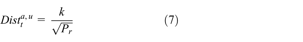
where k is constant and ${Dist}_{t}^{a, u}$ is the distance between a and u at time t.

Relative mobility in the network indicates whether any two nodes are coming closer to or moving away from each other. The relative mobility of an unknown node u with respect to anchor node a at a given time t is given by

{RM}_{t}^{a, u} = {Dist}_{t}^{a, u} - {Dist}_{t - 1}^{a, u}

(8)

${RM}_{t}^{a, u}$ is positive if node u is moving away from a and negative if u is coming closer to a. The distance from a to u is measured at certain time interval for T times and we get the values ${RM}_{1}^{a, u}$ , ${RM}_{2}^{a, u}$ ,…, ${RM}_{T}^{a, u}$ . The standard deviation of relative mobility (SD_RM) defines the variation of the distances over a period of time T as

S D_{RM} = \sqrt{\frac{\sum_{i = 1}^{T} {(R M_{i} - \bar{RM})}^{2}}{T}}

(9)

where

\bar{RM} = \frac{1}{T} ({RM}_{1}^{a, u} + {RM}_{2}^{a, u} + \dots + {RM}_{T}^{a, u})

(10)

Implementation and results

In the simulation process, we have considered the number of nodes as 25, 50, 75, and 100, respectively. We have compared our proposed approach and he original DV-Hop algorithm in Figure 2. We have used variable transmission range. The results show the number of anchor nodes required in the backbone for localization process of the unknown nodes. The DV-Hop algorithm and proposed algorithm have been compared on this aspect. Through results, we can observe that proposed algorithm generates a better result, that is, less number of anchor nodes are able to localize all the unknown nodes. The simulation data of proposed algorithm have been statistically analyzed.

Figure 2.

Localization of unknown nodes with different transmission ranges.

Simulation-based results

The localization error is inexorable in evaluations. We have considered two metrics to calculate the localization error. The metrics can be described as follows.

Average localization error

It is defined as the ratio of the difference between estimated location and the actual location of all the nodes

Average Localization Error = \frac{1}{n} \sum_{i = 1}^{n} \sqrt{{(x_{i} - x)}^{2} + {(y_{i} - y)}^{2}}

(11)

Root mean square error

It is defined as the mean square root of squared differences of estimated location and the actual location

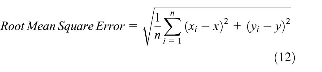
Root Mean Square Error = \sqrt{\frac{1}{n} \sum_{i = 1}^{n} {(x_{i} - x)}^{2} + {(y_{i} - y)}^{2}}

(12)

where (x, y) are actual locations, (x_i, y_i) are estimated locations, and n denotes the number of unknown nodes. The average localization error for different transmission range with variable anchor and unknown nodes has been shown in Table 1. The table also shows the comparison of the average localization error percentage with the algorithm described in Di Franco et al.²²

Table 1.

Average error percentage for different transmission ranges with variable number of unknown nodes.

Transmission range	No. of anchor nodes	Average localization error (%) for all the scenarios of 20, 40, 60, 80, and 100 unknown nodes for DV-Hop algorithm shown in Niculescu and Nath²	Average localization error (%) for all the scenarios of 20, 40, 60, 80, and 100 unknown nodes for algorithm shown in Di Franco et al.²²	Average localization error (%) for all the scenarios of 20, 40, 60, 80, and 100 unknown nodes for the proposed algorithm
20, 40	5	28.766	15.345	10.113
	10	27.977	15.119	9.762
	15	27.031	14.876	8.001
	20	26.433	13.001	7.997
30, 50	5	27.666	14.997	8.321
	10	26.500	14.111	8.007
	15	25.333	12.003	7.147
	20	24.001	11.911	6.009
40, 60	5	26.336	12.001	8.121
	10	25.533	11.099	6.735
	15	24.877	11.001	5.989
	20	24.933	10.998	5.333

Statistical analysis of error improvement

The objective of the statistical analysis is to check whether our introduced algorithm is providing an error improvement over the DV-Hop algorithm or not. To examine this, we have set our hypothesis as per the following:

H₀: There is no improvement of localization error in our algorithm as compared to the DV-Hop algorithm.

H₁: There is a significant improvement of localization error in our algorithm as compared to the DV-Hop algorithm.

To test the above hypothesis, the NS2 simulated data are processed for paired T-test with 0.05 of significance level. We have executed the paired T-test on the average localization error and root mean square error of DV-Hop algorithm and the proposed algorithm. The application of paired T-test has provided the following results shown in Table 2.

Table 2.

Paired T-test results for proposed algorithm and DV-Hop algorithm.

Number of unknown nodes	p-Values (sig. two-tailed) of paired T-test for average mean error	p-Values (sig. two-tailed) of paired T-test for root mean square error
25	0.001	0.000
50	0.000	0.001
75	0.000	0.000
100	0.000	0.000

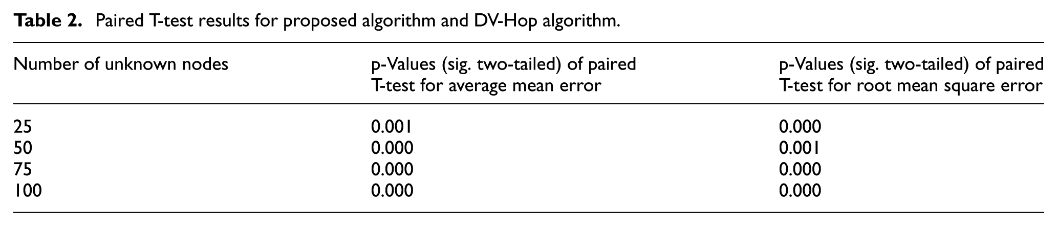
In the above results of paired T-test, it is observed that all the p-values (sig. two-tailed) are <0.05 of significance level. Therefore, the null hypothesis H₀ has been rejected and the alternate hypothesis H₁ has been accepted. It means that there is a significant improvement using the proposed algorithm over DV-Hop algorithm with respect to average localization error and root mean square error for location estimation. Similarly, the above test is also applied to the algorithm shown in Di Franco et al.²² and in comparison with our algorithm. We have found the following result shown in Table 3:

H₀: There is no improvement of localization error in our algorithm as compared to the algorithm shown in Di Franco et al.²²

H₁: There is a significant improvement of localization error in our algorithm as compared to the algorithm in Di Franco et al.²²

Table 3.

Paired T-test results for proposed algorithm and algorithm shown in Di Franco et al.²²

Number of unknown nodes	p-Values (sig. two-tailed) of paired T-test for average mean error	p-Values (Sig. two-tailed) of paired T-test for root mean square error
25	0.000	0.000
50	0.000	0.000
75	0.000	0.000
100	0.000	0.000

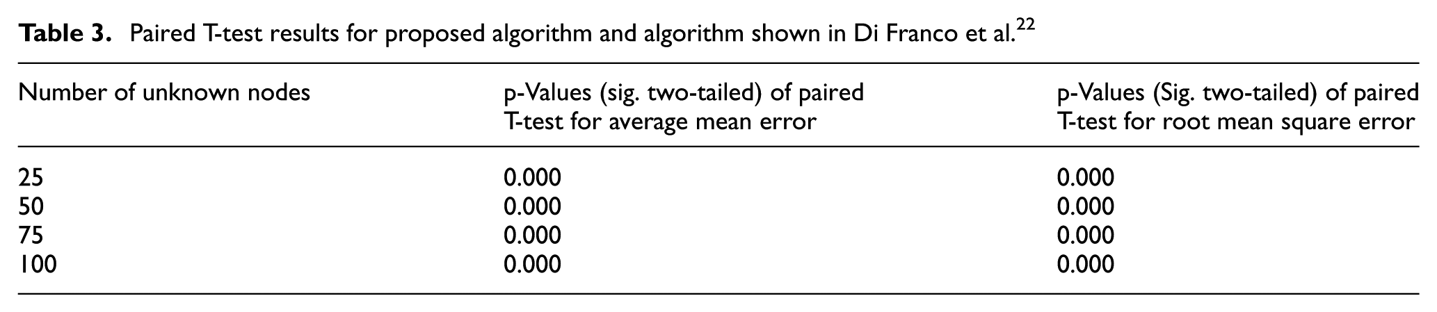
The above result describes that as all the p-values are 0 which is <0.05, it signifies that H₀ is rejected and H₁ has been accepted. It means that there is a significant improvement of error using the proposed algorithm as compared to the algorithm shown in Di Franco et al.²²

Statistical analysis of time consumption

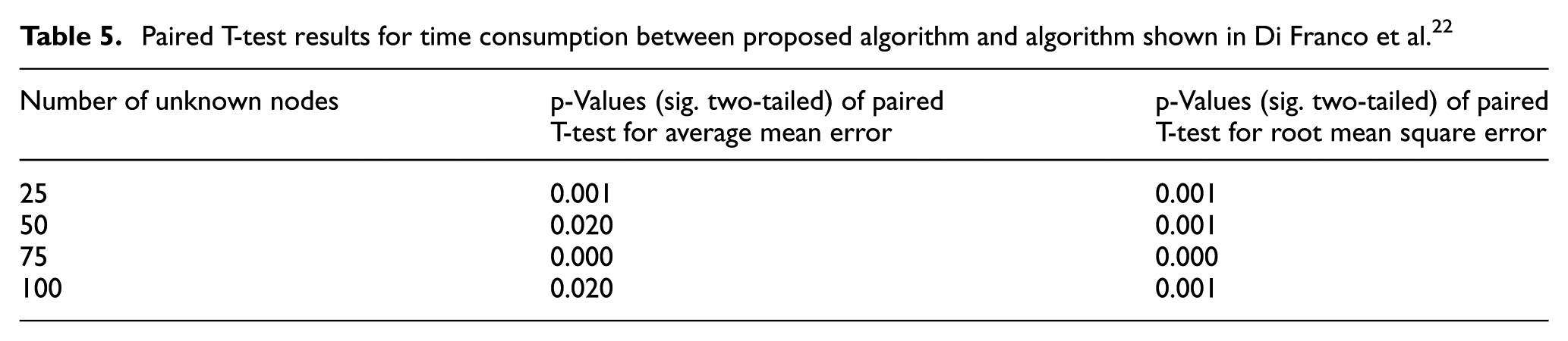
Considering the scenarios of 25, 50, and 75 nodes, the standard error of the differences between the time consumption of DV-Hop algorithm and the time consumption of proposed algorithm is 0 and therefore, a p-value cannot be computed. It means that the time for localization is neither degraded nor upgraded using the proposed algorithm. But it is noticed in the results of 100 nodes given in Table 4 that the p-value is 0 which is <.05 of significance level. It means that the algorithm is also providing an improvement in time consumption of localization. Similarly, the comparison between the proposed work and the algorithm²² has also been done in Table 5. All the p-values are significance level of <.05; therefore, it clearly shows that the proposed work has provided a significant improvement in time consumption over the algorithm in comparison.

Table 4.

Paired T-test results for time consumption between proposed algorithm and DV-Hop.

Number of unknown nodes	p-Values (sig. two-tailed) of paired T-test for time variable
25	Cannot be determined as standard error of the difference is 0
50	Cannot be determined as standard error of the difference is 0
75	Cannot be determined as standard error of the difference is 0
100	0.000

Table 5.

Paired T-test results for time consumption between proposed algorithm and algorithm shown in Di Franco et al.²²

Number of unknown nodes	p-Values (sig. two-tailed) of paired T-test for average mean error	p-Values (sig. two-tailed) of paired T-test for root mean square error
25	0.001	0.001
50	0.020	0.001
75	0.000	0.000
100	0.020	0.001

Conclusion

In this article, an algorithm for localization in a WSN by effectively utilizing anchor nodes is proposed. The algorithm uses the concept of MCDS with anchor nodes, which can cover all the unknown nodes for location estimation. The mobility factor for both the anchor nodes and unknown nodes is considered for the algorithm which can be used for wide range of applications. Simulation results show the efficiency of the proposed algorithm that achieves approximately 92.37% accuracy level of estimated location of unknown nodes along with the random mobility. In future, we shall try to optimize the backbone for considering the energy consumption.

Footnotes

Handling Editor: Salvatore Serrano

Declaration of conflicting interests

The author(s) declared no potential conflicts of interest with respect to the research, authorship, and/or publication of this article.

Funding

The author(s) received no financial support for the research, authorship, and/or publication of this article.

ORCID iD

Mritunjay Kumar Rai

Gulshan Kumar

References

Han

Duong

et al . Localization algorithms of Wireless Sensor Networks: a survey. Telecommun Syst 2013; 52(4): 2419–2436.

Niculescu

Nath

. DV based positioning in ad hoc networks. Telecommun Syst 2003; 22(1–4): 267–280.

Xiao

Zheng

. Research of three-dimensional localization algorithm based on DV-Hop AC-PSO. In: Proceedings of the 26th Chinese control and decision conference (CCDC 2014), Changsha, China, 31 May–2 June 2014. New York: IEEE.

. An improvement of DV-Hop localization algorithm for wireless sensor networks. Telecommun Syst 2013; 53(1): 13–18.

Qian

Shen

Chen

. An improved node localization algorithm based on DV-Hop for wireless sensor networks. Comput Sci Inf Syst 2011; 8(4): 953–972.

Yingjie

Kai

Shenfang

et al . Research of WSN node localization algorithm based on weighted DV-HOP. In: Proceedings of the 24th Chinese control and decision conference (CCDC), Taiyuan, China, 23–25 May 2012, pp.3826–3829. New York: IEEE.

Pan

Liu

. Wireless sensor networks based on the DV-Hop localization algorithm. In: Proceedings of the 4th international conference on computational and information sciences, Chongqing, China, 17–19 August 2012, pp.1073–1075. New York: IEEE.

Kumar

Lobiyal

. Power efficient range-free localization algorithm for wireless sensor networks. Wirel Netw 2013; 20(4): 681–694.

Kumar

Lobiyal

. An advanced DV-Hop localization algorithm for wireless sensor networks. Wireless Pers Commun 2012; 71(2): 1365–1385.

10.

El Assaf

Zaidi

Affes

et al . Hop-count based localization algorithm for wireless sensor networks. In: Proceedings of the 13th Mediterranean microwave symposium (MMS), Saida, Lebanon, 2–5 September 2013, vol. 1, no. 6, pp.2–5. New York: IEEE.

11.

Chen

Zhang

. Improved DV-Hop node localization algorithm in wireless sensor networks. Int J Distrib Sens N. Epub ahead of print 1 January 2012. DOI: 10.1155/2012/213980.

12.

. An improved DV-Hop localization method in wireless sensor networks. In: Proceedings of the 2012 IEEE international conference on computer science and automation engineering (CSAE), Zhangjiajie, China, 25–27 May 2012, vol. 3, pp.199–202. New York: IEEE.

13.

Zhang

Liu

Wang

et al . DV-Hop localization algorithms based on centroid in wireless sensor networks. In: Proceedings of the 2nd international conference on consumer electronics, communications and networks (CECNet), Yichang, China, 21–23 April 2012, pp.3216–3219. New York: IEEE.

14.

Liu

Wang

Shang

. An improving localization algorithm for wireless sensor networks based on DV-Hop. In: Proceedings of the international conference on measurement, information and control (MIC), Harbin, China, 18–20 May 2012, pp.511–515. New York: IEEE.

15.

. Improved DV-HOP location algorithm based on local estimating and dynamic correction in location for wireless sensor networks. Int J Digit Content Technol Appl 2011; 5(8): 196–202.

16.

Dai

Wang

Zhang

. Improvement of DV-Hop localization algorithms for wireless sensor networks. In: Proceedings of the 6th international conference on wireless communications networking and mobile computing (WiCOM), Chengdu, China, 23–25 September 2010, pp.23–25. New York: IEEE.

17.

Guerrero

Xiong

Gao

et al . ADAL: a distributed range-free localization algorithm based on a mobile beacon for wireless sensor networks. In: Proceedings of the international conference on ultra modern telecommunications & workshops, St. Petersburg, Russia, 12–14 October 2009, pp.1–7. New York: IEEE.

18.

Han

Jiang

et al . Path planning using a mobile anchor node based on trilateration in wireless sensor networks. Wirel Commun Mob Com 2013; 13(14): 1324–1336.

19.

Han

Zhang

Lloret

et al . A mobile anchor assisted localization algorithm based on regular hexagon in wireless sensor networks. Sci World J 2014; 2014: 219371.

20.

Song

et al . Localization in wireless sensor networks using a mobile anchor node. In: Proceedings of the IEEE/ASME international conference on advanced intelligent mechatronics (AIM 2008), Xian, China, 2–5 July 2008. New York: IEEE.

21.

Rai

Verma

Tapaswi

. A power aware minimum connected dominating set for wireless sensor networks. J Network 2009; 4(6): 511–519.

22.

Di Franco

Franchino

Marinoni

. Data fusion for relative localization of wireless mobile nodes. In: Proceedings of the 9th IEEE international symposium on industrial embedded systems (SIES), Pisa, 18–20 June 2014. New York: IEEE.

23.

Chenji

Stoleru

. Mobile sensor network localization in harsh environments. In: Proceedings of the international conference on distributed computing in sensor systems (DCOSS), Santa Barbara, CA, 21–23 June 2010. Berlin; Heidelberg: Springer.

24.

Tang

Yang

et al . An energy efficient MCDS construction algorithm for wireless sensor networks. EURASIP J Wirel Comm 2012; 2012: 83.

25.

http://www.antenna-theory.com/basics/friis.php

An improved DV-Hop localization with minimum connected dominating set for mobile nodes in wireless sensor networks

Abstract

Keywords

Introduction

DV-Hop localization

Related work

Proposed algorithm

Backbone generation with anchor nodes

Calculation of maximum degree in anchor set

Determining the connection status

Function returning index of anchor node having maximum degree

Pruning process

Network model

Node degree

Transmission range

Mobility

Implementation and results

Simulation-based results

Average localization error

Root mean square error

Statistical analysis of error improvement

Statistical analysis of time consumption

Conclusion

Footnotes

Declaration of conflicting interests

Funding

ORCID iD

References