
Abstract
The high attenuation of radio signals in water leaves acoustic waves the most viable communication media for underwater sensor networks. Nevertheless, acoustic communication suffers from significantly high latency because of its low propagation speed compared to radio communication. In this article, we consider the problem of constructing connected dominating sets as virtual backbones under acoustic communication. We abstract a wireless sensor network as a graph with weighted edges, where the weight of an edge represents the latency between the wireless nodes it links. Three approximation algorithms are proposed to optimize the latency of a connected dominating set. The first algorithm provides a two-approximation to the diameter of a connected dominating set, where the diameter is defined as the length of the longest shortest path in a graph. The second algorithm guarantees a six-approximation to the minimum latency between any pair of nodes and meanwhile has constant approximations to the connected dominating set size in unit disk graphs and unit ball graphs. The third algorithm constructs a connected dominating set with 12-approximation to the diameter and 10.197-approximation to the size in unit disk graphs. Extensive simulations are carried out to validate the performance of the proposed algorithms.
Introduction
The growing need for ocean observation systems has stimulated considerable interest on the study of underwater sensor networks (USNs). A USN consists of underwater sensor nodes, which cooperatively work together to offer a wide spectrum of applications,1–4 such as pollution monitoring, oceanographic data collection, and coastline protection. To make these applications viable, there is a need to enable underwater communications among underwater devices.
Wireless underwater acoustic networking is the enabling technology for these USN-based applications. In fact, electromagnetic waves propagate for long distances through sea water only at extra low frequencies (30–300 Hz), 5 which requires large antennae and high transmission power. By comparison, acoustic waves do not have such high attenuation in water, so that a USN differs from terrestrial sensor networks that it relies on acoustic signals for communication. However, acoustic communication suffers from critically high latency and long end-to-end delay because of its low propagation speeds (1.5 × 10³ m/s) compared to radio communication (3 × 10⁸ m/s).
In wireless sensor networks, a lot of effort has been made on constructing a virtual backbone (VB) 5 for efficient routing and network topology control. Due to the limited transmission range of sensor nodes, node-to-node communication in sensor networks usually follows a multi-hop pattern with the help of some intermediate relay nodes. That is to say, routing in sensor networks is about finding appropriate relay nodes for passing messages. Once a VB is used in a wireless sensor network, the routing tasks are restricted to the backbone nodes. A small size VB suffers less from interference and leads to more efficient energy consumption and simpler routing maintenance when network topology changes.
Unfortunately, the use of VBs also increases the latency of the network. The high latency of acoustic communication makes this problem more severe in USNs than in terrestrial sensor networks. In this article, we consider the problem of constructing latency-optimal VBs using acoustic communication. Currently, connected dominating set (CDS)-based approaches have become one of the most competitive VB construction methods in sensor networks. In a wireless sensor network abstracted as a graph
In this article, a wireless network is abstracted as an undirected graph with weighted edges, where the weight of an edge represents the latency between the sensor nodes it links. As some previous works,6–9 we model a homogeneous wireless network as a unit disk graph (UDG) or a unit ball graph (UBG). A USN can be represented as an edge-weighted UBG because it naturally distributes in a three-dimensional (3D) underwater area. In addition, some monitoring missions require all underwater nodes deployed in the same depth, 10 in which case a wireless network can be represented as an edge-weighted UDG.
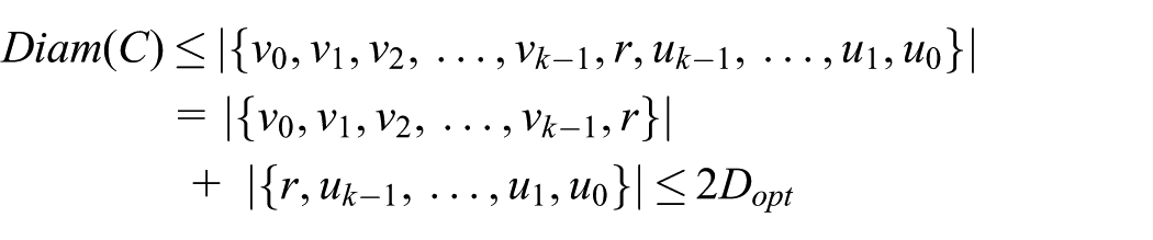
Figure 1 presents an example of an edge-weighted UDG. In Figure 1, if

An edge-weighted unit disk graph.
Three algorithms are proposed in this article:
The first algorithm is devised for general graphs and achieves a two-approximation to the diameter of a CDS. The diameter of a graph is defined as the length of the longest shortest path in it. That is, if C is a CDS of
Considering that the first algorithm does not guarantee desirable approximation ratio to CDS size, we devise the second algorithm and the third algorithm which have constant approximation ratios to CDS size in UDGs and UBGs. For any pair of nodes with minimum latency
Considering that approximation ratio to CDS size of the second algorithm is big, we devise the third algorithm which provides a 12-approximation to CDS diameter, and meanwhile a 10.197-approximation to CDS size in UDGs.
The proposed algorithms are summarized in Table 1, which shows that theoretically (1) the first algorithm is more suitable for networks demanding that the latency between a pair of nodes would not be too bad in the worst case, (2) the second algorithm is more suitable to be used when the latency between any pair of nodes is needed to be concerned, and (3) the third algorithm is promising when backbone size and latency are both important to operate the network.
Approximation ratio of the proposed algorithms.

Besides USNs, the proposed algorithms can also apply to other kinds of networks with high point-to-point delays, such as delay tolerant networks and large-area sensor networks. However, USNs are the most typical and reasonable networks to apply the proposed algorithms because of the high latency of acoustic communication. Therefore, we only discuss about the CDS problem in USNs in this article and the approaches can be simply extended to other target scenes.
The rest of this article is organized as follows.
A brief review for CDS construction algorithms is presented in section “Related work.” In “Problem statements,” we introduce the assumptions and formalize the problem. Details of the proposed algorithms are shown in sections “The first algorithm,”“The second algorithm,” and “The third algorithm.” Extensive simulations are conducted and the results are presented in section “Simulation.” Finally, we conclude this article in section “Conclusion.”
Related work
We briefly review existing CDS construction algorithms in this section by three categories: algorithms optimizing the size, algorithms optimizing the routing cost, and algorithms optimizing other parameters. Readers can refer to Du and Wan 11 for more comprehensive introductions about CDS construction algorithms.
CDS algorithms optimizing the size
Most of existing CDS algorithms focus on constructing a minimum size CDS. Guha and Khuller
12
proposed two approximation algorithms in general graphs. Their first algorithm grows a spanning tree as the dominating tree by the node with the maximum degree. Their second algorithm contains two phases, with the first phase to construct a DS and connects it in the second phase. These algorithms achieve performance ratio
In addition to these MIS-based algorithms, some marking-based algorithms are proposed in Dai and colleagues.21,22 These algorithms first mark a CDS and then prune redundant nodes to obtain a small size. Compared to MIS-based algorithms which usually have polynomial time complexities, the marking-based algorithms do not guarantee constant approximation ratios, but are localized with
For wireless networks composed of nodes equipped with directional antennas, the network can be modeled as a graph with directional links. The CDS problem on directional network models has been studied in Wu and colleagues.23,24
CDS algorithms optimizing the routing cost
Some existing works optimize the routing path lengths of a CDS in wireless sensor networks. Ding et al. 25 proposed an algorithm to construct a minimum routing cost CDS (MOC-CDS). Their algorithm guarantees that each routing path between any pair of nodes is also the shortest path in the network. Their key idea is based on the observation that a MOC-CDS is equivalent to a 2hop-CDS, which ensures that for any two nodes with distance equal to 2, there exists at least one shortest path between them. Ding et al. 26 extended the MOC-CDS problem to an α-MOC-CDS, which guarantees α-approximations to the routing path length between any pair of nodes. Liu et al. 27 considered to optimize the CDS routing cost in heterogeneous wireless networks. Du et al. 28 proposed an MIS-based approach which guarantees constant approximation ratio to both CDS size and routing path length between any pair of nodes. Kim et al. 29 proposed two algorithms to optimize the diameter of a CDS. Their algorithms guarantee constant approximation ratio to both the size and diameter of a CDS.
Algorithms optimizing other characteristics of a CDS
There are also many works considered to optimize other characteristics of a CDS, such as load balancing, network lifetime, and fault tolerance.
For algorithms optimizing other parameters of a CDS, He et al. 30 suggested to construct a load-balanced CDS to balance the communication overhead of backbone nodes. Alzoubi et al. 31 proposed a distribute algorithm to optimize the message complexity while ensuring constant approximation in terms of CDS size.
Some applications assume that sensor nodes have different weights, where the weight of a node usually represents its remaining energy. Hence, an important line of works studies the problem of constructing a minimum weight CDS (MWCDS). The MWCDS problem plays an important role for the study of maximum lifetime problem in wireless sensor networks. In fact, Garg and Koenemann 32 proved that if the minimum weight sensor cover problem has a ρ-approximation, then the maximum lifetime problem will have a (ρ + ε)-approximation. For the construction of a MWCDS, interested readers can refer to the literature.9,33,34
Dai and Wu 35 initially discussed about constructing a k-connected m-dominating set ((k,m)-CDS) as a fault-tolerant VB. A (k,m)-CDS can survive after any k − 1 backbone nodes fail. A non-backbone node can connect to the VB even after its m − 1 adjacent backbone nodes fail. Dai and Wu 35 proposed three algorithms to construct a (k,k)-CDS, but no performance ratio was analyzed. Approximation algorithms with constant performance ratio to construct a (k,m)-CDS in UDGs have been studied previously.36–39 Zhang et al. 40 proposed a performance-guaranteed algorithm for the minimum (3,m)-CDS problem in a general graph.
Some works consider to construct a CDS under other communication models. Yu et al. 7 discussed about CDS construction under the beeping model, which is a novel communication model compared to the traditional message passing model. Wu et al. 41 studied the CDS problem under the cooperative communication model. Dai et al.42,43 studied the backbone problem in cognitive radio networks.
Discussion
The differences between this article and existing works are twofold. First, for weighted graphs, existing works suppose that sensor nodes are weighted to represent the remaining energy. Instead, this work uses the weight of a link between nodes to represent latency caused by acoustic communication and motivates to optimize the routing cost instead of network lifetime. Second, existing routing cost optimization CDS algorithms measure the length of a routing path by the hop-distance among sensor nodes. Thus, the theoretical analyses for these algorithms are inappropriate for edge-weighted graphs. In addition, more proper implementations should be proposed for acoustic communication-based wireless networks.
Problem statements
We use an edge-weighted UDG
With acoustic communication, the latency between a pair of adjacent nodes can be obtained through two schemes:
If all sensor nodes are well synchronized, then the end-to-end delay between two adjacent nodes can be tested through passing messages with time stamps.
If the sensor nodes are not well synchronized, the communication latency between two neighboring nodes can also be estimated by their locations with some simple assumptions. For underwater sensor node localization, interested readers can refer to Liu et al.
10
For a pair of adjacent sensor nodes
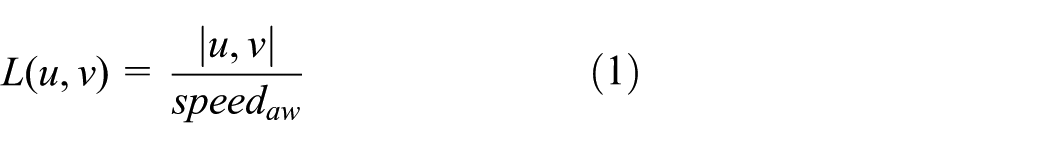
Let
We assume that 1 unit distance causes 1 unit latency. Thus, hereafter, in this article, the weight of
We use

Hence, the minimum latency between two arbitrary nodes
Suppose
The first algorithm
Algorithm description
The basic idea of the first algorithm is to build a dominating tree, where every node in the network retransmits the flooding message when it is the first time to receive it. It can be proved that the dominating tree is also a shortest path tree, which means it provides a shortest routing path from root to each node in the network. Since a shortest path tree provides routing of at most two-approximation to the diameter of the graph, the first algorithm also guarantees a two-approximation to optimal CDS diameter. Note that traditional shortest path algorithms, such as Dijkstras algorithm and Floyd–Warshall algorithm, require the entire topology information of a graph and have running time at least
In Step 1 of the first algorithm, the node with the smallest ID initiates the flooding process. An

Theorem 1
Black nodes outputted from Algorithm 1 form a CDS of
Proof
Any node in
Performance analysis
In Theorem 2, we prove that the dominating tree is a shortest path tree, which guarantees a two-approximation to CDS diameter (equation (4)).
Theorem 2
If

where
Proof
For any node
Now, we prove by contradiction that the path
Therefore, for any node
Theorem 3
The time complexity and message complexity of the first algorithm are
Proof
In the first algorithm, a node sends the INVITE message when it is the first time to receive the message. In Theorem 2, we have proved that the INVITE message reaches a node through the shortest path from the leader node. Therefore, the algorithm ends in
Observe that the first algorithm does not guarantee any approximation ratio in terms of CDS size. In the rest of this article, we introduce the other two approximation algorithms which not only optimize routing path length of a CDS but also ensure constant approximation ratio in terms of CDS size.
The second algorithm
Algorithm description
The second algorithm follows an MIS-based two-phased approach. In the first phase, an MIS is constructed as a DS. In the second phase, each pair of MIS nodes within three hops is connected. The idea of the second algorithm is inspired by Alzoubi et al. 31 and Du et al. 28 Alzoubi et al. 31 used such a scheme to optimize the message complexity of a CDS algorithm. Du et al. 28 proved that the routing cost of the scheme is guaranteed. However, the routing cost in Du et al. 28 is defined as the hop-distance between a pair of nodes, which is different from this article. In this section, we show that using the shortest three-path (will be defined later) to connect MIS nodes, a constant approximation ratio to CDS size and routing cost can both be guaranteed in edge-weighted graphs.
Definition 1 (independent set)
For a graph
Definition 2 (MIS)
An IS of
An MIS is also a DS. The MIS is used in the second algorithm because some previous works have studied and presented upper bounds of MISs to the size of a minimum CDS6,8,13–15,17,18 in UDGs and UBGs. According to these works, we can provide theoretical analysis for the size of the constructed CDS.
In the second algorithm, a node in the MIS is colored in black. For an MIS
The shortest path between
We connect each pair of neighboring black nodes by the shortest three-path between them, where the shortest three-path is defined as the shortest path between two nodes with at most three edges. We stress that a shortest three-path may not be the shortest path between two neighboring black nodes, because a four-hop path may be the shortest path between two three-hop black nodes. As shown in Figure 2, the shortest path between nodes
The second algorithm can be summarized as follows:
Phase 1: Construct an MIS and color its nodes in black.
Phase 2: Connect each pair of neighboring black nodes by the shortest three-path between them.
Algorithm 2 describes the second algorithm in a distributed pattern.

In Steps 1–6 of Algorithm 2, an MIS is constructed by the algorithm introduced in Alzoubi et al.
31
The main idea of this MIS construction algorithm is if all neighbors of a node with larger identifiers have decided not to join the MIS, then the node decides to join the MIS. In Steps 5 and 6, a node sends the
Theorem 4
The black and blue nodes outputted from the second algorithm form a CDS of
Proof
First, the black and blue nodes form a DS of
Performance analysis
Next, we show some theoretical analyses to evaluate the performance of the second algorithm. In order to analyze the latency of a CDS constructed by the second algorithm, we first introduce a fact as follows.
Fact 1
Given three adjacent nodes

Hereafter, in this article, for a set of black MIS nodes

where
In fact, the second algorithm generates a CDS with all the black paths of
Theorem 5
For any two nodes
If

If k is an odd number, then

Proof
We use
When

For any

such that

When
For any

such that

This completes the proof.

On the proof of Theorem 5.
Corollary 1
For any two nodes in
Proof
The second algorithm constructs a CDS with all the black paths in it. According to Theorem 5, the corollary holds.
To analyze the approximation ratio of the second algorithm in terms of CDS size, we introduce some lemmas first.
Lemma 1
In a UDG, a node has at most 41 independent neighbors within three-hops.
Proof
As shown in Figure 4, the problem of the lemma can be solved referencing a classical mathematical problem, the circle packing in a circle problem. Observe that the result of the lemma equals to the following problem: how many unit circles can be packed in a bigger circle with radius 7? Alzoubi et al. 31 proved an upper bound 47 of this problem. Du et al. 28 improved this result to 43. We find that this result can be further improved to 41 according to Gáspár and Tarnai. 44 We refer to Gáspár and Tarnai 44 for readers interested in detail.

The problem of Lemma 1 is equivalent to another problem that packing as many circles with 0.5 radius as possible in a bigger circle with radius 3.5. And it is further equivalent to the problem that packing as many unit circles as possible in a bigger circle with radius 7.
Lemma 2
In a UBG, a node has at most 267 independent neighbors within three-hops.
Proof
As the proof of Lemma 1, the result of this lemma can be proved by the sphere packing in a sphere problem. The problem of this lemma is equivalent to the problem: how many unit spheres can be packed in a bigger sphere with radius 7. This problem has an upper bound 267. About this result, we refer to Bezdek 45 for interested readers.
Lemma 3
If

where
Proof
According to Lemmas 1 and 2, there are at most
Lemma 4
In UDGs, for any MIS

where
Proof
See Du and Du. 17
Lemma 5
In UBGs, for any MIS

where
Proof
See Kim et al. 8
Theorem 6 illustrates that the second algorithm guarantees constant approximation ratios in UDGs (equation (12)) and UBGs (equation (13)).
Theorem 6
If

and in UBGs

where
Proof
The theorem holds according to Lemmas 3–5.
Theorem 7
The time complexity and message complexity of the second algorithm are
Proof
Steps 1–6 of the second algorithm use the algorithm in Alzoubi et al.
31
for MIS construction, which has time complexity and message complexity
The third algorithm
Algorithm description
Observe that the approximation ratio in terms of CDS size of the second algorithm is big. In this section, we show by the third algorithm that through further reducing the redundant nodes of the CDS constructed by the second algorithm, a smaller CDS can be obtained. The third algorithm guarantees 10.197-approximation in terms of CDS size in UDGs. Although the third algorithm cannot guarantee constant approximation to the minimum latency between an arbitrary pair of nodes as the second algorithm, it provides a 12-approximation in terms of CDS diameter, which ensures that the latency between nodes will not be too bad because of using the VB.
The basic idea of the third algorithm is to flood a dominating tree through the black paths obtained from the second algorithm. The third algorithm can be summarized as follows:
Phase 1: Execute the second algorithm to obtain a subgraph of
Phase 2: Flood a message in the subgraph to construct a dominating tree of
Details of the third algorithm are presented in Algorithm 3.
Theorem 8
The yellow nodes outputted by the third algorithm form a CDS of
Proof
The yellow nodes include all the MIS nodes, so that they form a DS of
Performance analysis
Theorem 9 shows that the CDS obtained from the third algorithm has a 12-approximation ratio in terms of diameter (equation (14)).
Theorem 9
If

where
Proof
For any MIS node
When

according to the proof of Theorem 5. Suppose

On the proof of Theorem 9.
That is

2. When

according to the proof of Theorem 5. Similarly to the proof in (1), for the black path

That is

Overall, we have

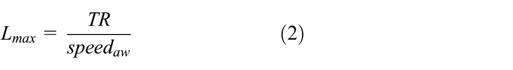
Now, we prove by contradiction that

Assume that

then

Similarly, we have

Therefore

In addition, for another MIS node v′, there exists a black path

That is, for any CDS nodes v′ and

This completes the proof.
Theorem 10 shows that the third algorithm guarantees constant approximation ratio in terms of CDS size. We first prove Lemma 6 for the proof of Theorem 10.
Lemma 6
In UDGs or UBGs, if

where
Proof
The third algorithm constructs a dominating tree with the black paths. In this dominating tree, each non-leader MIS node is connected to its parent MIS node by the shortest three-path between them. Therefore, there are at most

Theorem 10
If

and in UBGs,

where
Proof
According to Lemmas 4–6, we have that, in UDGs

and in UBGs

Theorem 11
The time complexity and message complexity of the third algorithm are
Proof
The third algorithm spends constant operations to add an MIS node to the dominating tree. Thus, the theorem holds.
Simulation
In our research, we carried out extensive simulations to test the performance of our algorithms. Among the simulation tools for USNs,
46
we use the UAN framework of the ns-3 simulator (version 3.26) in this article. The UAN framework provides a Thorp propagation model to simulate underwater acoustic communications. The simulation parameters are presented in Table 2. A 2D network is modeled as a set of nodes randomly deployed in a
Simulation parameters.

Since existing routing cost optimization CDS algorithms measure only hop-distances among nodes and their implementations are hard to be extended to edge-weighted graphs, we use the algorithm proposed by Wan et al.,13,15 which is denoted as the Size-Optimal Algorithm (SOA), hereafter, in this article, for performance comparison. The SOA has the best-known approximation ratio in UDGs following the two-phased MIS-based approaches. The SOA constructs a two-hop MIS in the first phase and generates a dominating tree in the second phase. The approximation ratio is controlled because a two-hop MIS can be connected by almost the same number of intermediate nodes.
In addition to CDS size that is used to measure the performance of a VB, two other parameters, diameter and average routing path length (ARPL), are used to evaluate the communication latency of the network. ARPL was first introduced in Kim et al., 29 which is defined as the average of all routing path lengths in the CDS. Simulation results indicate that our algorithms clearly improved the communication latency of the network with controlled VB size. The details are presented as follows.
Performance versus the number of nodes
The effects of the number of nodes in 2D networks are presented in this section. The results are shown in Figure 6. The number of nodes ranges from 100 to 500 nodes. The transmission range of nodes is fixed at 250 m. The size, diameter, and ARPL are, respectively, presented in Figure 6(a)–(c).
Performance versus the number of nodes in 2D networks. With different numbers of nodes, the performance of our algorithms is compared with SOA in terms of: (a) size of the CDS, (b) diameter of the CDS, and (c) ARPL of the CDS.
As shown in Figure 6(a), in terms of CDS size, the third algorithm and SOA perform closely, and they clearly outperform the first and the second algorithms. In addition, the CDS size of the third algorithm and SOA increases little with the number of nodes, which indicates good scalability of them in terms of CDS size. For the first algorithm, the size of the CDS increases rapidly with the number of nodes in the network. The CDS size of the second algorithm also increases clearly with the number of nodes. This is reasonable because the first algorithm guarantees no performance to CDS size and the approximation ratio of the second algorithm in terms of CDS size is large.
For CDS diameter and ARPL, as shown in Figure 6(b) and (c), the first algorithm performs the best and SOA performs the worst. The proposed algorithms in this article perform closely, and they significantly outperform the SOA. In addition, it can be seen that the diameter and ARPL of CDS do not change clearly with the number of nodes. Thus indicates that the number of nodes in the network should not affect the decision to select the CDS construction algorithm while concerning the network communication latency.
In all, the third algorithm is promising to be used for CDS construction in USNs due to its good performance on all of the size, diameter, and ARPL of CDS. However, if the number of nodes in the network is not large, the first and the second algorithm can also be concerned to be used because their performance gap to the third algorithm and SOA is not very big according to Figure 6(a). If the network manager is quite aware of the network communication latency, then SOA is not suggested to be used because it will greatly increase the network latency. In fact, a large latency means high energy consumption to achieve the communication tasks among nodes.
Performance versus transmission range
In the simulation, the effects of the transmission range to the performance of the algorithms are also tested in 2D networks, and the results are shown in Figure 7. In this section, the number of nodes in the network is fixed at 200. The transmission range is selected from 200 to 400 m.

Performance versus transmission range in 2D networks. With different transmission ranges, the performance of our algorithms is compared with SOA in terms of: (a) size of the CDS, (b) diameter of the CDS, and (c) ARPL of the CDS.
As shown in Figure 7(a), the CDS size decreases with the transmission range for all the algorithms. This is reasonable because when the transmission range increases, the network density also increases, so that less nodes are required to form a CDS. The first algorithm performs the worst for different transmission ranges. The second algorithm also does not perform well with small transmission ranges, but the performance gap between the second algorithm and the third algorithm becomes small when the transmission range increases. The third algorithm and the SOA perform well, which is reasonable because the third algorithm and the SOA achieve good approximation ratio in terms of CDS size.
For the diameter and ARPL, it can be seen that the proposed algorithms significantly outperform the SOA as shown in Figure 7(b) and (c). Although the performance gap between SOA and the proposed algorithms becomes smaller when the transmission range increases, the performance gap is still clear when the transmission range is close to 400 m.
In all, the third algorithm in this article performs well in terms of both CDS size and network latency. When the transmission range is big, the second algorithm is also a promising choice because its performance on CDS size becomes close to the third algorithm and the SOA.
The simulation results in 2D networks are in good agreement with the theoretical analyses presented before. For example, SOA guarantees the best approximation ratio in terms of CDS size, but it cannot guarantee the performance of network latency. The first algorithm and the second algorithm cannot guarantee good performance ratio in terms of CDS size, but they guarantee very good performance in terms of CDS diameter or ARPL. The third algorithm achieves a good trade-off between CDS size and latency and guarantees good performance for both CDS size and network latency.
Performance in 3D networks
The simulation results of 3D networks are presented in Figure 8. In Figure 8(a1), (a2), and (a3), we fix the transmission range at 200 m, and test the algorithm performance with different number of nodes in the network. In Figure 8(b1), (b2), and (b3), we fix the number of nodes at 200, and test the algorithm performance with different transmission ranges.
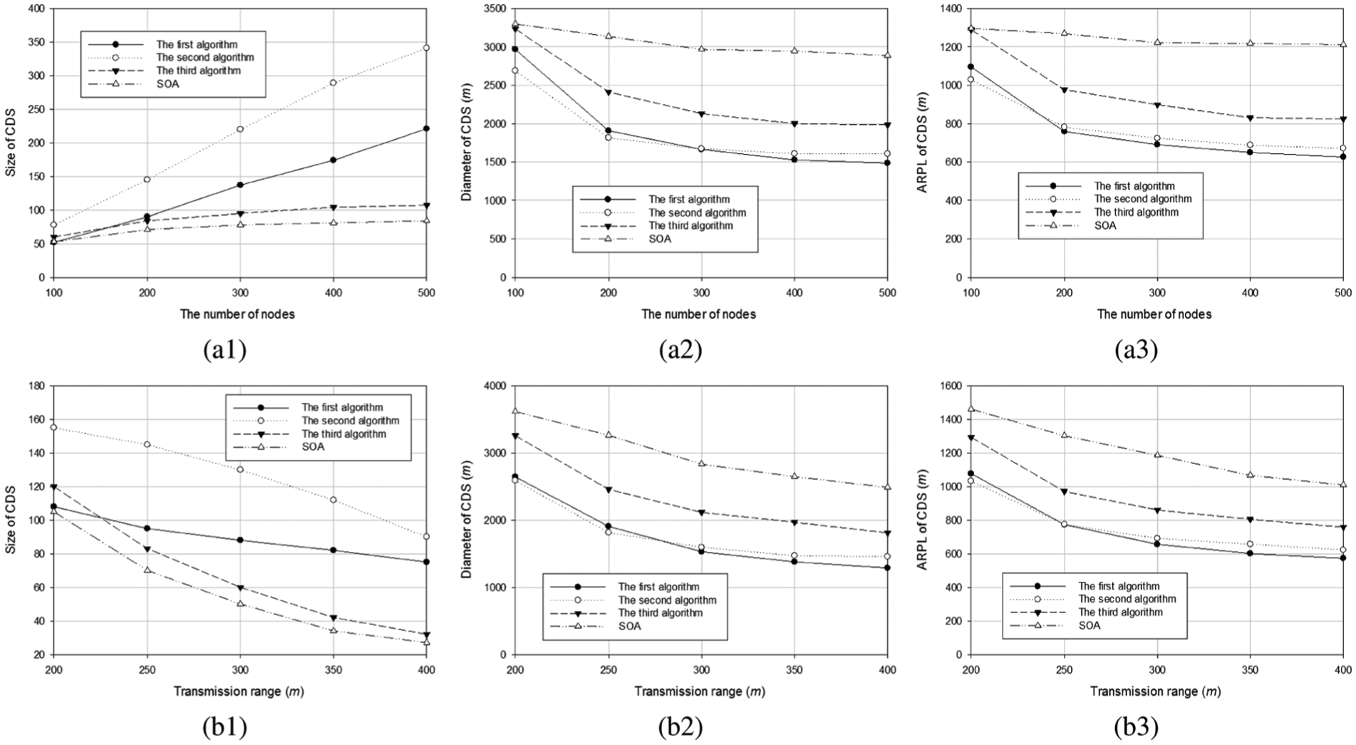
Algorithm performance in 3D networks: in (a1), (a2), and (a3), the performance of our algorithms is compared with SOA with different numbers of nodes and in (b1), (b2), and (b3), the performance of our algorithms is compared with SOA with different transmission ranges.
The simulation results of 3D networks are similar to the results of 2D networks. As shown in Figure 8, the third algorithm performs well for all size, diameter, and ARPL of the CDS. The first and the second algorithm perform well in terms of CDS diameter and ARPL, but they cannot perform well in terms of CDS size when the number of nodes or the transmission range is large. These results are also in good agreement with the theoretical analyses presented before.
Conclusion
Communication latency greatly influences the performance of USNs because of the limited propagation speed of acoustic waves. The use of VB aggravates this problem because restricting routing tasks to backbone nodes inevitably increases length of a routing path. In this article, we use the weight of an edge to represent latency between sensor nodes. A USN is abstracted as an edge-weighted graph. Under such model, we suggested to control not only size but also the routing path lengths of a CDS as a VB. Therefore, we devised three algorithms to optimize both size and routing path length of a CDS.
The first algorithm guarantees two-approximation to CDS diameter and guarantees no constant approximation to CDS size. For a pair of nodes with minimum latency
Extensive simulations have been conducted and the results show that the proposed algorithms can achieve good trade-off between the backbone size and network communication latency.
Footnotes
Handling Editor: Miguel Ardid
Declaration of conflicting interests
The author(s) declared no potential conflicts of interest with respect to the research, authorship, and/or publication of this article.
Funding
The author(s) disclosed receipt of the following financial support for the research, authorship, and/or publication of this article: This work was supported by the National Natural Science Foundation of China (NSFC) (grant nos. 61702298, 61602205, 51627805, and 61170004), National Key Research and Development Program of China (grant nos. 2016YFB0201503 and 2016YFB0701101), Specialized Research Fund for the Doctoral Program of Higher Education (20130061110052), Major Special Research Project of Science and Technology Department of Jilin Province (20160203008GX), Key Science and Technology Research Project of Science and Technology Department of Jilin Province (20140204013GX), and Graduate Innovation Fund of Jilin University.