
Abstract
Inertial navigation system needs to be initialized through the alignment process, before the transition into the navigation stage can be made. In this article, a robust cascaded strategy of alignment which aims to provide an automatic operating alignment strategy for different application scenarios is proposed. The robust cascaded strategy of alignment utilizes the advantages of several alignment methods to form a cascaded alignment strategy. As a result, the robust cascaded strategy of alignment can be utilized in applications with different grade inertial measurement units under complex dynamic condition. In addition, several control measures are added into the robust cascaded strategy of alignment process to increase its robustness and to ensure that acceptable performance may be attained. A filed test using two inertial measurement units (tactical-grade FSAS and micro-electro-mechanical-system-grade SBG) shows that the proposed robust cascaded strategy of alignment can achieve alignment under various dynamic conditions, such as low speed motion, turns, stationary positions, and straight motion. The mean heading error and level angle error are 0.10° and −0.08° for the FSAS, respectively, and −0.44° and −0.02° for the SBG, respectively. The root mean square of the heading error and level angle error for the FSAS are 2.08° and 0.50°, respectively, while those for the SBG are 2.95° and 1.44°, respectively.
Keywords
Introduction
Strapdown inertial navigation system (SINS) needs to obtain initial states through the alignment process before the transition to the navigation stage.1–3 In addition, the alignment performance will directly affect the accuracy of navigation solution. 4 The alignment usually consists of two steps: coarse alignment and fine alignment. In current research, many studies are focused on the improvement of fine alignment by modifying the error models in the Kalman filter5,6 or by applying special state estimators such as an unscented Kalman filter.7,8 These works are meaningful, but coarse alignment can always provide satisfactory results for most navigation applications. Therefore, coarse alignment is the main subject of this article.
Coarse alignment can be classified into two categories based on the dynamics of SINS upon the initialization: stationary alignment and in-motion alignment. When SINS is stationary, analytic alignment can be conducted. Stationary alignment requires gyroscopes that can sense the rotation of Earth which limits its application in low-grade inertial measurement units (IMUs) especially micro-electro-mechanical-system (MEMS) IMUs. Under these circumstances, alignment on a moving base needs to be implemented, and it is essential to integrate external aiding sources with SINS data using some form of the measurement matching method.2,7 The conventional coarse alignment methods used on a moving base can be divided into three types. The first type involves using the velocity matching method (VMM) or constructing a position vector through position solutions of two points to obtain the initial heading and using data from accelerometer to obtain level angles is a convenient way.3,9 Unlike the way of utilizing extern aid information in above-mentioned methods, Ma et al. used global positioning system (GPS) measurements to construct special vectors that are needed in solving the attitude matrix equation, similar to the analytic alignment method. This is the second type of conventional coarse alignment methods, and it yields desirable initial attitude results. 10 Another type of in-motion alignment method, known as the optimization-based method (OBM), utilizes gravity in the inertial frame as a reference and transforms the attitude method into a continuous attitude determination problem.11–13 In OBMs, the attitude matrices are decomposed to form the process model, velocity and position are integrated to construct measurements, and quaternion optimization is utilized. The OBMs can provide accurate results, but they may need a long time to converge under low dynamic conditions.
Among the aforementioned in-motion alignment methods, most can perform well under specific circumstances. However, it is difficult to find a method that can be applied to various complex conditions. With the popularization of low-cost SINS, in-motion alignment is demanded in many applications such as pedestrian dead-reckoning, robots, and self-driving vehicle. As a result, it is meaningful and essential to provide a practical, effective, and robust strategy that can be widely applied. Unfortunately, the majority of the existing research focuses on investigating only one method rather than a set of strategy of in-motion alignment. In this article, we investigated the performances of several practical algorithms and presented their inherent flaws. Then, an robust cascaded strategy of alignment (RCSA) which can be applied to complex and protean dynamic conditions is proposed based on the drawbacks of each single method.
Theories and models of alignment
In a way, stationary alignment can be treated as a special type of in-motion alignment, so it is classified as in-motion alignment in this article. Because the most commonly used aiding information for in-motion alignment is velocity and position provided by global navigation satellite system (GNSS), the in-motion alignment problem in a GNSS/SINS integrated system is taken into consideration. For other external information sources, such as the Doppler Velocity Log (DVL) and odometers, the theories and models in following discussion are still applicable.
The coordinates and nomenclature used in this article are defined as follows:
i-frame: Earth-centered inertial coordinate frame in which the x-axis points to the spring equinox and the z-axis is oriented parallel to the rotation axis of the Earth.
b-frame: Carrier body frame in which x-axis points to the right and the z-axis points up, forming the right-handed system.
e-frame: Earth Centered and Earth Fixed (ECEF) frame.
n-frame: Navigation frame, the common east-north-up local level frame.
Stationary alignment
Stationary alignment (SA) can be achieved using leveling, followed by gyro-compassing or an analytical method.
3
The analytical method utilizes gravity (

The premise of implementing SA is to detect the stationary epochs precisely. In this article, we use GNSS velocity and position results combined with the magnitudes of IMU outputs to detect stationary epochs. First, if the amplitude of GNSS velocity is less than 0.03 m/s, or the vibration of the position is less than 0.03 m during 1 s, then the epoch is treated as a stationary epoch. Second, when the GNSS velocity and position result are unavailable, the average amplitude of the gyroscope during 1 s is calculated, and a stationary epoch is detected if the average amplitude is less than a given threshold.
Velocity matching method
The VMM takes advantage of the velocity solution in the n-frame which is tightly related to the azimuth. So heading can be determined by the projection of the velocity vector in a local level plane. This principle is illustrated in Figure 1.

Heading derived from velocity.
Hence, the heading can be calculated as follows

Regarding the level angles, some literature simply sets them to zero with an uncertainty and then moves into the fine alignment stage. 15 This is practical when the level angles are small. However, it may take a long time to converge or even lead to divergence in fine alignment if the carrier is not of an approximate level. As the acceleration of the carrier in the n-frame can be derived from the navigation equation, it is possible to use accelerometer leveling to offer more accurate level angles.
The navigation equation in the n-frame is given as

where
In addition,

where

Substituting equation (5) into equation (4), the level angles can be expressed as

Some very low-cost GNSS receivers can only provide position solutions. In case like this, position-derived velocity can treated as a substitute in the above method.
Once the coarse alignment process is finished, the misalignments can be calculated through the fine alignment process if more accurate attitudes are demanded in practice. As shown in Figure 2, the Kalman filter is used to estimate the misalignments. The position and velocity for mechanization are reset by the GNSS results, while the initial attitudes are obtained from the coarse alignment process.

Flow chart of fine alignment.
Actually, fine alignment is a type of degraded loosely coupled (LC) update. On the basis of LC model in the n-frame, a reduced-state fine alignment model incorporating East and North velocity errors and attitude errors can be obtained by removing the columns and rows related to the position and the up-velocity. 15
Position vector method
In some application scenarios, the GNSS may be suspended for a few seconds because of signal blockage or logging problems. This can occur frequently when using low-cost receivers. If the time interval of the suspension is short, the position solutions at both ends of the suspension time are still reliable. In addition, the speed of an IMU under low dynamic conditions, such as the pedestrian dead reckoning (PDR), may be too low for the VMM during the whole navigation. Under this circumstance, we can use two position vectors to obtain the heading. This method is referred to as the position vector method (PVM) in this article, and its principle is illustrated in Figure 3.
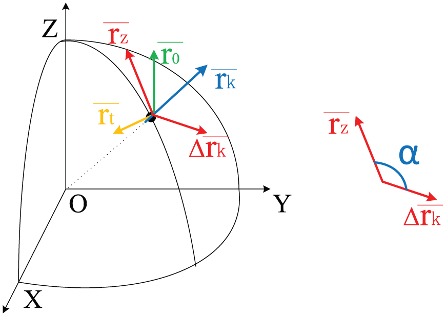
Principle of position vector method.
Let

where the dash above the vector indicates that it is a unit vector, and
Subtracting
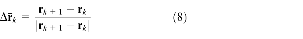
The angle between

Optimization-based method
The OBM is obtained from the alignment principle in the i-frame which can be described as follows. The OBM first attempts to filtrate the apparent acceleration and recover the gravity component in the b-frame and then conducts integration manipulations to obtain the velocity or position in the

Alignment strategy
The in-motion alignment methods discussed above can provide good results for many applications, but they may fail in certain cases, which would have serious detrimental effects on the navigation solution. Therefore, it is worthwhile to make their limitation clear and develop a robust strategy. This section will analyze the error characteristics of above methods first and then give some robust tactics. The RCSA is presented at the end.
Error analysis
It is inevitable that GNSS velocity and position results will include errors. Therefore, attitudes calculated using GNSS velocity and position will also contain errors. In addition, accelerometer and gyroscope biases will also affect alignment performance. However, by analyzing the error propagation from velocity/position errors to attitudes errors, several robust policies such as quality control and switching between different methods can be conducted. For the VMM and PVM, the heading is the main task, so only heading error will be discussed for them.
VMM
The heading error in VMM can be obtained simply by conducting differential manipulation, as shown in equation (2), and by applying the error propagation law

As we can see from equation (11), the heading standard deviation,
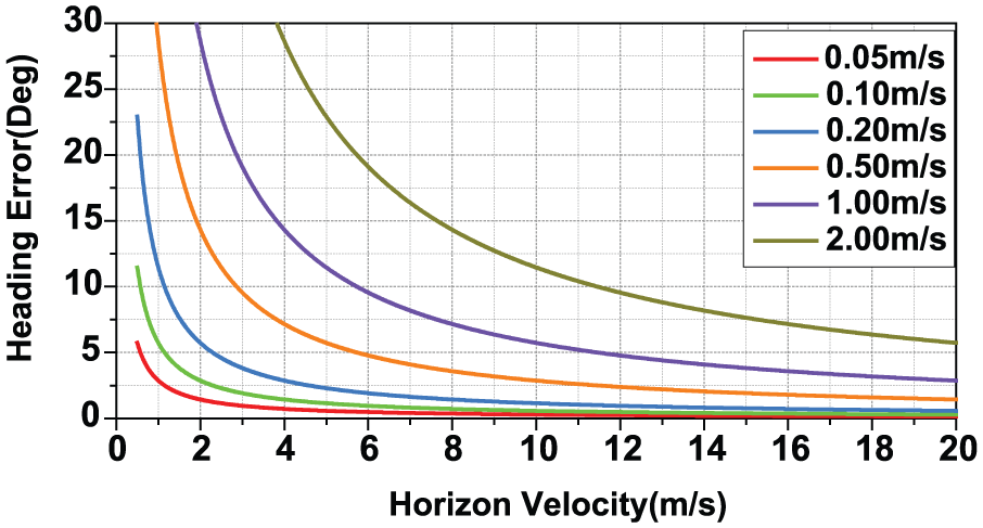
Heading errors with respect to horizon speed and standard deviation of velocity using the VMM.
Based on the above analysis, we set the requirement for utilizing the VMM. On one hand, the horizon speed needs to be greater than 2.0 m/s. On the other hand, the standard deviation of velocity should be less than 1.0 m/s.
PVM
In the PVM, the heading error is merely related to position errors at time

where the prefix,

It can be seen from equation (13) that the heading error,

Heading errors with respect to baseline length and standard deviation of position of the PVM.
OBM
When solving equation (10), the Q-method is deeply dependent on the output of the IMU. This means that the OBM is susceptible to the bias of the gyroscope and accelerometer. The literature 12 gives the relationship between attitude errors and IMU bias

where
A robust cascaded strategy of alignment
Based on the above error analysis and the performance of the OBM described in the literature, 12 the RCSA is proposed. On one hand, it can switch between different alignment methods automatically to conduct alignment successfully and accurately for different land application scenarios. On the other hand, several robust policies are added to ensure that the alignment results are reliable. The RCSA process is as follows:
Detect stationary epochs and determine whether the SA can be conducted.
The RCSA commences with the determination of whether the SINS is stationary or dynamic using the IMU data assisted by the GNSS. If the stationary time interval is larger than 60 s, the SA will be executed. Otherwise, it will move to the dynamic alignment procedure. It is worthwhile to note that there is no need to conduct stationary detection for low-grade IMUs whose gyroscopes are not capable of sensing the rotation of the Earth.
Prepare data for the VMM and PVM.
The GNSS velocity solutions will be scanned first to find the appropriate starting epoch. According to the error analysis conclusions, the horizon speed needs to be greater than 2.0 m/s and its standard deviation needs to be less than 1.0 m/s. For the VMM, we set a data window of 4 s empirically. If all data in the window meet the above requirements, then the VMM is ready to be conducted. For the PVM, GNSS position solutions are used. The standard deviation of position should be less than 1.0 m, and the length of the baseline needs to be longer than 8.0 m.
Actually, what we obtain using the VMM and PVM is course over ground (COG), rather than heading. For marine and aviation applications, the difference between COG and heading causing by lateral wind or ocean currents sometimes cannot be negligible. For land application such as vehicle navigation and PDR, the difference is very small. Because this article is focused on the land scenarios, it is rational to substitute COG in place of heading. However, one thing that should be noted is that the COG differs from heading, even in land scenarios, when the vehicle is turning during the alignment process. Therefore, it is essential to determine whether the track of the data for alignment is relatively straight, especially when using the PVM. The outputs of the z-axis gyroscope during the time window are used to check the track. The procedure is represented as
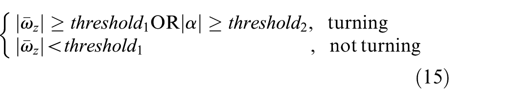
where
Execute the VMM; if the VMM is successful, the alignment is complete.
The first epoch in the data window for the VMM is used to calculate the attitude and heading error. If the heading error is less than 15.0°, the determined attitude is used to initialize the fine alignment as shown in Figure 2. After 4 s of mechanization, the terminal attitude can be obtained by compensating misalignments output from the Kalman filter to the mechanization attitude.
Execute the PVM; if PVM is successful, the alignment is complete.
The PVM will be executed if the VMM fails and the data for the PVM are ready. The level angles in the PVM can be obtained through the accelerometer leveling, under the premise that there is no external acceleration, except for the gravity. This hypothesis is rational for most land applications.
Execute OBM and the alignment finished.
The OBM will be implemented under conditions where neither the VMM nor the PVM can provide a reliable result. This method usually requires dozens of seconds to converge for land applications, which is the main reason why it is ranked after the VMM and PVM in the RCSA. In addition, the OBM can perform well even when the IMU experiences a strong dynamic maneuver, such as a sharp turn and this fills the gap of the RCSA.
The structure of the RCSA is presented in the flowchart, as shown in Figure 6. For simplification, the abbreviation “FA” which represents fine alignment is used in the flowchart.

Flow chart of the RCSA.
Test and discussions
Data set
The data used to verify the RCSA were collected using two types of IMUs: SPAN-FSAS and Ellipse-SBG-N. The SPAN-FSAS is a tactical-grade IMU and the Ellipse-SBG-N is a typical MEMS-grade IMU. Table 1 lists the main parameters of the two IMUs. The sample rate of the FSAS and the SBG are set at 200 and 100 Hz, respectively. A NovAtel’s SPAN receiver was used as the rover and another NovAtel receiver was operated as a base station. The baseline is less than 1 km in length and both the rover and base station have a good observation condition. Figure 7 presents the number of visible satellites and positional dilution of precision (PDOP). The average number of visible satellites and the average PDOP are 7 and 1.9, respectively. All ambiguities are fixed, which means that a very precise position solution can be obtained. The entire data collection process lasts approximately 1.5 h. The combined smoothed tightly coupled (TC) solution of FSAS provided by Inertial Explorer (IE) 8.70 is treated as the reference.
Main technical parameters of the two IMUs.


Trajectory (left), number of visible satellites (NSAT) and PDOP (right-up), and horizon speed (right-down).
In order to allow the IMUs experience more types of maneuvers as often as possible, the trajectory of the dataset includes straight lines, s-shaped turns, large circles, and squares. Furthermore, the horizon speeds of the cart are controlled to approximately 2.0 m/s most of the time. Figure 7 depicts the trajectory and horizon speed.
Results and discussions
Alignments beginning at every epoch of the dataset are conducted to test the robustness of the RCSA. Because the time costs of different alignment methods are different, the alignment results are counted to the beginning of each epoch for convenience.
Figure 8 provides the alignment results of the FSAS and the SBG IMUs. The color band at the bottom of each picture indicates which method is the applied at each epoch. As shown in the figure, alignments can be conducted successfully beginning at every epoch. For FSAS, heading errors are less than 8.0°, while pitch errors and roll errors are less than 3.0°. The maximum heading error for SBG reaches 14.0°, which is slightly larger than that of the FSAS. As the level angles for the VMM and PVM are mostly determined by the accelerometer, the pitch errors and roll errors for SBG fluctuate more violently, and its maximum level angle errors are approximately 5.0°.
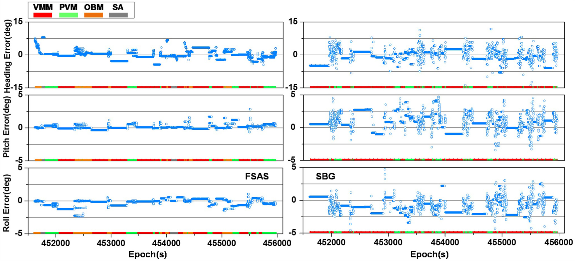
Heading errors (first row), pitching errors (second row), and roll errors (third row) of FSAS (left) and SBG (right) using RCSA.
Table 2 lists the statistical results of the four applied methods. The mean and root mean square (RMS) of the heading, pitch, and roll errors for FSAS are (0.10°, 0.16°, −0.24°) and (2.08°, 0.41°, 0.58°), respectively, while those for SBG are (–0.44°, 0.81°, −0.85°) and (2.95°, 1.46°, 1.42°), respectively. According to the test results, the RCSA can achieve alignment under complex dynamic conditions for both IMUs of different grades. In addition, the performance is considerable, meaning that it is both robust and practical. The availability of each method of the RCSA is also given in above table and the VMM plays the major role in the RCSA for both IMUs.
Maximum value (Max), Mean, and root mean square (RMS) of attitude errors using different methods (°).
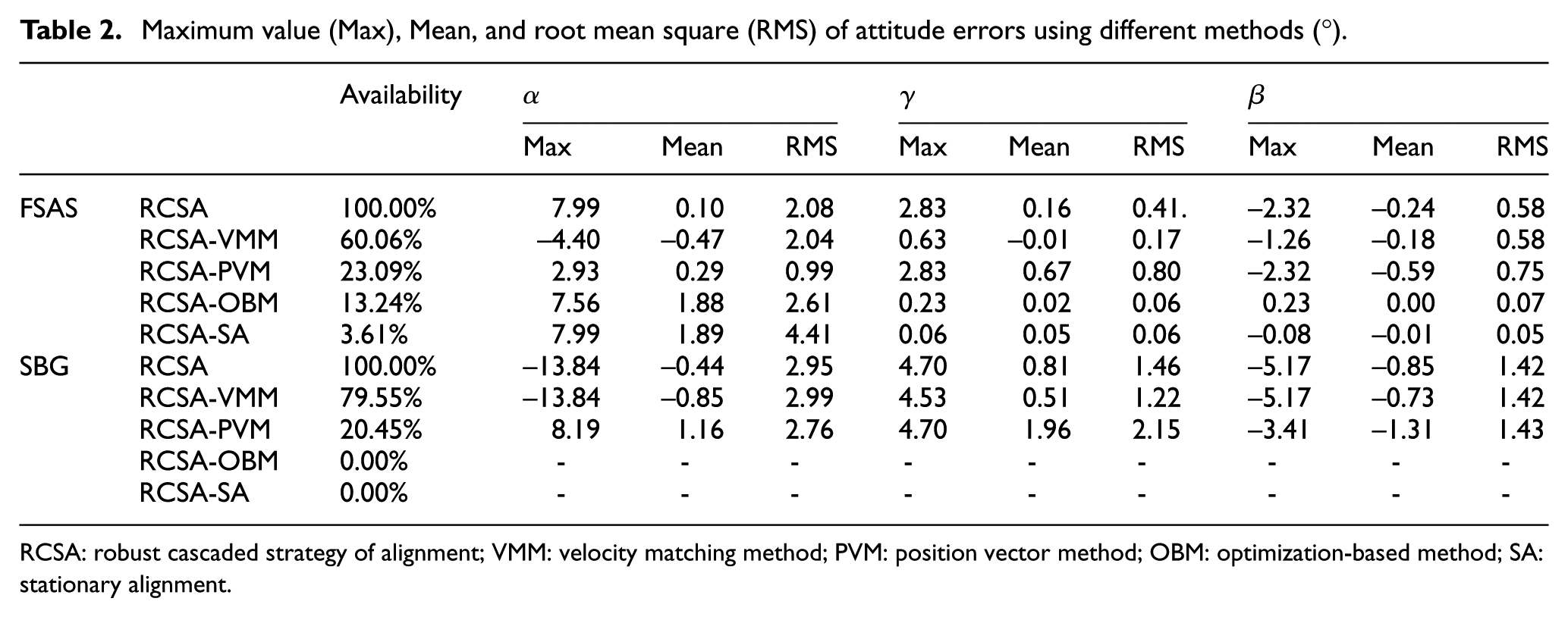
RCSA: robust cascaded strategy of alignment; VMM: velocity matching method; PVM: position vector method; OBM: optimization-based method; SA: stationary alignment.
Another phenomenon of note is that both the SA and the OBM are not used in the RCSA for the SBG. For the SA, the reason is given in the previous section. Considering the error analysis for the OBM in the “Error analysis” section, and referencing the technical parameters in Table 1, the attitude errors can be calculated roughly. For the SBG, the attitude errors may exceed tens of degrees. Figure 9 provides the attitude errors using a strategy consists of the OBM, VMM, and PVM in the alignment of SBG. As we can see from the figure, the heading error may reach approximately 70.0°, which is unacceptable for alignment. Level angle errors can exceed 30.0°. Based on the experimental results, OBM is eliminated from the RCSA for MEMS-grade IMU.

Attitude errors using the OBM in conjunction with the VMM and PVM in alignment of the SBG.
From the “Error analysis” section, we know that the heading accuracy of the VMM is related to velocity accuracy, and that of PVM is related to position accuracy. White noises are added to the smoothed TC solution of IE to test the performance of the VMM and PVM under different noise levels. For the VMM, the simulated standard deviations are 0.05, 0.1, 0.2, 0.5, 1.0, and 2.0 m/s. For the PVM, the simulated standard deviations are 0.1, 0.2, 0.5, and 1.0 m. A straight track segment of the data is selected and all horizon speeds are greater than 2.0 m/s during the selected time. Alignments are conducted beginning at every epoch. All control measures are maintained except for the constraints of the accuracy of position and velocity.
Figure 10 shows the heading errors with simulated horizon speed errors using the VMM and with simulated position errors using the PVM. Obviously, a larger speed/position error leads to larger heading errors. As the horizon speed is relatively low, the speed error at 0.5 m/s can cause a heading error at more than 10.0°. This corresponds to equation (11). For speed errors at 1.0 and 2.0 m/s, the relative error reaches 50% or larger, which can cause the heading errors to be hundreds of degrees. The performance of the PVM exhibits a similar trend, and position errors below 0.5 m can provide acceptable results.

Heading errors with simulated horizon speed errors using VMM (left) and with simulated position errors using PVM (right).
As discussed in the “Alignment strategy” section, it is essential to determine whether the track of the data for alignment is relatively straight. To analyze the influence of this step, a specific data segment is selected and the trajectory is given in Figure 11. The horizon speeds are greater than 2.0 m/s during this segment. And the smoothed TC solution of the IE is used to dilute the impact of position/speed noise.
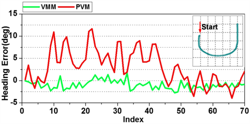
Heading errors of alignment using VMM (green line) and PVM (red line) and trajectory (right corner) of data.
The trajectory in above figure starts with a very slight bend, followed by an obvious curve, and ends with a fairly straight section. Based on previous discussions (section “Alignment strategy”), a prediction can be made that heading errors of alignment beginning at middle of the dataset may be larger than those beginning at either end of the dataset. From the test results, it can be found that heading errors of PVM experience a similar trend as predicted, but the results of VMM are not as conspicuous. This contributes to the difference between direction of horizon velocity vector and heading is tiny for land cart. Besides, the heading is determined using the instantaneous velocity and this is the biggest difference with the PVM. In the PVM, accumulated displacements are used to construct position vector and the length of the position vector needs to be long enough to decrease the percentage of position noise. So the heading at the last epoch of the alignment epoch is actually the average heading during the alignment time. As a result, any slight bend during the time interval of the PVM can cause a large heading error. Based on the different impacts on the PVM and VMM, the threshold in formula (15) may be exaggerated five times or even more.
Conclusion
Most of the existing literature related to in-motion alignment of SINS always focus on the innovation or the improvement of a single alignment method that can only perform well under specific conditions. These conditions include the use of high-grade IMU, or high-speed scenarios. In this article, we propose an RCSA for SINS that can perform well for different grades of IMUs under complex dynamic conditions. First, theories of four types of alignment methods (SA, VMM, PVM, and OBM) are introduced, and then the error formulas of the VMM and PVM are derived. Based on the derivation, the restrictions are listed as follows: (a) the two methods can perform well only while the track is relatively straight, but the requirement of the PVM is stricter; (b) the position/speed error needs to be small enough; (c) the value of speed in the VMM and the length of position vector should be large enough. According to the restrictions, the RCSA implements the four methods (SA, VMM, PVM, and OBM) with control measures one by one (in the order in last bracket). Once any method is successful, the alignment completed. The field tests using the FSAS and SBG show that the RCSA can achieve alignment beginning at any epoch in the dataset. Furthermore, a conclusion that the OBM cannot be used for low-grade IMU (such as MEMS IMU) is obtained through theoretical and experimental analysis.
Benefitting from the strict control measures, the RCSA can provide robust alignment solutions for SINS ranging from high-grade SINS to MEMS-grade equipment. The RCSA is practical and valuable and can be applied in many applications equipped with an IMU, such as vehicle applications and PDR.
Footnotes
Academic Editor: Hassen Fourati
Declaration of conflicting interests
The author(s) declared no potential conflicts of interest with respect to the research, authorship, and/or publication of this article.
Funding
The author(s) disclosed receipt of the following financial support for the research, authorship, and/or publication of this article: This work is supported by the National Key Research and Development Program of China (no. 2016YFB0501803) and the National Nature Science Foundation of China (no. 91638203).