Deep learning–based real-time query processing for wireless sensor network

Abstract

The data collected from wireless sensor network indicate the system status, the environment status, or the health condition of human being, and we can use the wireless sensor network data to carry out appropriate work by processing it. In recent years, using deep learning, it is possible to construct a more intelligent context-aware system by predicting future situations as well as monitoring the current state. In this article, we propose a monitoring framework for wireless sensor network streaming data analysis based on deep learning. In particular, in an environment where time requirements are strictly enforced, data analysis results must be derived within a deterministic time. Therefore, we conduct query refinement adaptively to enable timely analysis of wireless sensor network data in the predictor. Even if some sensor data that is not synchronized in time are included or even if some data have not arrived yet, reasonably accurate query analysis results can be obtained within the deadline by performing the proposed method.

Keywords

Wireless sensor network query processing deep learning real-time system monitoring

Introduction

Wireless sensor network (WSN) data are the result of measuring the available values from the physical environment. Sensor data are already widely used in everyday life. The types of data that can be obtained from the sensors are temperature, brightness, motion, chemical values, and biological signals. These data can be used to observe human health conditions, system conditions, or environmental information. It can also continuously monitor the data coming from the sensor, and if the sensor value satisfies a certain condition or goes out of the reference value, it can handle the appropriate task corresponding to the situation.

With the rapid enhancement of hardware in recent years, the WSN environment becomes more complex and more versatile. Munir et al.¹ proposed a WSN architecture composed of nodes with multi-core, and the data collected in this environment can handle high-level applications compared to the past. As the quality of sensor data is improving, researches are being conducted to analyze WSN data by machine learning. Machine learning is a technique for analyzing the meaning of new data based on the history of past data. In the case of streaming sensor data, data can be collected and stored continuously; therefore, we can analyze and monitor sensor data using various machine learning techniques like classification or regression. Alsheikh et al.² presented machine learning studies related to WSN that various machine learning algorithms are applicable to WSN because WSN covers a very wide range of information and communication technology (ICT) applications. Especially, the high level of machine learning represented by deep learning shows fairly accurate classification and prediction performance. Thus, when new WSN data arrive, we can predict what the system will potentially be concerned with the ICT domain.

However, in an environment where temporal processing is important, it may be difficult to stably analyze the streaming sensor data. For machine learning analysis, it is necessary to construct several sensor data as one feature vector. Also, the feature vector should consist of data of the same time window. In an environment like WSN, data may not arrive within a definite time or may be imprecise due to problems such as network delay, hardware limitations of device, and complex natures of the surroundings.³ In this case, if we wait for the data to use the completed vector, it will not be able to produce the analysis results within the deadline, and we will not get the results available in time-critical environments. On the other hand, if the analysis is performed without considering the missing data, the results can be obtained within a definite time, but the accuracy of the analysis is low and the monitoring stability can be deteriorated.

In this article, we propose a query processing system for analyzing streaming sensor data collected from WSN. Especially, we design real-time monitor which can perform deep learning–based analysis within the deadline considering time-constrained environment. Simulation using the published data and the performance of the deep learning under time constraint are reported and discussed to assure the effect of the proposed technique.

Query processing framework for analyzing sensor data

Overview

In WSN system, the base station, a powerful server outside of the WSN, collects sensor data and processes the data to utilize them.⁴ In addition, it monitors the overall situation. Our approach is to equip a deep learning analyzer into the base station so as to provide useful analysis results. The overall process flow of sensor data collection, deep learning analysis, and results reporting is shown in Figure 1.

Figure 1.

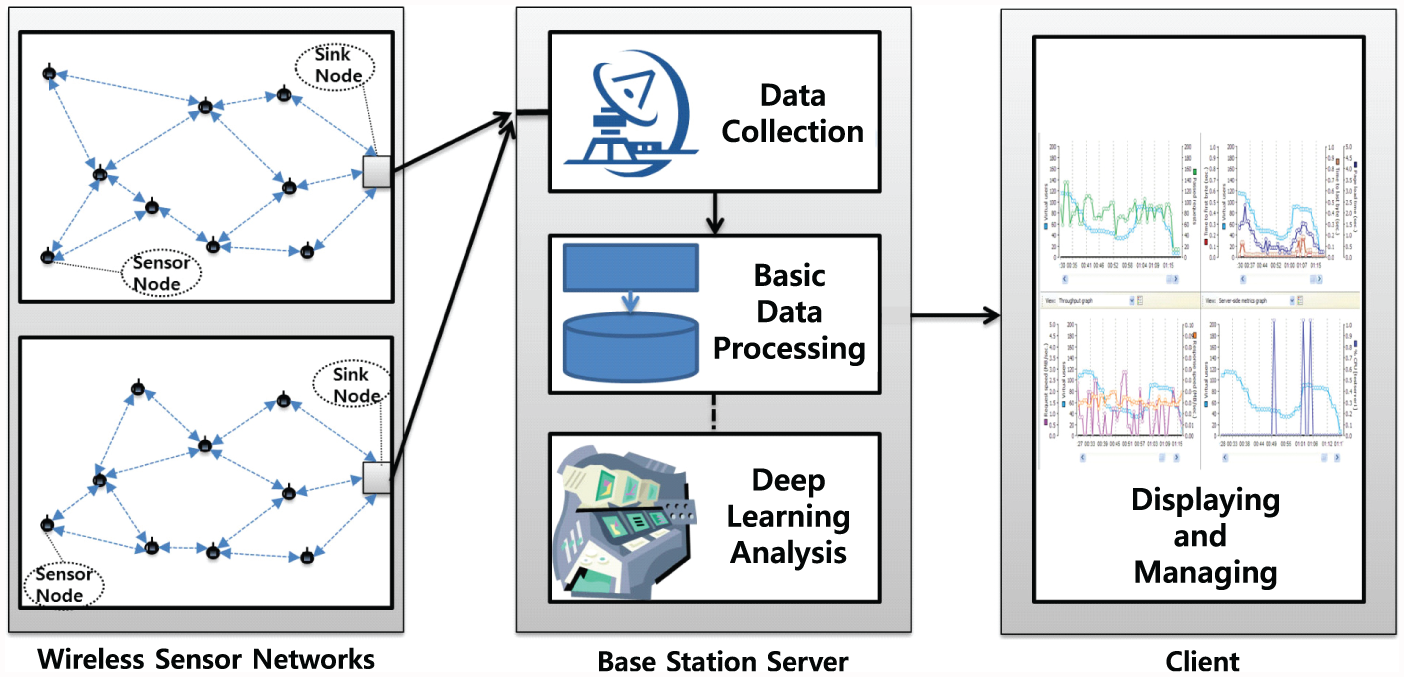
Overview of WSN data processing framework.

As shown in Figure 1, the distributed WSN nodes transmit data to the base station server via the main sink node. The base station server collects data and performs basic processing. The collected data are stored in a database, the sensor measurement value is checked to identify whether the measured value satisfies a specific constraint condition, and the result is informed to the user. In addition, the proposed method queries the data to the deep learning analyzer to perform in-depth analysis of the current situation. For example, even though the individual sensor values do not exceed the constraints and seem to be unproblematic, the deep learning analyzer can produce a prediction that it is in a state of danger when comprehensively assessed. The predicted information is used to trigger the appropriate actions or be delivered to the user.

Architecture design

The architecture of the base station server is shown in Figure 2. In the figure, the solid rectangle represents the module, and the dotted rectangle represents the decomposition of logical function. The following is a description of the major modules.

Figure 2.

Architecture of the proposed base station monitor.

Streaming data collector

The Streaming Data Collector plays a fundamental role in collecting streaming data from each WSN. The collected data are stored in the database. It also sends the data to the deep learning processor or to the monitoring condition checker.

Deep learning model generator

In order to perform deep learning, a training model must be created in advance. The Deep Learning Model Generator performs machine learning using stored sensor data. In fact, deep learning algorithms are very diverse, such as convolutional neural network (CNN), recursive neural network (RNN), long short-term memory (LSTM), and deep belief network (DBN), and have different advantages depending on the data characteristics. Therefore, this module applies a deep learning technique suitable for domain characteristics. The created deep learning model is delivered to the Deep Learning Predictor. Data training and model generation are computationally expensive and time-consuming tasks, so it is desirable to perform them every few days or every few weeks by a scheduler.

Deep learning query generator

The data acquired from the sensor needs to be generated as a query for deep learning analysis. The query is the result of constructing each sensor data into a feature vector. The query generator holds the recently arrived data in the temporary memory database and constructs the feature vector at the point where the deep learning query is to be executed. In order to construct the values of several heterogeneous sensors into one feature vector, it needs to be synchronized with time. Therefore, the value of each sensor data is extracted based on a time window of a predetermined size and is generated as a query. However, since certain feature values may be imprecise depending on the situation, we perform query refinement to compensate for this. The completed query is sent to the Query Processor. Note that the Query Generator, Query Refinement, and Query Processor components are real-time tasks. These tasks are executed with a high priority, unlike other common tasks, and are not preempted by other low-priority tasks. This requires a real-time system such as a real-time OS or Real-Time Specification for Java (RTSJ).

Query processor

The Query Processor is responsible for requesting the Deep Learning Predictor for query analysis and receiving the results. It communicates with the Deep Learning Predictor through real-time queues and operates in soft real time. The time information of the events together with the query processing result is sent to the Monitoring Condition Checker to check whether the result of the response satisfies the time constraint.

Deep learning predictor

The Deep Learning Predictor uses the query as input and returns the result. The result is derived from classification or regression method. Classification is to predict the input query is classified to which kind and regression is a technique to deduce the value of a specific factor from the input query. We can apply various machine learning models depending on the situation.

Monitoring condition checker

The basic roles of the base station server are to check the value of the sensor data, to grasp the current situation, to respond appropriately, and to notify the manager. The Monitoring Condition Checker performs monitoring function to check pre-set condition continuously. The Data Checker is a component that determines if the measured value of the sensor meets the valid condition. It is therefore used to trigger direct actions based on the results of the checkers. In contrast, the Prediction Result Checker identifies the results of the deep learning analysis. Because prediction represents potential situation, unlike direct data, it can be used as a guide to flexibly coping with situations rather than responding strongly. Meanwhile, in a time-constrained environment, it is important to monitor to ensure whether timing violations occur or not, as they can cause harm to people, money, or the system. Therefore, the Timing Correlation Monitor component plays a role of monitoring whether the deep learning task satisfies pre-defined time constraints.

Deep learning analysis

In this study, we use deep learning which shows good performance in recent data processing among machine learning methods.⁵ Deep learning was introduced in the 1980s, but it was not well used for problems such as local optimal convergence problems and excessive computation. As learning algorithms improve and hardware performance improves, they are attracting attention again. Deep learning is most notable because it shows higher accuracy than previously known machine learning algorithms. Currently, our architecture is designed to use deep learning techniques; however, it can be easily integrated with other machine learning algorithms requiring less computation power depending on the situation. The deep learning technique described in this section is the CNN (Convolutional Neural Network; UFLDL Tutorial, http://ufldl.stanford.edu/tutorial/supervised/ConvolutionalNeuralNetwork/) model designed for our case study.

Figure 3 shows the architecture of the CNN model for learning sensor data. The major steps of learning process in the proposed model are summarized as follows:

In the first convolution layer step, 200 convolution filters of 3 × 3 size are used. In our experimental environment, there are 72 features. The convolution filter extracts 3 × 3 convolution features from 8 × 9 input data and collects data from 200 filters in different ways. The size and number of filters can affect the analysis depending on factors such as the size, type, and complexity of the data. Therefore, we determined the values that show good performance through experiments.

In the convolution feature extracted from the convolution layer, a characteristic value is selected through a max-pooling process. Max-pooling is one of the pooling techniques that selects the largest value in a given feature. Max-pooling results are merged into one.

The proposed model consists of two stages of convolution and max-pooling. Then, we apply softmax regression (Softmax Regression; UFLDL Tutorial, http://ufldl.stanford.edu/tutorial/supervised/SoftmaxRegression/) to the pooled features to obtain the probability of belonging to each class. It is classified as a class having the highest probability.

The values of the convolution layer and the softmax regression matrix can be modified by backpropagation technique when the classification test is not matched with the ground truth. This process corrects the classification performance.

In CNN, internal values such as convolution layer can converge abnormally in order to increase the accuracy in specific input (learning data) as learning progresses. In this case, the training data show high accuracy but the test data can show low accuracy. To solve this problem, dropout is applied to prevent overfitting in deep learning.

Figure 3.

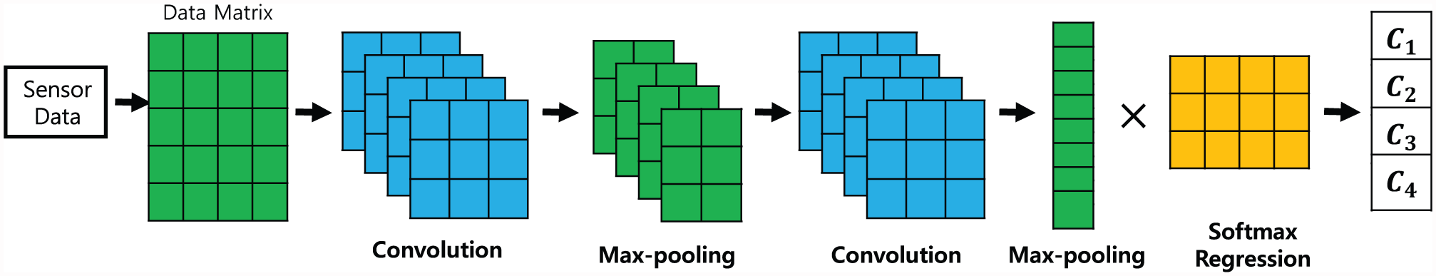
CNN model architecture used in our deep learning engine.

The prediction process is also very similar to the learning process described above. The above three steps (1–3) are the same as the prediction method.

Deep learning analysis of sensor data in real-time system

Guaranteeing timing constraints for streaming sensor data analysis

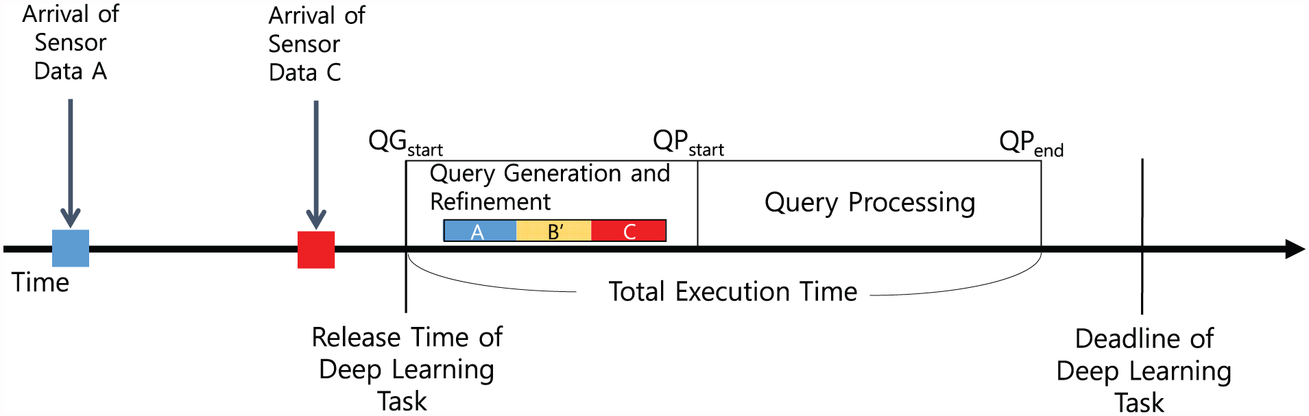
We focus on real-time processing of deep learning. In time-critical environment such as cruise control, online stock trade, and medical device, since violation of time constraints can cause great disaster, specification for timing constraints and its monitoring are very important. In a real-time system, task processing must be deterministic, and operating system capable of priority-based task scheduling is essential. However, it is not a complete real-time system that only a high-priority task is not preempted by another task. It is more important that the task finishes execution within the deadline and must be guaranteed when the time constraint is hard-real-time. In this section, we present how our framework guarantees timing constraints in streaming sensor data analysis. Figure 4(a) shows the process of collecting various sensor data from WSN and analyzing them in deadline time.

Figure 4.

Example for temporal processing of sensor data: (a) normal processing example and (b) deadline missed example.

First, the horizontal axis of the figure represents the time, and three types of sensor values A, B, and C are being collected by the base station over time. Using these data, the deep learning task performs analysis periodically. We assume a real-time system, so deep learning task has constraint that must be completed between release time and deadline. This task combines the collected sensor data to generate a query and inputs the query into a deep learning analyzer for query processing.

However, sensor data may not always be fully collected due to network delays or differences in sampling period. Figure 4(b) shows a situation where data B arrives late. Deep learning task tries to perform query generation after release time but pending due to missing data. After B arrives, the query is completed and analysis is performed. However, when the execution is completed, the deadline is missed and the real-time constraint is not satisfied. We therefore propose a query refinement to solve this problem. Figure 5 is an example of the proposed technique. In this example, the deep learning task starts without sensor data B like previous Figure 4(b). If there is missing data, we perform the query refinement to derive the expected B′ based on the recent history record and complete the query. After the normal query processing is performed, analysis results can be obtained within the deadline.

Figure 5.

Proposed method for temporal processing of streaming sensor data.

A specification using Real-Time Logic (RTL)-like expressions⁶ is used to model timing constraints formally and manage this process. Lee and Lee⁷ have performed real-time event detection using temporal correlation logic. Using the RTL-like expression, the following temporal logic can be expressed:

@(evA, 1) : timestamp of the first evA event instance;

@(evA, 1) + 5 ≥ @(evA, 2) : the second evA should occur within 5 time units since the first evA occurred (deadline constraint).

We specify RTL-like expressions for release events of deep learning tasks, query generation start and end events, and query processing start and end events:

@(T_release, n) : time at the n_th release of the deep learning task;

@(QG_start, n) : start time of the query generation at the n_th period;

@(QG_end, n) : end time of the query generation at the n_th period;

@(QP_start, n) : start time of the query processing at the n_th period;

@(QP_end, n) : end time of the query processing at the n_th period.

The deadline constraint can be expressed as:

@(T_release, n) + T_deadline ≥ @(T_release, n + 1)

where T_deadline is a constant value meaning deadline, which depends on the system situation. T_deadline always satisfies the following:

@(QP_end, n) − @(T_release, n) ≤ T_deadline ≤ @(T_release, n + 1) − @(T_release, n)

On the other hand, the deep learning query processing is always performed at a deterministic time because the feature set of the same size is always used, while the execution time of the query refinement may be variable depending on the situation of the arrival data. Next statement shows delay time constraint.

@(QP_start, n) − T_delay ≥ @(QG_start, n)

The real-time logic checker constantly monitors these conditions to ensure satisfaction of temporal constraints.

Query refinement

The streaming sensor data may be missing in some situations or may not be synchronized in time. Therefore, we perform refinement of inaccurate sensor data in order to reliably execute the deep learning query. Refinement of the query means complementing some inaccurate sensor data to generate a complete feature vector. The following is a process for refining a query:

Collect sensor data within the time window to be analyzed.

Identify missing sensor data.

Exponential smoothing is performed to estimate the missing sensor value(s).

Complete the query and send it to the deep learning predictor.

The exponential smoothing used in this article is also known as an exponentially weighted moving average (EWMA⁸)

s_{t} = α \times x_{t} + (1 - α) \times s_{t - 1}

(1)

where 0 < α < 1. In the equation, t indicates the current time, s_t represents estimation value of what the next value of x will be, and α is smoothing factor. Large value of α gives greater weight to recent data. In other words, EWMA is a statistical method for estimating the next data value using the sequence of observations. While EWMA is simple and easy to understand, it is argued that accuracy is reduced when the data are not linear, and the criteria for determining the value of the target range are ambiguous. Sensor data show that data changes gradually as the sampling period becomes shorter, whereas data continuity decreases when the sampling frequency is lower. Therefore, the query refinement by the moving average method depends on the characteristics of the data. In fact, we can consider other algorithms with high accuracy for refining queries, but we have chosen a simple algorithm that does not require heavy computation in consideration of time constraints. We report through the case study in the next section how there is a difference in the deep learning results applying the query refinement compared to when the actual correct values were used.

Case study

Experiment settings

For the case study, we performed deep learning analysis using sensor data sets. The case study is a simple simulation of the proposed technique exploiting CNN. The settings for CNN followed the settings described in the previous Deep learning analysis section. The data are gas sensor data published by Vergara et al.,⁹ which can be retrieved from UCI Machine Learning Repository (Gas sensor data; UCI Machine Learning Repository, http://archive.ics.uci.edu/ml/datasets/Gas+sensor+arrays+in+open+sampling+settings). These are the data of air pollution degree in a tunnel using 72 metal-oxide gas sensors. In addition, air purifying fan speed information according to the degree of air pollution is included. The purpose of the query processing in the experiment is to determine the optimal fan speed for air purification in the tunnel by analyzing the degree of pollution of the air. In fact, gas data analysis is a simple regression problem, but our purpose is to demonstrate that our architecture is general enough to integrate with various machine learning algorithms including deep learning techniques. CNN is a well-known deep learning technique with high performance in various problems such as image classifications and sentence categorizations. The example can be further extended to complex sensor data and context-aware systems such as cruise control system, intelligent traffic system, and disaster warning system.

Table 1 shows the data set information used in our experiments. There are 72 gas sensor data, and each sensor is used as a feature to construct a vector composed of 72 features. The value of the feature is an integer value representing the air gas value. We used 1,349,470 records using information acquired over time, and each feature vector has a fan speed as a class. The fan speed was defined as 30 classes by setting the range. In the case of deep learning, it is necessary to repeat training to reach a certain level of prediction accuracy. The prediction level was stabilized through 50 training iterations. Based on these models, we measured how accurately the fan speed was predicted when a new query was entered. The base station server used in the experiment was running on INTEL i7 4770 CPU, 16 GB RAM, NVIDIA gtx1080 GPU, and 8 GB VRAM. The module for CNN processing was implemented with python language and tensorflow library. The training took about 1.8 h.

Table 1.

Data set and experiment setting.

Records	Features	Classes	Iterations	Training time (h)
1,349,470	72	30	50	1.8

Experiments were performed on the query processing every 1 s period and set to 1 s for the deadline as a time constraint. We set the number of queries to 1000 each time, and the accuracy of prediction was analyzed by missing one sensor data every cycle. The purpose of the analysis is to predict the appropriate air cleaning fan speed according to the degree of air pollution. The ratio of the correct prediction is expressed as accuracy.

Experiment result

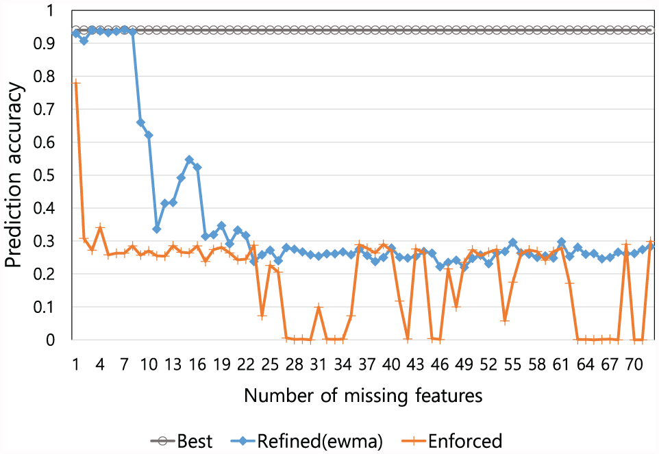
Table 2 and Figure 6 show the prediction accuracy of the experiment. In the table, Missing data is the number of sensors missing for the experiment. Refined is the result of performing the query processing after correcting the missing feature with the EWMA method, and Enforced is the result of performing the prediction by setting 0 for the feature that does not have the value. The range of recent data for EWMA was set to 100.

Table 2.

Prediction accuracy for missing data growth.

# of Missing data	Refined	Enforced
0	0.940	0.940
1	0.930	0.779
2	0.907	0.308
3	0.940	0.272
4	0.937	0.341
5	0.932	0.258
6	0.936	0.263
7	0.941	0.263
8	0.934	0.285
9	0.660	0.257
10	0.621	0.270
⋮	⋮	⋮
71	0.274	0.002
72	0.283	0.299

Figure 6.

Prediction accuracy for missing data growth.

The prediction accuracy is very high as 0.94 when all sensor data arrive normally. In the case of Enforced, accuracy is worsening to 0.3 even in the absence of two sensor values. However, in Refined case, the accuracy of prediction is rarely reduced. The prediction accuracy exceeds 0.9 even when there are eight missing data. This is because the estimated value compensates for the missing data and operates similarly to the actual data. Moreover, there is no task pending for waiting for the missing data. However, since the method of estimating the missing data is not perfect, significant data loss may lead to poor prediction accuracy. As shown in Figure 6, when more than 10 of the 72 features start to miss, the accuracy drops sharply, and in the case of missing 20 or more data, the prediction function is lost. Through the experiment, we observed that the proposed method has some limitation but shows good performance at a reasonable level.

Also, some features may have stronger prediction power than others. This means that the accuracy can be significantly reduced if a feature that has a large impact on predictive performance is missing. In order to confirm this, we experimented how the prediction accuracy changes by missing each feature one by one. Figure 7 shows the prediction result when one feature is missing. The X-axis is the 72 features aligned in order of the importance, and the Y-axis is the prediction accuracy when there is no such feature. Enforced is a naive way to predict when the feature is missing, and Refined is the proposed technique using EWMA. As shown in Enforced, in the case of a feature with a high importance, it can be seen that the prediction accuracy is greatly degraded by omission of only one feature. On the other hand, if the same feature is processed by Refined method, accuracy is significantly improved. However, there is no consistent pattern of degree of improvement, which is likely to vary depending on the data. Our experimental data show that accuracy is improved from about 0.6 to 0.9 for high-importance features.

Figure 7.

Prediction power of features.

We also measured the time spent in actual query processing. Table 3 shows the query processing time for 10 rounds. Each round is configured to process 1000 queries at once. Time on CPU means the task execution time using the CPU in the normal situation and Time on GPU is the result of performing the task using the GPU which has a superior effect on the improvement of the deep learning performance. The query generation time is not shown in this table, but it takes less than 1 ms on average to perform query generation and refinement. The average processing time for 1000 queries is about 355 ms, which shows similar results every round. In addition, query processing on the GPU has been found to be very good. Since we set the deadline to 1 s, we did not detect any violation in the Timing Correlation Monitor module because there was no deadline miss. As a result, we can confirm that it is possible to perform the deep learning process of the streaming data with a definite time.

Table 3.

Query processing time.

Round	Time on CPU (ms)	Time on GPU (ms)
1	353.90	10.11
2	348.17	10.10
3	363.01	11.06
4	356.94	11.10
5	359.00	11.12
6	353.84	11.11
7	352.28	10.17
8	348.95	11.09
9	349.82	10.67
10	367.92	10.61

Related work

WSN moves toward our daily lives such as smart office and smart home. ¹⁰ However, today’s advanced ICT environment requires intelligent WSN techniques more and more. In this regard, the convergence of WSN and machine learning is very active.

Alsheikh et al.² categorized machine learning as a way to contribute to WSN’s functional issues and how to improve non-functional requirements such as performance. Functional issues for machine learning include network routing, node clustering, data aggregation, event detection, and query processing. For non-functionality, it can be used for security, anomaly intrusion detection, quality of service, data integrity, and fault detection. Among them, our research is related to query processing and event detection.

Conventional WSN query processing was in directing tasks by checking that collected sensor data met certain conditions. However, machine learning–based query processing has been emerged to handle the appropriate action for the situation. In this technique, a supervised learning is performed in advance using a set of correct answers and use a new query to predict the current situation. Yu et al.¹¹ applied the neural network method to query processing for fire detection. In their study, a large number of sensors collect the forest data (e.g. temperature and relative humidity) and construct a neural network. Based on the neural network, when new sensor data is input, it is classified as a weather index to detect if there is a high possibility of a fire. Bahrepour et al.¹² also used a decision tree for early detection of the disaster.

By extending these studies further, our research attempts to converge deep learning and WSN query processing because deep learning is drawing attention in many areas of computer engineering concerned with machine learning. Abdel-Hamid et al. ¹³ used CNN in automatic speech recognition. They used audio data frequency in learning audio data. Ciresan et al.¹⁴ used CNN for image classification, CNN is particularly good in this area. Deep learning is also used in the field of natural language processing. Mikolov et al.¹⁵ vectorized the meaning of words in Word Embedding, and Kim¹⁶ performed text categorization using deep learning. Deep learning has good performance for classification and prediction in case of complex data analysis. As sensor data become more diverse and complex, our approach is expected to be a good guide for constructing context-aware WSN system.

Meanwhile, in the case of WSN, real-time processing tends to be important. For example, in a disaster detection system, WSN data should be analyzed and reported to the administrator as quickly as possible. More precisely, processing should be performed within a precise time condition rather than as fast as possible. To do this, we need to set a time constraint (deadline) and monitor it whether a successful analysis is being performed in a timely manner. For such monitoring, the time specification is required, and Jahanian and Mok⁶ proposed a method to formalize timing properties in real-time systems. They defined various timing constraints in a formal language using the relationship between event timestamps. Based on various real-time specifications, Mok et al.¹⁷ studied the size of the bound event history, and Song and Parmer¹⁸ conducted monitoring studies to detect timing errors and deadlocks. Our research also monitors time constraints for computation-intensive environments like deep learning. This is because deep learning research is expected to shift to a domain in which time-critical factor is important as well as accuracy.

Conclusion

We propose a framework for analyzing and monitoring WSN data. Our query processing is based on deep learning, and the system is useful in environment where sensor data collection can be incomplete. The proposed method satisfies the temporal constraint because it uses the correction value through the query refinement process even when there is missing sensor data, and at the same time, the prediction accuracy is not significantly reduced. Through case studies, we confirmed the accuracy of deep learning analysis using real-world sensor data and the stability of task execution. We plan to predict and monitor more complex WSN environments that will further enhance the benefits of deep learning.

Footnotes

Academic Editor: Minglu Jin

Declaration of conflicting interests

The author(s) declared no potential conflicts of interest with respect to the research, authorship, and/or publication of this article.

Funding

The author(s) disclosed receipt of the following financial support for the research, authorship, and/or publication of this article: This work was supported by the National Research Foundation of Korea (NRF) grant funded by the Korea government (MSIP) (Nos NRF-2014R1A2A2A01005519 and NRF-2016R1A6A3A11932789).

References

Munir

Gordon-Ross

Ranka

. Multi-core embedded wireless sensor networks: architecture and applications. IEEE T Parall Distr 2014; 25(6): 1553–1562.

Alsheikh

Lin

Niyato

. Machine learning in wireless sensor networks: algorithms, strategies, and applications. IEEE Commun Surv Tut 2015; 16(4): 1996–2018.

Xie

Yiu

Cheng

. Scalable evaluation of trajectory queries over imprecise location data. IEEE T Knowl Data En 2014; 26(8): 2029–2044.

Kazemitabar

Demiryurek

Ali

. Geospatial stream query processing using Microsoft SQL Server StreamInsight. Proc VLDB Endow 2010; 3(1–2): 1537–1540.

Schmidhuber

. Deep learning in neural networks: an overview. Neural Networks 2015; 61: 85–117.

Jahanian

Mok

. Safety analysis of timing properties in real time systems. IEEE T Software Eng 1986; 12(9): 890–906.

Lee

. A component-based reconfigurable sensor network monitor for adapting time-critical requirements. J Internet Technol 2013; 14(3): 443–451.

Roberts

. Control chart tests based on geometric moving averages. Technometrics 1959; 1(3): 239–250.

Vergara

Fonollosaa

Mahiques

. On the performance of gas sensor arrays in open sampling systems using Inhibitory Support Vector Machines. Sensor Actuat B: Chem 2013; 185: 462–477.

10.

Bhutani

. Application of machine-learning based prediction techniques in wireless networks. Int J Commun Netw Syst Sci 2014; 7(5): 131–140.

11.

Wang

Meng

. Real-time forest fire detection with wireless sensor networks. In: Proceedings of the 2005 international conference on wireless communications, networking and mobile computing, Wuhan, China, 23–26 September 2005, pp.1214–1217. New York: IEEE.

12.

Bahrepour

Meratnia

Poel

. Distributed event detection in wireless sensor networks for disaster management. In: Proceedings of the 2nd international conference on intelligent networking and collaborative systems (INCOS), Thessaloniki, 24–26 November 2010, pp.507–512. New York: IEEE.

13.

Abdel-Hamid

Mohamed

Jiang

. Convolutional neural networks for speech recognition. IEEE/ACM T Audio Speech Lang Process 2014; 22(10): 1533–1545.

14.

Ciresan

Meier

Masci

. Flexible, high performance convolutional neural networks for image classification. In: Proceedings of the twenty-second international joint conference on artificial intelligence, Barcelona, 16–22 July 2011, pp.1237–1242. Palo Alto, CA: AAAI Press.

15.

Mikolov

Sutskever

Chen

. Distributed representations of words and phrases and their compositionality. In: Proceedings of the 26th international conference on neural information processing systems, Lake Tahoe, NV, 5–10 December 2013.

16.

Kim

. Convolutional neural networks for sentence classification. In: Proceedings of the conference on empirical methods in natural language processing, Doha, Qatar, 25–29 October 2014, pp.1746–1751. Stroudsburg, PA: ACL.

17.

Mok

Konana

Liu

. Specifying timing constraints and composite events: an application in the design of electronic brokerages. IEEE T Software Eng 2004; 30(6): 841–858.

18.

Song

Parmer

. C’Mon: a predictable monitoring infrastructure for system-level latent fault detection and recovery. Proceedings of the real-time and embedded technology and applications symposium, Seattle, WA, 13–16 April 2015, pp.1545–3421. New York: IEEE.