
Abstract
A wireless sensor network (WSNET) can support various types of queries. The energy resource of
sensors constrains the total number of query responses, called query capacity, received by the sink.
There are four problems in the existing approaches for energy-efficient query processing in WSNETs:
the fact that sensors near the sink drain their energy much faster than distant sensors has been
overlooked, routing trees (RT) are rooted at the sink, and therefore, aggregative queries are less
energy-efficient, data reception cost has been ignored, and flooding is used in query distribution or RT construction.
In this paper, we propose a Broadcasting-Based query Scheme (BBS) to address the above problems. BBS reduces the energy depletion rate of sensors near the sink, builds different localized RTs for different query types, and eliminates the flooding cost of query distribution. Compared to the existing approaches, simulation studies show that BBS produces significant improvement in the query capacity for non-holistic queries (10%—100% capacity improvement) and holistic queries (up to an order of magnitude of capacity improvement).
Introduction
A wireless sensor network (WSNET) can be treated as a distributed sensor database system which supports various types of query services [1, 2, 3]. Each query response is based on a group of sensor readings bounded by query constraints. Since sensors are powered by batteries, the energy constraint of sensors challenges the designs of energy-efficient query processing at all levels in the sensor network protocol stack [25]. The routing level and application (or data processing) level have a significant impact on query processing performance. Thus, we consider these two levels together in the design stage.
Energy-efficient query processing has been studied in the literature [3, 4, 5, 6, 7, 10, 11, 14] to support various types of queries, such as Max, Min, Average
(Avg), Sum, Median, Distinct Count, Histogram, and
event-based query. If responses of these queries are generated by sensed data from
sensors within a sub-area, called a zone, of the network, these queries are named
zone-based query [4,
11]. An example of zone-based queries is
“return the average temperature sensed by sensors in a given zone every 5 minutes.”
From the viewpoint of sensor readings, aggregative queries can be classified into holistic
queries and non-holistic queries [3]. Max, Min, and Avg of
readings of sensors are examples of non-holistic queries. Median, Distinct Count,
and Histogram are holistic queries. Meanwhile, an event-based query [11] is triggered by a set of specific events,
such as “find wheeled vehicles in a specific area.” Depending on the sensed data, an
event-based query can be either holistic or non-holistic. Existing approaches can fully or partially
support the zone-based aggregative queries discussed above [3, 4, 5, 6, 7, 10, 11, 14]. However, four major problems are overlooked or ignored in those approaches. In the routing tree (RT) construction and data collection phases, all the sensors behave the same
way, while ignoring the fact that sensors near the sink drain their energy much faster than far-away
sensors. Consequently, the sink is disconnected from the network sooner than expected. Simply
reducing the total energy cost of all the sensors is not a satisfactory solution—sensors near
the sink need to receive special considerations. The existing approaches build uniform RTs rooted at the sink for all types of queries. Since
different query types require different structures of the underlying RTs, uniform RTs may not
efficiently support different types of queries. For example, the existing approaches can not
efficiently support holistic queries, such as Median, because sensors in the query zone have to
forward their sensed data to the sink without data aggregation. The existing approaches take into account the cost of data transmissions (TX), while overlooking
the cost of data receptions (RX). However, experimental studies [4, 8, 12] show that the RX cost is
comparable to the TX cost. The existing approaches use flooding, which is an expensive operation, to disseminate queries and
build RTs.
In this paper, we tackle these problems and propose a novel energy-efficient approach, called
Broadcasting-Based query Scheme (BBS). BBS takes into account the design considerations of both the
routing level and the data processing level to efficiently support various types of zone-based
queries. The advantages of BBS, i.e. the contributions of this paper, are as follows. BBS constructs RTs rooted at sensors within the query zone, and builds different localized RTs
for different query types to improve performance. Therefore, zone-based aggregative queries,
including holistic queries and non-holistic queries, can be efficiently supported. In the cases that the RX cost can not be ignored, BBS uses a refinement technique to reduce the
energy consumption due to RXs in sensors near the sink. If the sink can be equipped with a power adjustable transmitter, BBS can eliminate the flooding
cost involved in the query distribution and RT construction phases.
Compared to TAG [3], the simulation studies show that BBS considerably increases the total number of query responses received by the sink for holistic and non-holistic queries even without using a power adjustable sink.
The rest of the paper has been organized as follows. In Section 2, we state the problems in the existing approaches and summarize previous work. The detailed descriptions of BBS are given in Sections 3 and 4. An analytical performance evaluation of BBS is given in Section 5. Simulation studies are presented in Section 6. Finally, we make some concluding remarks in Section 7.
Problem Statement and Related Work
Problem Statement
Problem of Non-uniform Energy Depletion Rate of Sensors in WSNETs
In a WSNET with randomly deployed homogenous sensors and a stationary sink, if all sensors report approximately the same amount of sensed data, sensors close to the sink drain their energy much faster than the rest of the sensors. In Fig. 1 1 , the area within the smallest circle centered at the sink is called the first critical region (Region-1), which has the same TX radius of a sensor. The area between the smallest circle and the second smallest circle is called the second critical region (Region-2), and so on. Sensors in Region-1 have the highest forwarding workload [10]. The mathematical model in reference [10] concluded that for a large WSNET up to 90% of the total initial energy of all sensors is left unused after the sensors in Region-1 have depleted their energy. Hence, an important objective in the design of routing protocols and query processing is to slow down the energy depletion rate of sensors in Region-1.
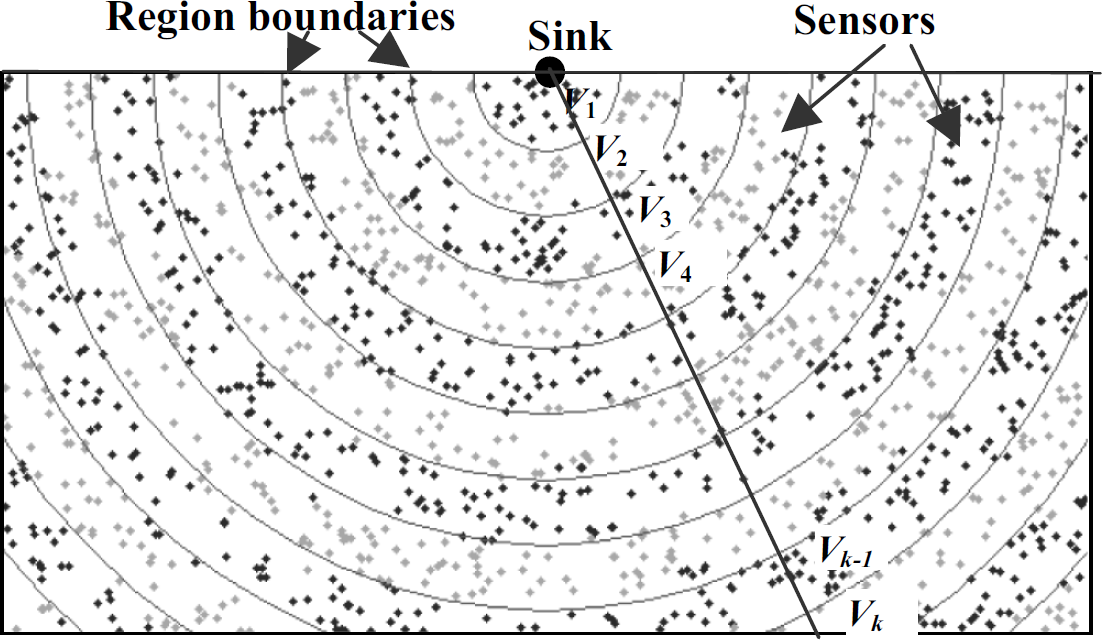
Distribution of random deployed sensors.
The existing approaches focus on minimizing the average energy cost while overlooking the energy depletion rate of sensors in Region-1. Furthermore, the existing approaches use the average total energy cost of queries to measure the performance of query processing. In fact, the average energy cost is not a proper performance metric. An approach using smaller average energy per query does not mean that it is better in terms of query capacity, and this situation is illustrated in Fig. 2. In Fig. 2, the sink has two neighbors, s1 and s2. Assume that an algorithm B1 is applied in the query zone Q1 (Fig. 2(a)) and B2 in Q2 (Fig. 2(b)). Assume that B2 consumes twice the amount of average total energy per query response of B1. For each response, B1 uses two paths to send data to the sink and B2 uses a single path through either s1 or s2. Not considering the energy available in s1 and s2, sensors in Q2 deplete their energy faster than sensors in Q1. However, to transmit one query response to the sink, B1 consumes twice the amount of energy of sensors in Region-1 compared to B2. In Fig. 2(a), s1 and s2 may exhaust their energy faster than the sensors s1 and s2 in Q2 (Fig. 2(b)). Hence, B2 can deliver more query responses than B1, even though B2 consumes more energy than B1 in total.

Energy consumption of neighbors of the sink.
Query processing works in two phases [3, 4]: query distribution and data collection. In the query distribution phase, the existing approaches use either global flooding or wedge flooding to distribute queries and construct routing trees (RT). In global flooding, queries are flooded to all sensors in the network. In wedge flooding, sensors within a wedge area (approximately bounded by two dashed lines in Fig. 3) join the flooding process. High cost is the major drawback of flooding. Even though wedge flooding consumes less amount of energy, there is no guarantee that a query will be delivered to all the sensors in the query zone. The probability of query delivery can be increased by using a large flooding angle θ (Fig. 3) at a higher cost.

Illustration of query flooding in a WSNET.
The existing approaches use flooding to build RTs rooted at the sink for all query types. Consequently, sensors in Region-1 incur a high energy-consumption cost in data collection. As shown in Fig. 3, if wedge flooding is used to construct the example RT rooted at the sink, most of the sensors in the intersected area between Region-1 and the wedge area with flooding angle θ have forwarding tasks. For the non-holistic queries, the number of forwarding sensors in Region-1 is proportional (by a factor between 0.4 and 0.8) to the number of sensors in the intersected area, as shown in the supplemental document. For holistic queries, such as Median, results of sub-aggregations at intermediate sensors can not offer the correct result at the sink [3], and, thus, all raw data need to be sent to the sink. The energy consumption of sensors in Region-1 per query response is proportional to the number of sensors in the query zone. However, in either case, if the query response can be computed by a sensor within the query zone, only a constant amount of energy of sensors in Region-1 is required to transmit the response to the sink.
The existing approaches overlook the need to reduce the RX cost. If the TX distance is large, the TX cost is much larger than the RX cost. However, for realistic sensors such as Mica Mote [4], the RX cost is close to the TX cost. Hence, the RX cost needs to be factored in.
Related Work
A number of research results have been published both in network and database domains on energy-efficient query processing for WSNETs. In the network domain, research results have been published on energy-efficient routing protocols for WSNETs, such as SPIN [15], LEACH [14], and Directed Diffusion [11]. SPIN is recognized as the earliest work on data centric routing and is proposed to address the deficiency of flooding. SPIN saves sensor energy by reducing duplicate copies of messages in the classic flooding and by using meta-data to reduce the lengths of transmitted original data. Moreover, SPIN uses negotiation to help ensure only useful information is transferred. LEACH is a scalable adaptive clustering protocol in which nodes are organized into clusters. Sensors in a cluster communicate with the cluster header (CH) and CH directly transmits the processed data to the sink. LEACH uses a random process to vote CHs to balance the energy consumption of CHs, and, the system lifetime is therefore extended. Directed Diffusion is another data centric protocol in which sinks periodically floods queries into the network. During the flooding, sensors set up gradients of data propagation. Based on the received data, sinks select and reinforce some “good” paths for further data delivery.
In the database domain, Madden et al. [3, 4] proposed TAG to reduce the energy cost of processing aggregative queries by in-network aggregation techniques. In TAG, an RT is built by using flooding or wedge flooding. TAG adaptively adjusts the sampling rate of sensors based on the query constraints and energy of sensors. Through reducing sampling rates, energy spent on sensing is reduced. Cougar [5] also addressed query processing by investigating such techniques as partial aggregation and data packet merging to reduce the packet payload. Many other works have also been proposed based on TAG to address energy-efficient query processing, such as TinA [6] and location aware routing [7]. TinA utilizes the temporal coherence among data collected from the same sensor to reduce the number of transmissions. The location aware routing technique builds RTs with the goal of reducing message size for group by queries.
The preceding techniques normally assume that homogeneous sensors are uniformly distributed, which leads to a serious energy drainage problem of sensors in Region-1. To solve this problem, two techniques have been proposed:
A power-cost metric based on both node lifetime and distance-based power metric has been used to compute the shortest weight path to slow down the rate of energy consumption in Region-1. In [18], a clustered model has been presented by equipping sensors with power-adjustable transmitters. The network is partitioned into clusters and each cluster has a cluster header (CH). Each CH aggregates data received from sensors and then directly sends the aggregated data to the sink. Other sensors send data to CHs through a multi-hop or single-hop path. By interchangeably applying single-hop and multi-hop paths, energy consumption of sensors is balanced. In [19], a non-uniform sensor distribution model has been proposed, where the sensor density is higher in the sub-area closer to the sink so that all sensors deplete their energy at the same time.
For dense and stationary sensor networks, location-based routing techniques [9, 13, 20, 21] are suitable to route sensed data from sensors to the sink due to the low cost of path discovery. In the greedy forwarding algorithms [17, 21], each node chooses a neighbor, which is closest to the destination among all its neighbors, as the forwarding node. However, these algorithms have no guarantee of message delivery if a “hole” (an area without sensors) is on the forwarding direction. To remedy this problem, the Greedy-Face-Greedy (GFG) routing [13] and Greedy Perimeter Stateless Routing (GPSR) [20] have been proposed. For dense networks, the average length of the forwarding paths established by the location-based routing are roughly identical to the average length of the shortest hop paths.
We propose a Broadcasting Based query Scheme (BBS) to address the problems discussed in Section 2.1. BBS consists of five basic steps and two optional steps. The basic steps are query distribution, local RT construction, data collection, data forwarding, and sink coordination. The optional elements are local RT combination and route redirection. All basic steps are required to accomplish a query task, and the optional steps are designed to slow down the energy depletion rate of sensors near the sink.
Network Model and Terminology
A simple network model is defined to illustrate BBS. The network area is a fixed W × H rectangular area. N homogeneous, stationary sensors are randomly placed in the network area according to Poisson distribution with density λ. Each sensor has a unique ID. A network has one stationary sink with unlimited energy. Two nodes (sensor or sink) are said to be neighbors if they are within the TX range, denoted by rs, of each other. The link between two sensors is symmetric. All nodes know their locations which are required by zone-based queries. Each query zone is a rectangular area. We assume the existence of a neighbor discovery protocol and a TDMA-like MAC protocol [22, 23, 24, 26] to solve the media contention problem.
The average degree, denoted by g, of a network is the average
number of neighbors for all nodes. For randomly distributed sensors, g =
λΠ rs2. For a given zone-based query, sensors
can be classified into three types: sensing, forwarding, and normal sensors as follows. A sensing sensor of a query is a sensor within the query zone with sensing
tasks. A special case is that if the sink falls in the query zone, the sink is treated as a sensing
sensor. A forwarding sensor routes sensed data to the sink, but it does not perform
sensing task. A normal sensor of a query is a sensor which is not of the above two types.
The type of a sensor is query-dependent. A sensing sensor of a query Q1 can be a normal sensor of another query Q2. We propose query capacity as a performance metric of BBS as follows.
Definition. Query capacity, denoted by C, is defined as the total number of complete query responses received by the sink when the lifetime of the network is over.
The network lifetime is defined as the time from the initial start of the network to the moment that a certain fraction of sensors is disconnected from the sink [16]. If the sink receives several packets related to the same query, these packets are used to build one complete query response.
Query Classification in BBS
One goal of BBS is to provide a general scheme to support most of the query types for zone-based
queries. When a query is issued into a given zone, all sensors in the zone contribute to the query
response. BBS focuses on both holistic queries and non-holistic queries. Non-holistic queries have a
common feature: sub-aggregation of sensed data is allowed, that is, both raw data and aggregated
data can be stored into a constant length packet [3]. Similar to Directed Diffusion [11], a typical query supported in BBS has the following form:

In BBS, two types of messages are used: query message and response message. Each query message has four fields: {header, ID, query specification, and option}. The header field contains control information related to the query. Each query has a unique ID. The query specification contains information about the query task. The option field carries optional information and may be empty in some cases. Each response message carries a partial or complete response with five fields: {header, ID, sequence number, option, and data}. Similar to that of a TCP/IP packet, the header field specifies the source and the destination of this message. The ID makes an association of a response with a query. The sequence number is used to distinguish responses for the same query in different time intervals. The data field stores the raw data or aggregated data.
Query Distribution in BBS
BBS can distribute queries by using existing flooding techniques without influencing the rest of the basic steps. However, to avoid the flooding cost, BBS applies an optional solution by having the sink broadcast queries by using a high power transmitter [14, 17, 18] so that all the sensors hear a query directly from the sink. Equipping the sink with a power adjustable transmitter is not a significant concern. However, to use such a sink, we need to solve two consequent problems: synchronization between the sink and sensors and construction of RTs. Since the sink broadcasts queries instead of flooding, RT construction should not depend on the path information obtained during flooding, which will be addressed in Section 3.4.
When the sink has a power adjustable transmitter, synchronization between the sink and sensors can be solved as follows. During the initialization stage, the sink broadcasts a control message to synchronize all sensors. A control message is in the form of (T, Δt) which means that after T time units, the sink will occupy the channel for Δt units. During the time interval [kT, kT + Δt], where k is a positive integer, the sink broadcasts a query message or a control message. According to the control message, sensors will periodically listen to the channel in the specified interval [kT, kT + Δt]. When the sink is silent during [kT + Δt, (k + 1)T], sensors can communicate to their neighbors. Thus, BBS establishes a virtual channel from the sink to all sensors. Hence, queries can be immediately distributed to all sensors without flooding the network. Furthermore, the sink can adjust T using the next control message to delay the incoming queries. The value of T is application specific and is determined by the network environment and workload.
Routing Tree (RT) Construction in BBS
The main feature of BBS is that BBS constructs localized RTs within query zones and the RTs are rooted at sensors within the query zones. To build RTs, each sensor only needs to know the sink location, the area of query zone, and the locations and IDs of its neighbors. Hence, BBS builds RTs independent of the query distribution techniques—sink broadcasting or flooding.
Construction Steps
RT construction is based on the idea of location-based routing [9, 13, 20, 21]. The major characteristic of localized RT construction is that no path information to the sink is required by sensors. To build RTs, sensors need to know the locations and IDs of their neighbors, the query zone, and the sink. Only sensing sensors join the RT construction process. In RT construction, sensors in a query zone are organized into one or more local RTs. These RTs are rooted at some selected sensors, called local roots, within the query zone. Sensing sensors are of two types: internal tree node (internal node) and local root. An internal node is a sensing sensor with a parent on an RT. A local root is a sensing sensor without parents on an RT. The construction steps are as follows and the formal description is given in Fig. 4.

Constructing a routing tree.
Step 1. Computation of the root reference point and determination of sensor priorities Initially, all sensing sensors compute the coordinate of a unique geographical point within the query zone, called root reference point. The selection of the root reference point is query type dependent and is discussed later. Each sensing sensor si is assigned to a unique priority level defined as Pi = P(di, IDi), where di is the Euclidian distance from si to the root reference point and IDi the identifier of si. For any two sensing sensors si and sk, P(di, IDi) > P(dk, IDk) iff the condition (di > dk) ‖ ((di = dk) && (IDi > IDk)) is true, where && and ‖ are logical AND and OR operators, respectively. The meaning of a higher priority is that the sensor has a shorter distance to the root reference point. In the case of two identical distances, the sensor with a larger ID has higher priority. Due to the uniqueness of IDs, each sensor gets a unique priority.
Step 2. Local root selection Sensing sensors determine if they are local roots as follows. For a sensing sensor si, let ψi denote the set of neighbor sensing sensors of si. If si has the highest priority (discussed in Step 1) over all sensors in ψi, then si becomes a local root. If si is not a local root, si is an internal node. There is one exception, however: for non-holistic queries, if the sink is not located in the query zone, all sensing sensors in Region-1 are local roots. This special case avoids transmissions between two one-hop neighbors of the sink, and reduces the energy consumption of nodes in Region-1.
Step 3. Parent node selection Each internal node must select one sensing sensor as its parent node. For an internal node si, let di and ψi have the same meanings as defined in Steps 1 and 2. si selects a sensing sensor sk, where sk (ψi and sk has the highest priority over all sensors in ψi, as its parent. If si has its parent node sk, si is called a child node of sk. Obviously, local roots do not have parents. Moreover, we say that there is a child-parent relationship between si and sk.
If we treat sensing sensors as nodes and the child-parent relationships as edges, a directed RT
graph is formed with the following properties, which are proved in the supplemental document. RT Graph P1. The graph contains all sensing sensors, but no normal sensors. RT Graph P2. The graph has no cycle, but contains one or more trees
(local RTs). RT Graph P3. Each local RT is rooted at exactly one local root and each local
root is located on exactly one local RT.
Figure 5 shows an example RT construction based on the preceding algorithm. In Fig. 5, sensors s1 and s2 are selected as local roots since they have the highest priorities over their neighbors. The other sensors choose their parents according to the priorities of neighbor sensors.

RT construction and root reference point for a given query.
Different query types have different requirements for the structure of constructed local RTs. The root reference point has an important impact on the structure of local RTs, and hence different root reference points are used for different query types. In BBS, for all query types, if the query zone covers the sink, the root reference point is the location of the sink, and the sink becomes a local root. For other cases, the root reference point is query dependent.
For non-holistic queries, the root reference point is the intersected point between one edge of the query zone and the line segment connecting the sink and the center of the zone (R1 in Fig. 5). This implies that in most of the cases sensors close to the sink have a higher probability to be selected as local roots, which reduces the forwarding cost and delay from local roots to the sink.
For holistic queries such as Median, the root reference point is the center point of the intersected area of the query zone and the network area (R2 in Fig. 5). This selection is determined by the special feature of Median: any aggregations on the forwarding path will affect the final result. The existing approaches can not efficiently process Median like zone-based queries since all sensor readings should be sent to the sink without data aggregation. This process consumes a large amount of energy of sensors in Region-1. Even though no sub-aggregation is allowed, a local root can collect all sensor readings within the query zone, compute the value of Median, and send the value to the sink in a single packet. In this way, the energy depletion rate is slowed down for sensors in Region-1. However, this solution works only if one local RT exists in a query zone. If two or more local roots exist in a zone, they do not have information about each other. Each of them will transmit the computed Median to the sink. But the sink can not extract the correct value from the received multiple Medians. This problem for the multiple computed Medians (or other holistic queries) is called sub-aggregation problem. The center of a query zone is selected as the root reference point due to two reasons. First, if the root reference point is located on one boundary of the query zone, sensing sensors close to this boundary have small areas in which their parents can be located. Hence, these sensors have higher probability to be a local root. Second, the longer the distance from a sensor to the root reference point, the higher the probability the sensor can not find a parent by using location-based techniques, which results in multiple RTs. The average distance from all the sensing sensors to the root reference point is minimized if the center point of the zone is used. To minimize the probability to construct multiple RTs, the zone center is used as the reference point.
Data Collection within Local RTs
After local RTs are constructed, each parent is responsible for collecting sensed data from all its children, and aggregates the data if possible. This process can be accomplished by a technique similar to the one proposed in the TAG approach [3] with some modifications as follows.
Sensors sense the environment periodically according to the time intervals specified in queries. All sensed data in the same interval, called a round, generate a complete query response. In the first round, each parent waits until all its possible children transmit their data. By using the information of source and destination nodes in the received packets, the parent knows its children. The parent processes the received data and its reading, and sends the data to its parent. In the later rounds, each parent listens to the channels of its children periodically. In this case, a TDMA-like MAC layer support [22, 23, 24, 26] is desired, where sensors can decide if they go to sleep mode to save energy. There is one exception for holistic queries: sensors, except local roots, must transmit raw data to their parents. In this case too, energy can be saved by a parent combining several packets into one to remove the original multiple header fields.
The workload of local roots may be perceived to be very high, leading to their fast depletion of energy. However, localized RTs still prolong the lifetime of a sensor network compared with the existing approaches due to the following reason. Without using local RTs, the bottleneck of the query capacity is the total energy of the sensors in Region-1. In real applications, query zones are distributed in the network area. With using local RTs, different query zones select different sensors as their local roots, resulting in that the total number of local roots for all queries is much larger than the neighbor sensors of the sink. Hence, the bottleneck related to the neighbor sensors in Region-1 is more severe than the bottleneck created by the high workload of all local roots and the high workload of all local roots has no significant impact on the query capacity.
Data Forwarding in BBS
After the local roots collect all sensed data from their children, those compute the query response and forward it to the sink. This involves two steps: find a forwarding path to the sink and aggregate data if possible.
Forwarding Path Establishment
Since all sensors are likely to be selected as local roots, they need to maintain forwarding paths to the sink. If BBS uses flooding to disseminate queries, the forwarding paths are established during flooding and there is no additional cost for discovering a routing path. On the other hand, for BBS to use a power adjustable sink to broadcast queries to all the sensors, each local root needs to find a forwarding path to the sink. Since sensor networks consist of densely deployed stationary sensors, location-based routing algorithms are good candidates for data forwarding [9, 13, 20, 21]. In location-based routing, each local root knows the locations of its neighbors and the sink. During the forwarding process, each local root chooses a neighbor sensor, which is closest to the sink among all its neighbors, as the next forwarding node. This forwarding strategy is known as the “greedy” principle [9]. The major advantage of this technique is that no flooding is required to build routing paths. Its disadvantage is that delivery of responses is not guaranteed. For sparse networks, GFG [13] or GPSR [20] can be used to guarantee message delivery. For dense sensor networks, the preceding algorithms have a very low cost of routing path discovery and maintenance, and, therefore, the cost can be ignored.
Data Aggregation during Forwarding
In the data forwarding process, query responses can be forwarded to the sink from local roots by using the algorithms in references [9, 13, 20]. The sensors on forwarding paths are called forwarding sensors. Forwarding sensors process received data in different ways for different query types. For holistic queries, forwarding sensors simply forward received messages to the sink. For non-holistic queries, forwarding sensors perform data aggregation as follows.
For data aggregation, forwarding sensors use a sub-field, called REP#, in the option field of the query response message. The option field also contains the ID of the local root which will be used in local RT combination (Section 4.1). When a local root issues a query response message, it sets REP# to be one. During the first round of forwarding, each forwarding sensor s records query IDs and sequence numbers of the queries from received response messages. Then s forwards the data to the next node immediately. When s receives more than one response related to the same query ID and sequence number, it sums up the values (denoted by Ns) of the REP# fields from all responses related to the same query and sequence number. Thus, Ns equals to the number of local roots that forward their query responses through s. In each upcoming round, s waits for a time period to collect partial query responses and sum up the values of REP# as it is done in the first round. In the cases that either the summation equals to Ns or time-out occurs, s aggregates the received responses into one packet, sets the REP# to the value of summation, and sends the packet to the next node. This method supports data aggregation at forwarding sensors and guarantees that one copy of each sensor reading contributes to the final query response.
Sink Coordination in BBS
Even though all sensing sensors are internally connected in a query zone, multiple local roots may exist when a local RT is constructed. For holistic queries, multiple local roots cause the sub-aggregation problem (Section 3.4.2). For non-holistic queries, the multiple local roots choose their forwarding paths independently, which may result in two or more sensors in Region-1 being on the forwarding paths. To solve the sub-aggregation problem and to reduce the number of sensors in Region-1 involved in data forwarding, the sink can make an attempt to combine all local RTs into one RT by using localized flooding within the query zone. This process is called local RT combination and will be discussed in detail in Section 4.1.
For holistic queries, the sub-aggregation problem can be detected after the sink receives two or
more computed Medians with the same query ID and sequence number. The sink can solve this problem in
two alternative ways as follows: Solution 1: The sink informs all local roots to send raw data to the sink. The sink can either
use its high power transmitter to broadcast a control message or send the control message via
multi-hop paths established during data forwarding to all local roots. After receiving such a
control message, local roots start sending raw data. Solution 2: The sink performs local RT combination explained in Section 4.1. If all local RTs are successfully combined
into one RT, the sub-aggregation problem is solved. If the sink still receives multiple Medians, it
will use the first solution.
Optional Elements of BBS
The optional elements of BBS are local RT combination and route redirection, which aim to reduce energy consumption of sensors in Region-1.
Local RT Combination (LRC)
RT construction may generate multiple local RTs. Local RT combination is a
process whereby the sink makes an attempt to combine all local RTs into one RT by using localized
flooding to produce the following benefits: For non-holistic queries, multiple RTs may lead to more sensors in Region-1 with forwarding
tasks. Thus, a small number of RTs implies less energy consumption of sensors in Region-1. For holistic queries, LRC may solve the sub-aggregation problem (Section 3.4.2) and significantly increase the query
capacity of a network.
When the sink detects the existence of multiple local roots for a query, it sends an LRC initialization packet to all local roots via multi-hop paths or via the shared channel. This initialization packet contains the ID of the nearest local root to the root reference point. The ID of the nearest local root can be obtained during the forwarding process (Section 3.6.2). When the nearest local root receives the initialization packet, it starts LRC by flooding an LRC packet within the query zone. The parent selection of each sensing sensor is described in Fig. 6.

Parent selection of a sensor in local RT combination.
For each sensing sensor s, when s receives the first LRC packet, s sets its parent to the sensing sensor which sends the packet and s broadcasts the LRC packet to its neighbors. Duplicate LRC packets are discarded. When local roots receive an LRC packet, they become internal nodes. Sensing sensors that do not receive the LRC packet retain their original child-parent relationships established in local RT construction. The localized flooding is terminated as follows: each sensor estimates the maximum height of local RTs based on the size of the query zone, and computes a time interval when flooding can be completed.
LRC is optional and is determined by the sink. For holistic queries, if the LRC process fails to construct one local RT, each sensing sensor transmits its raw data to the sink. Similar to an RT graph built in RT construction, the child-parent relationships, among sensing sensors established by applying LRC, form a new graph, called RT-LRC graph. Since LRC uses localized flooding, it has an additional cost which is analyzed in Section 6.3.1. While satisfying the three properties of RT graphs, RT-LRC graphs satisfy a fourth property stated below.
RT-LRC Graph P4. If the topology graph within the query zone is connected, all sensing sensors belong to one RT. (The proof is given in the supplemental document).
Route redirection (RR) aims to reduce energy consumption of RXs of sensors in Region-1 and is applied only for non-holistic queries. From the network shown in Fig. 7(a), when a query zone contains three sensors s1, s2, and s3 in Region-1, we can not reduce the total number of TXs of s1, s2, and s3 since they must transmit their sensed data to the sink. However, we can reduce the number of RXs of s1, s2, and s3 by carefully redirecting routes among two-hop sensors of the sink. A k-hop sensorof the sink is a sensor whose hop distance to the sink is k. A sibling of a sensor s is a neighbor sensor of s with the same hop distance to the sink as s. In Fig. 7(b), two-hop sensing sensors of the sink redirect their sensed data to s4, and then s4 transmits the aggregated data to s2. In Fig. 7(a), the total number of RXs of the sensors in Region-1 is 5. With route redirection in Fig. 7(b), the number of RXs is reduced to 1.
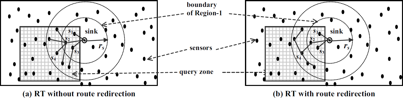
Illustration of basic idea of route redirection.
If the energy cost of RX is significantly less than the energy cost of TX, RR can not save a
significant amount of energy of sensors in Region-1. However, in real applications [4, 8, 12], the RX cost is very close to the TX cost, and, in this situation, RR leads to
significant energy saving as shown in Fig.
7. RR is applied only if the following three RR conditions are satisfied:
the query is non-holistic; the RX cost is considerably large; the query zone contains one-hop sensors of the sink. RR is performed during the local RT
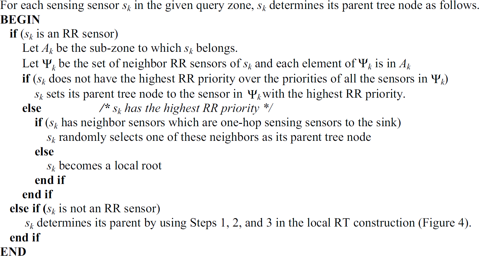
construction process as follows.
All sensing sensors except two-hop sensors of the sink determine their parent tree nodes by using the local RT construction process (Section 3.4). The RR process is only performed by two-hop sensing sensors of the sink, called RR sensors. Similar to root reference points used in RT construction, RR sensors use a redirection reference point to select their parents. For each RR sensor sR, it belongs to a unique sub-zone Qs, which has a unique redirection reference point—the exact description is given later. Similar to using the root reference point to compute sensor priorities in RT construction, sR computes its RR priority by using its redirection reference point. The meaning of RR priority is this: the shorter the distance from an RR sensor to its redirection reference point, the higher the priority of the sensor. sR also computes the RR priorities of its sibling RR sensors which are in the sub-area Qs. If sR does not have the highest priority among these siblings, sR sets its parent to the sibling with the highest priority among all sibling RR sensors. If sR has the highest priority among all siblings, sR checks the set (denoted by ψR) of its neighbor sensing sensors which are one-hop to the sink. If ψR is not empty, sR sets its parent to the sensor in ψR nearest to the root reference point— not redirection reference point. If ψR is empty, sR becomes a local root.
To accomplish RR, each RR sensor must determine its sub-zone and redirection reference point,
which avoids cycles in the constructed RTs and reduces the height of RTs. Let
AR denote Region-1 and AQ the query zone.
Since RR is performed only if the query zone contains sensors in Region-1,
AR ∩ AQ > 0, where ∩
denote the intersection of two areas. A sub-zone Ak is defined as a
sub-area of AQ satisfying four conditions: Ak is enclosed by two or more line segments and one arc, each boundary line segment of Ak is a portion of the boundary of
AQ, the boundary arc of Ak is a portion of the boundary of
AR, and any two sub-zones are disjoint.
Figure 8 illustrates the partitions of sub-zones, which depend on the intersected points of the boundaries of A R and AQ. In Fig. 8(a), the boundaries of AR and AQ intersect at points B and C, and there exists one sub-zone—the shaded area—enclosed by line segments BO, OP, PQ, QC and the arc CDB (shortened as the list of endpoints BOPQCDB). In Fig. 8(b), three intersected points D, E and H forms two sub-zones DOPHFD and ERQHGE (two shaded areas). Since each sub-zone has exactly one arc as a part of its boundary, the midpoint of the arc is the redirection reference point of the sub-zone. In Figure 8(a), D is selected as redirection reference point.

Basic cases of route redirection.
One exception for the preceding description is shown in Fig. 8(c) where the query zone covers Region-1 without intersected points on their boundaries. In this case, the query zone is separated into two sub-zones by the line connecting the sink and the center (point K) of the query zone. This line intersects Region-1 at points M and N. The midpoint I of the arc MIN is selected as the redirection reference point for the sub-zone above the line MN. The purpose of this partition is to avoid long paths. A formal description of RR is given in Fig. 9.
Distributed algorithm of route redirection.
Similar to RT graphs in Section 3.4, the child-parent relationships among sensing sensors established by applying RR form a new graph, called RT-RR graph. RT-RR graphs retain all the properties of RT graphs. The proofs are given in the supplemental document.
Since one-hop sensors are more important than other sensors, energy conservation of one-hop sensors is the primary task of RR. Even though RR can be applied to three-hop or higher hop sensors, it increases the height of RTs, leading to longer delay. To balance the gain and the cost, only two-hop neighbors are considered. The cost of performing RR is given in Section 6.3.1.
BBS Operations, Network Model and Performance Metrics
Figure 10 demonstrates the operation sequence of BBS. The paths marked by dashed arrows in the figure denote optional elements. In BBS, queries can be distributed by flooding or broadcasting from the power-adjustable sink. Then RTs are constructed in local RT construction phase. For non-holistic queries, route redirection is also performed in this phase. After the local roots receive all data from their children in the data collection phase, the local roots process and forward the data to the sink in the same data collection phase. When the sink receives the data, it determines whether the local RT combination process is to be performed. To distinguish BBS with different elements, we use BBS-Null (or simply BBS), BBS-RR (or simply RR), BBS-LRC (or simply LRC) to denote BBS without any optional elements, BBS with route redirection, and BBS with local RT combination, respectively.

Operational sequence of BBS.
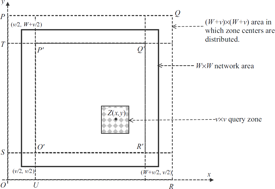
Performance analysis of BBS is based on the network model in Section 3.1 with some modifications. To simplify the analysis, we constrain the network area to a W × W square area, and the sink is located at the center of the network area. Each query zone is a v × v square area. We assume that all sensors have equal probability to be queried. This assumption requires that centers of query zones are randomly distributed within a (W + v) × (W + v) square area (Fig. 11). This model is called a Single Stationary sink Center placement model (SSC model) and its related network is an SSC network [3, 10, 14, 19]. Each SSC network can be specified by seven parameters (W, v, g, Ps, etx, erx, rs), where g is the average degree of sensors, Ps is the initial energy of sensors, etx is the TX cost, erx is the RX cost, and rs is the TX radius of all sensors. Hence, the total number of sensors (denoted by N) in the network is N = (g + 1)W2/(rs2).

Distributed area of zone centers.
Energy consumption can be divided into two parts: the cost for query distribution and RT construction, and the cost of data collection and data forwarding. The second cost reflects the effectiveness of RT
construction.
In this section, we analyze the second cost by using query capacity C as the
performance metric. The first cost will be analyzed in Section 6.3. Hence, we assume the existence of local RTs
and ignore their construction costs. Due to space limitation, we only estimate C
for BBS-Null supporting non-holistic query in a given SSC network with
Due to the fast energy depletion rate of sensors in Region-1, C approximately
equals to the number of query responses collected by the time all sensors in Region-1 exhaust their
energy. Since the sink has g neighbors and the RX cost is negligible, the sink can
receive at most gPs/etx number of TXs. From
the assumption that one response is collected for each query, there are C queries
generated randomly. These queries can be classified into two types: query zones have at least one sensor in Region-1; query zones do not have sensors in Region-1. Obviously, these two types of queries are
disjointed, and, therefore, the summation of total numbers of TXs from sensors in Region-1 involved
in these two types of queries should equal
Then we can estimate the numbers of TXs separately in these two types of queries. Due to space
limitation, we give the final result of C as follows, and the detailed derivation
is shown in the supplemental document.

where h is the positive solution of the equation
In this section, we evaluate the predicted query capacity in (1) and compare the performance of
BBS against the TAG approach [3] since
TAG is the most well-known general query processing scheme. We compare BBS and TAG in two parts:
efficiency of RTs in data collection and forwarding; energy consumption in query distribution and RT construction. The first part is done by using
simulation studies and the second part is done analytically.
Simulation is done by using a routing-level simulator, operating on randomly generated SSC
networks. For each sample SSC network (W, v, g, Ps, etx,
erx, rs), we fix Ps = 500,
W = 100 and vary other parameters. We set the TX and RX costs in an abstract
sense to reflect two scenarios: the TX cost is dominating and the RX cost is negligible, and the two costs are comparable.
In the former case, etx = 10, erx = 0. In the latter case, etx = 5, erx = 5 (derived from the real data of Mote [4]). Each simulation uses a set of randomly generated v × v query zones and RTs are built once for each query. When a sensor depletes its energy, it is removed from the network. If more than 10% of the sensors are disconnected from the sink, we terminate this simulation and record its query capacity. All reported results are computed by taking the average of 20 sample runs.
Equation (1) in Section 5.2 computes the query capacity of a given SSC network (W, v, g, Ps, etx, erx, rs) with erx = 0 by applying BBS-Null. Figures 12 and 13 illustrate the predicted results by (1) (denoted by BBS-P) and the simulated results (denoted by BBS). From these figures, we conclude that the predicted results closely match the simulated results.

Query capacity (g = 10, etx = 10, erx = 0, rs = 10).

Query capacity (g = 20, etx = 10, erx = 0, rs = 5).
In this sub-section, we compare the efficiency of RTs built by TAG and BBS for two types of queries: non-holistic query (Max) and holistic query (Median). Query capacity is used as the performance metric in this comparison. We ignore the cost of query distribution and RT construction, which will be discussed in Section 6.3.
Simulation Results for Non-holistic Queries
Figures 14 through 17 give the simulation results for non-holistic queries. We vary four parameters g, etx, erx, and rs in our simulations. If erx = 0, BBS does not use RR. Therefore, Figs. 14 and 16 do not have the results of BBS-RR. In Figs. 15 and 17, we do not show the result of BBS-LRC because its performance is slightly higher than BBS-Null. According to the simulation results, BBS-Null, BBS-RR, and BBS-LRC outperform TAG. The improvement in query capacity is in the range of 10% to 100%. In addition, we have the following observations.

Query capacity (g = 5, etx = 5, erx = 0, rs = 10).

Query capacity (g = 20, etx = 5, erx = 5, rs = 10).

Query capacity (g = 20, etx = 10, erx = 0, rs = 10).
First, according to the results in Figs. 15 and 17, if the RX cost is not negligible, BBS-RR improves the performance compared with BBS-Null. The larger and denser the network is, the higher the performance gain. However, compared with BBS-Null, the performance improvement of BBS-RR is not significant. This is because we assume a uniformly distributed query zone in the network area. RR is performed only if the query zone contains sensors in Region-1. The probability of query zones satisfying this condition is small (Section 5 in the supplemental document). Hence, the performance gain is not obvious. For the experiments in which all query zones satisfy this condition, the performance gain can be up to 50%, as shown in the example in Fig. 7. Second, BBS-LRC slightly outperforms BBS-Null. This is due to two reasons. One is that the number of local roots tends to 1 for dense networks and there is no need to perform LRC. The other reason is that there is a possibility that multiple paths from local roots may join together at a node near the sink. Third, the density and size of a network affect query capacity. The query capacity improvement in Fig. 17 is much higher that the one in Fig. 14, suggesting that BBS works better for large and dense networks. Finally, BBS has a higher performance gain for small and medium size query zones. When the query zone size is close to the size of the network area, the performance gain of BBS is not obvious.

Query capacity (g = 20, etx = 5, erx = 5, rs = 5).
Tables 1–4 show the query capacities for Median by using TAG, BBS-Null (BBS in the tables) and BBS-LRC (LRC in the tables). In TAG, all sensor readings are forwarded to the sink without aggregation. In BBS-Null, if there are two or more local RTs, all sensor readings are sent to the sink as TAG does. In BBS-LRC, if two or more local RTs exist, LRC is performed. Since we focus on the effectiveness of the constructed RTs, the cost of LRC is ignored here—which is discussed in Section 6.3. The network configurations are shown in the table titles. In all the tables, data in the first row denotes the width of square query zones.
Capacity of network (g = 10, etx = 5,
erx = 0, rs = 10)

Capacity of network (g = 10, etx = 5, erx = 0, rs = 10)
Capacity of network (g = 20, etx = 5, erx = 0, rs = 10)

Capacity of network (g = 10, etx = 1, erx = 0, rs = 5)

Capacity of network (g = 20, etx = 1, erx = 0, rs = 5)
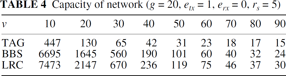
According to the results in these tables, we conclude that BBS-Null and BBS-LRC significantly outperform TAG. Furthermore, the larger and denser a network is, the larger is the performance gain obtained by applying BBS-Null and BBS-LRC. The improvement of query capacity can be up to an order of magnitude for large and dense networks. By comparing the results of BBS-Null and BBS-LRC, we find that BBS-LRC is significantly superior to BBS-Null in sparse networks (g = 10) and moderately better than BBS-Null in dense networks (g = 20). In dense networks, the local RT construction process is likely to build one local RT in the query zone, and hence it is unnecessary to perform LRC in most cases.
In this section, we compare the energy consumption of query distribution and RT construction in BBS against the one used in TAG (global flooding or wedge flooding). Obviously, if BBS employs the same flooding technique used in TAG, BBS and TAG have the same energy consumption. However, in BBS, if the sink is equipped with a power adjustable transmitter, BBS consumes much less energy than TAG, which is verified in this sub-section.
The cost is measured by using two metrics. The first metric, denoted by Ed, is the total energy consumed by all sensors in query distribution and RT construction. The second metric, denoted by Ec, is the energy consumption of sensors in Region-1, including the total energy consumption of all TXs and RXs of sensors in Region-1. Since the total energy of sensors in Region-1 is the bottleneck of the query capacity of an SSC network, Ec is more useful than Ed. For simplicity, we assume that the following analysis is based on the query zones without sensors in Region-1.
Cost of BBS with Power Adjustable Sink
Several operations are involved to distribute queries and construct local RTs. These are query
distribution, local RT construction, RR, and LRC, and let their individual costs be
ed, ec, er, and el,
respectively. The reader may note that the costs of RR and LRC are independent of whether or not a
power adjustable sink is used. For a given SSC network (W, v, g, Ps,
etx, erx, rs), since all
sensors receive a query from the shared channel, we have ed =
erxN. The cost of local RT construction and RR consists of two parts: the cost
of computations of sensor priorities and the cost of neighbor discovery. The computation cost can be
ignored compared with the TX and RX cost [17, 4]. However, the neighbor
discovery cost depends on the applied network environments. In relatively stable environments where
the sensor failure rate is very low, the neighbor discovery protocol is executed infrequently
compared with the frequency of queries. In this situation, this cost can be ignored and
ec + er ≈ 0. In an unstable environment, the
neighbor discovery process is executed for each query. In this process,
Nv2/W2 sensors are located in the query
zone, each of them broadcasts once, and each hears messages from g neighbors on an
average. Hence, the neighbor discovery cost per query is ec+
er ≈ (etx + gerx)
Nv2/W2. In LRC, one local root needs to
initiate a flooding within the query zone. The average number of sensors in a query zone is
Nv2/W2. During flooding, each sensing sensor
has exactly one TX and approximately g number of RXs from its neighbors, which
gives us el ≈ (etx +
gerx) Nv2/W2. Thus, for
BBS without LRC, we have the following results: for stable environment: for unstable environment:


For BBS with LRC, for stable environment: for unstable environment:


The estimation of Ec is straightforward: the only cost is from
receptions of the query message of sensors in Region-1. Therefore, we have 
Since each sensor broadcasts once, the number of TXs is N. Since each sensor
will receive flooding packets from all its neighbors, the total number of RXs in a SSC network is
approximately equal to gN. Thus, 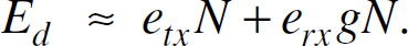
To estimate Ec, we recall that there are about g
number of sensors in Region-1. Each of them receives about g number of flooding
packets. Thus, 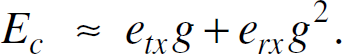
We use Fig. 3 as a part of SSC network
for the analysis. Let Aw denote the area of the wedge region and
θ the angle of the wedge area in Figure
3. The total number of sensors in the wedge area can be estimated as
NAw/W2, and the total number of RXs
approximately equals to gNAw/W2. Thus we
have 
The number of sensors in Region-1 involved in wedge flooding is determined by θ, and this
is approximately equal to gθ/(2π). Hence, the number of TXs is
g θ/(2π). It is not easy to estimate the number of RXs involved of
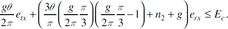
sensors in Region-1. Instead, we provide a lower bound and an upper bound for θ ≤
π/3. First, all sensors in Region-1 receive the query message from the sink, and the number
of these RXs is g. If n2 denotes the total number of
two-hop sensors of the sink within Aw, then the maximum number of RXs is
bounded by gθ/(2π)(gθ/(2π) − 1
+ n2) + g. When θ ≤
π/3, all sensors in the first critical region can hear each other and there are at least
n2 number of RXs from two-hop neighbors to the sensors in Region-1, the
lower bound of the number of RXs is
gθ/(2π)(gθ/(2π) − 1)
+ n2 + g. Hence we have: 
When θ > π/3, the upper bound is unchanged and the lower bound becomes
These two bounds are loose bounds. In fact, Ec is much larger than the lower bound since we only count one RX of sensors in the first critical region for each TX from a two-hop neighbor.
According to the preceding analysis, with a power adjustable sink, BBS can have significant advantage over flooding in terms of the total energy consumption and the energy consumption of sensors in Region-1 in query distribution and RT construction. Another advantage of BBS is that the delivery of queries is guaranteed with a constant delay. Wedge flooding does not have this guarantee if θ is small. If a large θ is used to make query delivery reliable, the cost increases accordingly. Global flooding guarantees query delivery, but it consumes a significant amount of energy. The cost in BBS-LRC is higher than BBS-Null. However, as the results in Section 6.2.2, the performance gain due to using LRC is significant in sparse networks compared to BBS-Null.
Concluding Remarks
Energy conservation is a major concern in query processing in WSNETs. For WSNETs with uniformly
distributed homogeneous sensors, current techniques for query processing have four drawbacks: overlooking the fact that sensors near the sink exhaust their energy sooner; building uniform RTs rooted at the sink for all queries; disregarding the need to reduce the data reception cost; and ignoring the flooding cost of query dissemination.
In this paper, we propose a novel energy-efficient query scheme BBS to address the above drawbacks. BBS models a complete query operation into five basic steps: query distribution, RT construction, data collection, data forwarding, and sink coordination. In query distribution, the sink may use a high power transmitter to broadcast queries to all sensors to eliminate the flooding cost. In RT construction, BBS builds localized RTs rooted at sensors within a query zone. In data collection, sensors collect the sensed data, aggregate the data if applicable, and send the data to their parents. Then, each local root uses the existing (location-based) routing algorithms to transmit the query response to the sink. In sink coordination, the sink analyzes the efficiency of the current local RTs based on the responses, and takes actions (optional elements) if necessary. Furthermore, two optional operations—route redirection and local RT combination —have been designed in BBS to slow down the energy depletion rate of sensors near the sink.
By executing the basic and optional steps, BBS effectively slows down the energy depletion rate for the sensors in Region-1 and reduces flooding cost. Compared with TAG, the experiments show that BBS increases 10%-100% of the query capacity for non-holistic queries. For holistic queries, an order of magnitude increase of the query capacity is achieved by BBS.
Supplemental Document
This document provides the detailed proofs of all the properties and some results used in the
main paper “
The statement in Section 2.1 (B) for wedge flooding is: “For the aggregative queries, the number of sensors in Region-1 with forwarding tasks is proportional (by a constant factor between 0.4 and 0.8) to the number of sensors in the intersected area.” We evaluate this statement by using simulation studies. The simulated network environment follows the configurations of the SSC network model discussed in Section 5.1 in the main paper. The technique of wedge flooding is as follows. In the wedge flooding, each node a waits a random interval before re-broadcasting and each node selects as its parent the first neighbor that it hears with the minimum hop count. Only sensors in the wedge area join the flooding process. Let θ denote the angle of the wedge area, g denote the average degree, N1 is the total number of sensors in the intersected area of the wedge area and Region-1, and N2 the total number of sensors with forwarding tasks (in the intersected area of the wedge area and Region-1). We vary the values of g (from 10 to 30) and θ (from π/6 to π) and compute the ratio between N2 and N1 which indicates the percentage of sensors in Region-1 with forwarding tasks. All results are computed by taking an average of results of 100 sample runs. The results are shown in Table 1, which concludes the statement.
Ratio between N2 and N1 (percentage of
sensors with forwarding tasks)
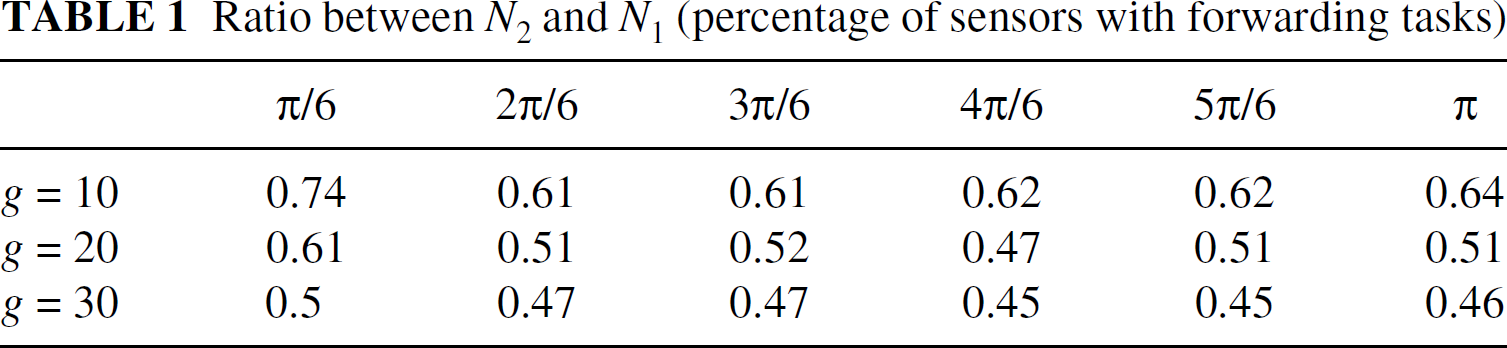
Ratio between N2 and N1 (percentage of sensors with forwarding tasks)
RT Graph P1
The graph contains all sensing sensors, but no normal sensors.
Proof. According to the description of the local RT construction process, only sensing sensors participate in this process, so the graph contains no normal sensors. Similarly, based on the three RT construction steps shown in Section 3.4.1, for each sensing sensor, it is either an internal tree node or a local root. Hence, the graph contains all sensing sensors.
RT Graph P2
The graph has no cycle and only contains one or more local trees (local RTs).
Proof. Assume that there exists a cycle in an RT graph denoted by s1, s2, … sk, s1, where s1 is a child of s2, s2 is a child of s3, …, and sk is a child of s1. Let di denote the distance from the sensor si to the root reference point. According to the construction steps 2 and 3 and the definition of sensor priorities, the distance from a given parent sensor to the root reference point must be less than or equal to the distances from its children to the root reference point. According to the cycle above, we have d1 ≥ d2 ≥ … ≥ dk ≥ d1. Thus, the only solution is d1 = d2 = … = dk = d1. From the construction steps 2 and 3, if there exists tie in terms of distances, sensor IDs are used to solve the tie. Let IDi denote the ID of the sensor si. Due to the uniqueness of each ID, we have ID1 > ID2 > … > IDk > ID1, which leads to a contradiction: ID1 > ID1. Hence, the graph contains no cycle.
Since the graph contains no cycle and each sensing sensor has null or exactly one parent, obviously the graph consists of one or more trees.
RT Graph P3
Each local RT is rooted at exactly one local root and each local root is located at exactly one local RT.
Proof. First we prove the statement that each local RT is rooted at exactly one local root. Assume that a local RT is rooted at two local roots r1 and r2. Then there exists at least one sensor which has two parents. This result contradicts the parent tree node selection rule, in which each tree node has null or exactly one parent (step 3 in Section 3.4.1). Hence, each local RT is rooted at exactly one local root.
Next, we prove the statement that each local root is located at exactly one local RT. Assume that a local root r is located at two local RTs T1 and T2. Since each local RT is rooted as exactly one local root, either T1 or T2 is rooted at a local root, which is not r. Without loss of generality, we assume that T1 is rooted at a local root r′, where r′ ≠ r. Then there should exist at least one sensing sensor s, which is a descendant of both r and r′. In this case, one of ancestors of s must have two parents, which contradicts the parent tree node selection rule. Hence, the statement is true.
Proofs of Properties in Section 4.1
RT-LRC Graph P1
The graph contains all sensing sensors, but no normal sensors.
Proof. Local RT combination (LRC) is performed after the local RT construction process. According to the descriptions of the local RT construction process and LRC, only sensing sensors participate in this process, so the graph contains no normal sensors.
Assume a local root r is selected to perform LRC and initiate the flooding within the query zone. Then all sensing sensors connected to r at the topology map of the query zone belong to the local RT (built by flooding) rooted at r. All disconnected components from r in the topology map of the query zone retain the original child-parent relationship established in the local RT construction process. According to the RT Graph P1, the sensors in the disconnected components also belong to the graph. Hence, the graph contains all sensing sensors.
RT-LRC Graph P2
The graph has no cycle and only contains one or more local trees (local RTs).
Proof. Assume a local root r is selected to perform LRC and initiate flooding within the query zone. To prove the statement that the graph has no cycle, there are two cases: (1) all sensing sensors are connected to r via paths within the topology map of the query zone; (2) not all sensing sensors are connected to r via paths within the topology map of the query zone. For the first case, since the nature of flooding, the entire graph is a local RT rooted at r without cycle. For the second case, the component, to which r belongs, has no cycle. Since all disconnected components to r retain the original tree structure established in the local RT construction process, according to RT Graph P2, they contain no cycle either. Hence, a RT-LRC graph contains no cycle. Since the graph contains no cycle and each sensing sensor has null or exactly one parent, obviously the graph consists of one or more trees.
RT-LRC Graph P3
Each local RT is rooted at exactly one local root and each local root is located at exactly one local RT.
Proof. Assume a local root r is selected to perform LRC and
initiate flooding within the query zone. We consider two cases: all sensing sensors are connected to r via paths within the topology map of the
query zone; not all sensing sensors are connected to r via paths within the topology map of
the query zone. Then we can easily show that the property holds in both cases by using the same
method used in the proof of RT Graph P3.
RT-LRC Graph P4
If the topology graph within the query zone is connected, all sensing sensors belong to one RT.
Proof. The result is obvious since the nature of flooding in the local RT combination process.
Proofs of Properties in Section 4.2
RT-RR Graph P1
The graph contains all sensing sensors, but no normal sensors.
Proof. The proof is similar as the proof given for RT Graph P1.
RT-RR Graph P2
The graph has no cycle and only contains one or more local trees (local RTs).
Proof. First we prove the statement that the graph has no cycle. The route redirection process is executed parallel with the local RT construction and only two-hop sensing sensors join this process. The established RTs by all sensing sensors, except two-hop sensing sensors, retain the properties of local RT construction. Obviously, it is impossible that there exists a connection between a one-hop sensing sensor and a three-hop sensing sensor. Hence, there is no cycle for all sensing sensors which hop distances to the sink are greater than two. Meanwhile, route redirection is performed by aggregative queries only, in which all one-hop sensing sensors automatically become local roots, so there is no one-hop sensing sensors whose parents are two-hop sensing sensors. Similarly, based on route redirection, there is no two-hop sensing sensor whose parent is a three-hop sensing sensor. In this case, if the RT-RR graph contains a cycle, this cycle must exist within two-hop sensing sensors. According to the description of route redirection, each two-hop sensing sensor is located in exactly one sub-zone and each sub-zone contains a unique redirection reference point. Since each two-hop sensing sensor uses the priority (similar as the priority used in local RT construction) to determine its parent, we can prove that there is no cycle within two-hop sensing sensors by using the contradiction, which is used in the proof of RT graph P2. Hence, the graph contain no cycle.
The second part of the property “the graph only contains one or more local trees” can be proved by the same way as in RT graph P2.
RT-RR Graph P3
Each local RT is rooted at exactly one local root and each local root is located at exactly one local RT.
Proof. The proof is simple and similar as the proof in the RT Graph P3
Proof for Equation (1) in Section 5.2
In this section, we give the detailed derivation of the query capacity C shown in Section 5.2 (Equation (1) in the main paper) for a CCS network (W, v, g, Ps, etx, erx, rs), which supports aggregative queries only and RX cost is negligible.
Based on the assumption that all sensors have equal probability to be queried, the centers of query zones should be randomly distributed within the (W + v) × (W + v) area shown in Fig. 1. Otherwise, sensors close to the boundary of the network area have less chance to be queried than sensors in the middle of the network area.

Distributed area of zone centers.
The first step is to find the average number of sensors (denoted by navg) in query zones. When the center of a query zone is located close to or outside of the network boundary, only the intersected area between the zone and the network area contains sensors, and this intersection is called a valid zone area. The expected value of valid zone areas (denoted by Aavg) can be computed as follows.
Figure 2 shows a network area and the
area where the zone centers are distributed. Let Z(x, y) denote an
arbitrary query zone centered at the point (x, y) in Fig. 2. The probability density function of the center
distribution of query zones is
Computation of average valid zone area.
In Fig. 2, for each square query zone
centered within the square AO′P′Q′R′, the
total valid area is v2. For each square query zone centered at
(x, y) within the rectangle ASTP′O′, the
total valid area is xv. There are four such rectangular areas in total located at
the four boundary lines of AOPQR where the zone centers are distributed.
For each square query zone centered at (x, y) within the square
AOSO′U, the total valid area is xy. There are
four such square areas located at the four corners of AOPQR. Thus, the
expectation of valid zone areas is as follows. 
Since the total number of sensors in the network is the query zones containing at least one one-hop sensor of the sink; the query zones not containing one-hop sensor of the sink.
Obviously, these two types of queries are disjointed, so the summation of total numbers of TXs
from sensors in Region-1st involved in these two types of queries should be equal to
For the first type of queries, each one-hop sensing sensor to the sink has to transmit its sensed
data or its aggregated data, which consists of its own sensed data and readings from its children.
Hence, each sensing sensor in Region-1st have one TX (consume
etx amount of energy). Due to randomly distributed query zones, we can
compute the total number of one-hop sensing sensors n1 as follows:

In (2), Cnavg is the total number of sensing sensors included in
C queries. Due to all sensors with equal probability to be queried,
For the second type of queries, each query requires one TX (etx amount of energy) from sensors in Region-1st to forward its query response to the sink. Let n2 denote the total number of queries in the second type, which also equals to the total number of TXs required from sensors in Region-1st involved in the second type of queries. To compute n2, we need to compute an area Ac, such that if a center of query zone is located in Ac, the query zone contains at least one sensor in Region-1st. The boundary of Ac is illustrated in Fig. 3. Let Ar denote the value of the intersected area between a query zone and Region-1st (Fig. 3). In fact, a non-zero Ar can not guarantee that the query zone contains at least one sensor in Region-1st. Since Region-1st has g sensors which are randomly distributed, if Ar ≥ πrs2/g, then on average, each query zone contains at least one sensor in Region-1st. Hence, the meaning of the boundary of Ac is as follows: if the center of a query zone is located at the boundary of Ac, then its intersected area (with Region-1st) Ar equals to Ar = πrs2/g. In fact, Ac may not be a circular region. In Fig. 3, we use a circle to approximate the area. The value of Ac can be computed by using 2-D integration. However, no explicit expression can be obtained. Hence, we use the following approximation.

Boundary of Ac.
First, we use a circle as approximation of the boundary of Ac. Then
we need to compute the radius of Ac, which is given below. In Fig. 4, a query zone intersected with
Region-1st with

Computation of h.
In Fig. 4, based on geometrical
analyses,
For a known h, we have d = rs + v/2 -
h. The value of Ac can be approximately represented as
Ac ≈ π (rs +
v/2-h)2. Therefore, the number of queries of the second type is

Hence, the result shown in the main paper is proved.
Footnotes
1
Sensors are randomly deployed in a rectangular area. The dark points denote sensors with odd number of shortest hops to the sink and the gray points denote sensors with even numbers of hops to the sink. The odd and even hop sensors are interleaved with each other.