
Abstract
Recent advances in agriculture-oriented sensors and wireless communication technologies offer great opportunities for the development and application of precision agriculture. This article describes our experience during the deployment of an experimental in-field sensor network that provided real-time monitoring in a 10-year-old date palm orchard. Taking into account the spatial variability of multiple growth-determining soil variables, the sub-regions of the sensor placement were determined by delineating the orchard into several monitoring zones. Then, the specific number of the required sensors was calculated based on the requirement of data accuracy. The sensors were distributed into the target orchard by combining the tree number with the coefficient variability of growth-determining soil variables in the monitoring zones. Finally, the networking was realized by means of synthesizing the received wireless signal strength distribution, the layout of monitoring zones, and the number of the required sensors. Some data from the deployed wireless sensor network are presented and discussed.
Introduction
Precision agriculture offers a good way to look at field management by taking the in-field variation into consideration and incorporating the variability into management decisions. 1 Traditionally, multiple sampling locations are chosen during the in-field survey to obtain better understanding of the variability. Usually, this work requires a great deal of time and labor force, especially when the temporal dimension is added to the data collection. Fortunately, rapid advances in wireless sensor networks (WSNs) technology continue to bring innovative and significant benefits to precision agriculture.2,3 In the past decades, a great many WSNs have been developed and deployed for a variety of crop production applications, such as soil moisture sensing; 4 soil moisture, temperature, electrical conductivity (EC), and video-surveillance; 5 soil moisture and canopy temperature sensing; 6 autonomous closed-loop zone-specific irrigation and valve control;7,8 automated irrigation schedule through combined analysis of air humidity and temperature, soil moisture and temperature, irradiation, and wind speed; 9 and frost protection and dew condensation prevention. 10
Nowadays, palm plantations are widely cultivated in the arid regions of the Mediterranean, from the traditional food cultivars to the growing industry of bio-fuels. 11 Hence, palm cultivation has an essential economic value in these harsh environments. In Israel, date plantation size has tripled since the early 1990s and up to date over 450,000 palm trees (∼4400 ha) are being grown commercially, from the northern Jordan valley to the shores of the red sea. These date palm orchards were widely drip-irrigated due to the extreme shortage of the precipitation. In the past years, great efforts have been made to investigate the relationships between irrigation water, frond elongation, tree health, yield, and fruit size and quality. 12 However, the optimization of spatial sampling for drip-irrigated date palm orchards was seldom taken into consideration. 13 During our research, it was observed that the soil of Yotvata region exhibited high spatio-temporal variability that might have great influence on the moisture availability for date palm production at the field-level. Moreover, the long-term irrigation of high salinity water had led to the accumulation of salinity around the roots that might cause the production reduction. In order to efficiently gain the knowledge of the in-field conditions and take actions at appropriate moments, more and more WSNs facilities were being installed within the date palm orchards, such as sensors of soil temperature/water content/EC, tensiometers, frond elongation, sap flow and fruit diameter, and irrigation control valves. 12 As a result, a spatial sampling strategy for the point-based environment was required to effectively guide the sensor placement since the soil properties and other related factors were discrete in the drip-irrigated orchards. Additionally, a WSN was in need to automatically collect the data for a long time.
Related work
The key issues in the planning, deployment, and operation of WSNs are involved in two aspects: the determination of adequate spatial sampling and the reliable inter-sensor communication. The latter should be guaranteed to implement timely and accurate data delivery. Great efforts have been, thus far, made to identify the impact of vegetation and agricultural environment on wireless signal propagation since the various media present in real agricultural production scenarios can result in the blockage, scattering, diffraction, and absorption of the WSNs’ electromagnetic waves.14,15 Several empirical models and theoretically analytical models have been proposed to estimate the wireless signal propagation attenuation. In particular, these empirical models make it possible conveniently to estimate the maximum reliable communication using a few measurements. Instead of the traditionally estimating wireless signal attenuation along single row, our recent work further analyzed the signal strength distribution over two date palm orchards of different ages, which provides good guidelines for deploying WSN. 13
As for the determination of adequate spatial sampling, the essential question is how to select the representative locations. It includes two aspects: the ideal locations in which to deploy the sensors so that the interesting in-field data can be acquired, and the number of the required sensors so that the data accuracy can meet the application requirements. 16 Much attention has been paid to the optimization of sampling design for decades. Generally, two classical methods are to cluster 17 and to minimize the kriging variance. 18 Comparatively, the clustering method is more widely used since the other one demands the variogram existence that does not always hold in reality. Clustering techniques group similar data points, based on their inherent structure, into distinct classes. Typically, k-means and fuzzy k-means methods have been widely used to identify monitoring zones. 18 Since agricultural production environment inherently is a spatial phenomenon, in which the yield-defining variables, such as soil conditions, topography and microclimate, vary in spatial and temporal dimensions, some studies have introduced spatially constrained clustering methods that limit class association to contiguous or proximal features in order to form homogeneous management zones. More specifically, spatially constrained clustering methods use spatial clustering algorithms that are modified by introducing some constraints of spatial contiguity, for example, by introducing spatial coordinates, K nearest neighbors, or Delaunay triangulation.
However, these existing clustering approaches focused either on sampling continuous data or on zonal data. 19 In the drip-irrigated orchards, all the parameters, even the soil properties and some consequential factors including water or nutrient availability, are discrete variables. Although spatial clustering has been applied in agriculture to deal with various issues such as crop disease, yield potential, and soil fertility, 20 contributions applying spatial clustering techniques to discrete variables are few and rather recent. 21 Therefore, the selection of the representative locations, in drip-irrigated orchards, requires a point-based modeling approach to identify the distribution of the sensors. In addition, it is mandatory to attach antennas to the trunks to avoid the interference with machinery operation since the cultivation and harvest of date palm trees are heavily dependent on machinery use. Hence, the networking requires the knowledge of wireless signal strength distribution in the target orchard environment where antennas are attached to the trunks.
The main objective of this article is to develop a method for determining: (1) how to select the suitable representative locations to meet the requirement of certain data collection accuracy and (2) how to construct a WSN taking into account both the wireless signal strength distribution and the representative sampling locations.
The remainder of this article is organized as follows: the related work and main objective of this article are described in section “Related work.” Section “Experimental data collection for determining representative locations” presents the data collection for determining representative locations. In section “Sensor distribution strategy,” the sensor distribution strategy, namely, choosing representative locations to place sensors, is elaborated on. The received signal strength distribution within the 10-year-old orchard is presented in section “Received signal strength distribution within the 10-year-old orchard,” and the conclusion is provided in the last section.
Experimental data collection for determining representative locations
The target 10-year-old orchard, planted in 2005, is located over a flat terrain in Yotvata, the Arava Valley region, Israel. The terrain consists mainly of sandy and loamy soil, mixed with small gravels in some regions. The orchard is drip-irrigated and comprised about 520 trees in a pattern of 13 × 40 trees, with the nearly equal distance of 9.0 m along both rows and columns. After planting, the trees within the orchards grow at the rate of 0.4–0.5 m per year. 19 During our experiment, the trees had an average height of 6.57 m. The trees are periodically trimmed from time to time every year. Irrigation tubes were installed along the rows, 0.5 m away from the roots.
The geometrical characteristics of the trees in the target orchard were as follows: mean height of the crown base 2.48 m (standard deviation, σ = 0.32); mean length between the crown base and new frond 1.63 m (σ = 0.05); mean frond length 2.71 m (σ = 0.31); mean trunk diameter 0.67 m (σ = 0.09); mean number of main leaves 52 (σ = 8.61); mean number of fruit bunches 18 (σ = 3.27); mean height of the crown bottom 2.21 m (σ = 0.14); mean diameter of fruit bunch 42 cm (σ = 7.56); average diameter of overlapped leaflets 41.30 cm (σ = 1.67); and crown diameter 6.92 m (σ = 1.21). The fruit bunches were distributed at a height range of 2.53–3.97 m, which varied with the season.
The two most important growth-determining variables of date palm trees, such as soil water content (SWC) and electrical conductivity (EC), were collected in the target 10-year-old orchard. Soil EC has been established as a reliable measurement to characterize the spatial variability in the soil productivity. 22 There were significant differences in the soil texture of the target orchard, resulting in the diversity of the SWC. As a result, SWC and EC were taken into consideration to determine the distribution of the sensors in our case. Soil samples were taken with the 1-m depth and 1 m away from the roots, along the same sides as irrigation tubes. SWC and EC were measured in the laboratory. Table 1 tabulates the summary statistics of SWC and EC.
Summary statistics of SWC and EC.

SWC: soil water content; EC: electrical conductivity; CV: coefficient variability; SD: standard deviation.
Sensor distribution strategy
Delineating monitoring zones
Delineating the target orchard into several monitoring zones, by addressing the spatial variability found in the growth-determining variables, helps in acquiring the representative information about date palm trees and their environment. As mentioned before, knowledge regarding the distribution form and the extent of spatial variability of the in-field data can support the representative selection of agricultural production and management. The spatial k-means method was utilized in our case. It attempts to partition the collected data into homogeneous groups, considering the geographical location of features and their spatial relationships.
However, one critical drawback of spatial k-means is the prerequisite for a user-defined parameter of the number of clusters (k) to be partitioned. Numerous methods exist for determining the optimum k, 19 although they are much debated and a matter of ongoing research. The Calinski–Harabasz pseudo F-statistic (C-H index) was employed in our research since it had already been confirmed by previous research as one of the best performing and reliable algorithms for determining the optimum number of clusters in k-means clustering and been embedded in recent versions of statistical software, such as ArcGIS, SAS, and MATLAB.
As one effective index of evaluating within-cluster similarity and between-cluster differences, C-H index is calculated as follows
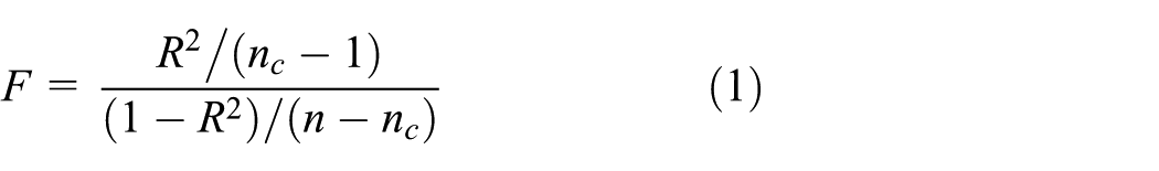
where

where n is the number of features (growth-determining SWC-EC-value pairs), ni is the number of the features in cluster i, nc is the number of clusters, nv is the number of growth-determining variables used to cluster features,
The two variables combined were used in the computation of the C-H index to select the optimal number of clusters (monitoring zones). The options M = 2, …, 15 were iteratively assessed for their effectiveness in dividing the trees into several groups (monitoring zones). As shown in Figure 1, the option M = 8 resulted in the highest C-H index, which indicated that it was most suitable for implementing ideal data collection if we partitioned the 10-year-old date palm trees into eight monitoring zones.
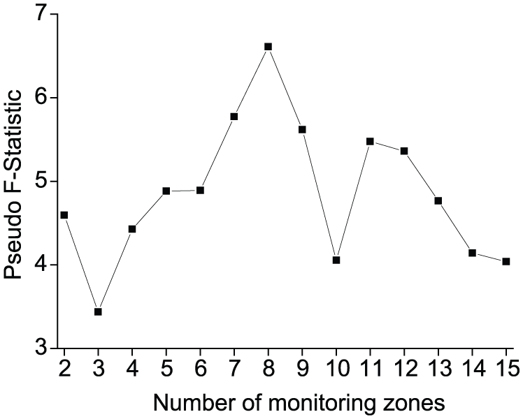
C-H index versus number of monitoring zones.
Next, spatial k-means was applied to partition the entire orchard into spatially contiguous monitoring zone. The spatial constraint was set as eight nearest neighboring trees. As a result of delineating monitoring zones, Figure 2 depicts the distribution of all monitoring zones and tree number belonging to each zone. The trees’ coordinates were pre-defined and fixed, depending on the orchard layout.

Output of delineating monitoring zones.
Determining required sensors number
For the sensor distribution with more than one growth-determining variable, the key question is to determine how many sensors are needed to simultaneously meet the individual accuracy requirement of all the variables. For this purpose, we separately calculated the number of the required sensors for each variable which could meet with a target accuracy and confidence level. Then, the number of the deployed sensors was determined considering the economic cost in addition to the data accuracy requirement.
Assume that one considered growth-determining variable, for which
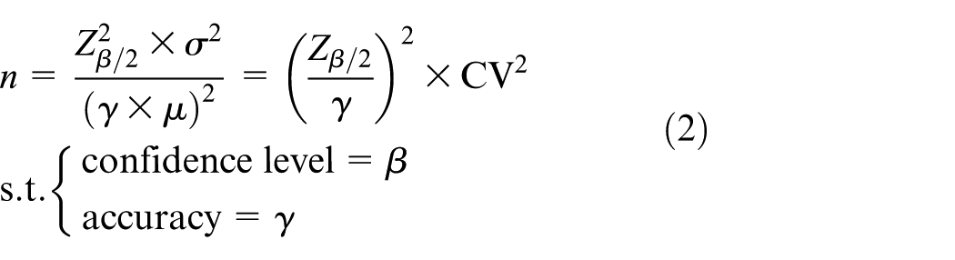
where
From the probability theory, the following mathematical relationship held 23

Apparently, the probability was
Here, we chose the expected confidence level 95% and the expected accuracy 90%. This meant that the calculated number of monitoring points aimed to meet the requirement of estimating the values of any growth-determining variable to be within 10% of the true mean with a 95% probability. Accordingly, the number of the required monitoring locations was calculated as follows
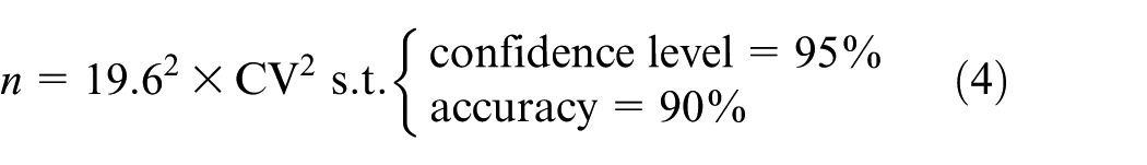
From the CV of SWC and EC tabulated in Table 1, the number of required monitoring locations for SWC and EC was 15 and 19, respectively.
Afterward, we took the criterion into consideration to further determine the sensor number for each monitoring zone: (1) the collected data complied with the expected accuracy, and (2) each cluster should be monitored by at least one sensor
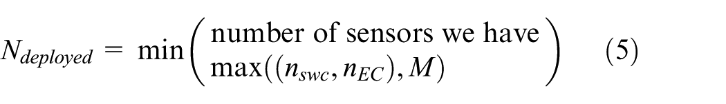
where M is the number of monitoring zones,
As shown in formula (5), the number of deployment sensors was determined by three factors: the number of sensors we had, the required numbers of the sensors and monitoring zones. The criterion could be modified arbitrarily depending on the practical data quality requirement, the cost we could afford, and the attention we paid to interesting variable. In our case, we assumed that we had in hand as many sensors as needed. Thus, 19 sensors are finally determined to be deployed.
Distributing sensors for monitoring zones
It is natural to imagine that there are differences in the tree number among these monitoring zones. We chose the weighted average of the tree number and the CV values of the two growth-determining variables as the deployment factor for each monitoring zone. It should be noticed that there were totally three variables to be considered in our case. To deal with the multi-variable problem, an additional weight, denoted as
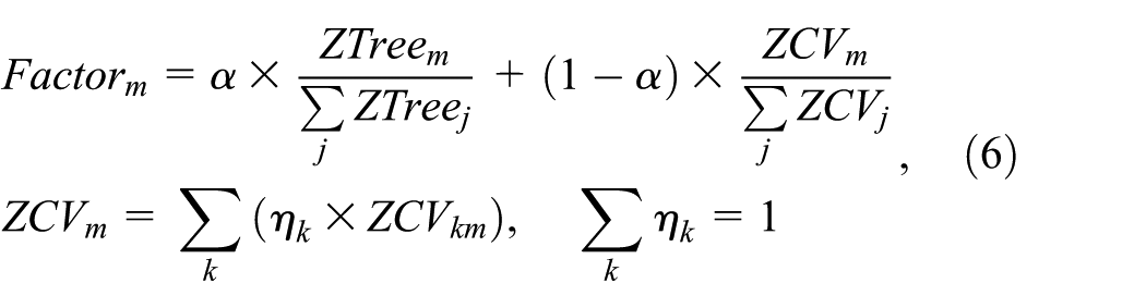
where
Finally, the required 19 sensors were distributed into eight monitoring zones using the formula (7) based on the weighted deployment factors of each monitoring zone

In our case,
The distribution of sensor number for eight monitoring zones is tabulated in Table 2 to evaluate the effectiveness of the proposed weighted factor method.
Sensor distribution for eight monitoring zones.
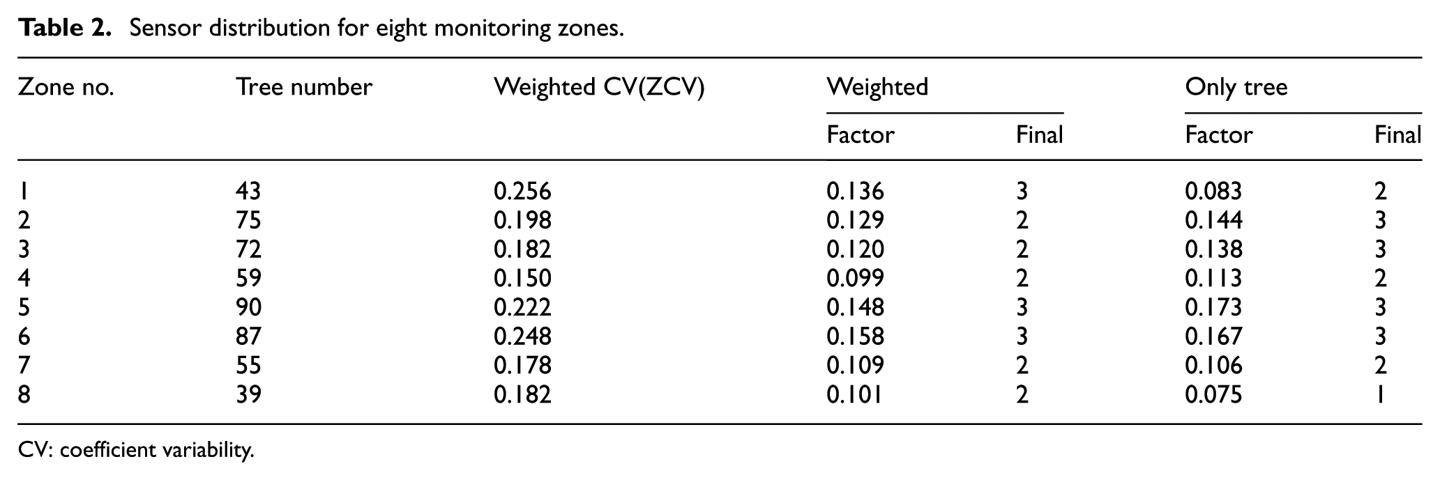
CV: coefficient variability.
As can be seen in Table 2, the weighted method has significant advantages over the other method. For instance, the weighted method assigned one more sensor for the no. 8 zone than only-tree method did. As a matter of fact, the weighted method was capable of offering better data collection solution compared with the only-tree method. This conclusion was drawn from the fact that the no. 8 zone did have a rather high CV. It was demanding to install more sensors for collecting the data of the two interesting variables due to the dynamic and random characteristics of SWC and EC. Additionally, the weighted method provided a good opportunity of reducing the cost of the relays or nodes, by taking into consideration the zone scale that was essential for networking WSNs. Above all, the weighted method helped in achieving a good tradeoff between networking and data collection quality. In contrast, the only-tree method had shortcomings in collecting data since it was merely dependent on the number of the trees, neglecting other important growth-determining factors.
Received signal strength distribution within the 10-year-old orchard
The same instruments and measurement scheme, used in our previous work, 13 were employed to investigate the wireless signal distribution within the 10-year-old orchard. The transmitter and receiver were XBee Pro® S2B modules, implementing the ZigBee protocol stack, and operating at the ISM 2.4 GHz frequency band. The modules were also used to construct WSN. The power output of the transmitter ranged from 6 to 12 dBm, including five levels. The modules made physical connections with two notebook computers through USB extension cables. The XCTU v6.2.0 software was employed to take the readings of received signal strength indicators (RSSI).
Similar to the scenario in Rao et al., 13 the antennas were attached to the palm trunks at a distance of 0.05 m away and at several typical heights. The antennas were attached to the trunks because the cultivation and harvest usually were greatly dependent on machinery, and the farmers expect sensor deployment not to disturb their machinery operation. The distance of 0.05 m was determined based on the need for machinery operation and preliminary received signal strength tests. 13 It is worthwhile to emphasize that the heights, slightly lower than the crown base, were the preferred locations for the placement of the sensor antennas since there were length limits for the cables of some commonly used sensors, such as sap flow sensors, soil properties, and fruit size. In our case, the chosen height for antenna placement was 2.0 m, slightly below the crown bottom, which was a tradeoff between the sensor cable length limit and wireless signal propagation condition.
Two sets of measurements were conducted. The first measurement set was made along the lines, except the boundary lines. The objective was to estimate the reliable communication distance when the antennas were placed at the chosen height on trunks within the target 10-year-old orchard. It was observed that the RSSI was approximately equal to −93 dBm when the Rx antenna was placed at 117 m (13th tree) away from the Tx antenna, in which the packet loss occurred. The second measurement set was conducted to reveal the received signal strength distribution based on the chosen placement height in the target orchard. A Tx antenna was attached to a tree at such distance of 0.05 m away from the trunk at the chosen height. Moreover, an Rx antenna was placed closely to other trunks within the target orchard, following the two criteria: 13 (1) it was perfect to provide clear line of sight between Tx and Rx antennas, at least making the Rx antenna face the Tx antenna, and (2) it always was beneficial to keep the space adjacent to two antennas as clear as possible along the straight line on which the Tx and Rx antennas lay.
As shown in Figure 3, the rows/columns were introduced for making it clear to describe the locations of other trees relative to the tree attached by the Tx antenna. Moreover, the following assumptions were made. (1) The lines in horizontal direction were called as rows; moreover, the row containing the Tx antenna was referred to as Row 0. (2) The vertical lines were called as columns, and the column including the tree with the Tx antenna was Col 0. The columns were denoted as Col, in particular, Col 0 to Col 13, from left to right. The column direction toward which the trunk side with the Tx antenna faced was negative; on the other contrary, the opposite column direction was positive. The Rx antenna was gradually moved tree by tree, up to 13 trees away from the Tx antenna along the row, whereas the Rx antenna was moved up to 2 trees away from the Tx antenna along the positive columns since the received signal strength of the positive rows except Row 1 was rather weak. 13 The Rx antenna was moved up to seven trees away along the negative columns to make it easy for understanding the signal distribution at a large scale. To make the contour smoother, the RSSIs were calculated employing the logarithm model. Meanwhile, some reasonable measurements that seemed abnormal were reserved. The interested reader can be referred to the literature. 13
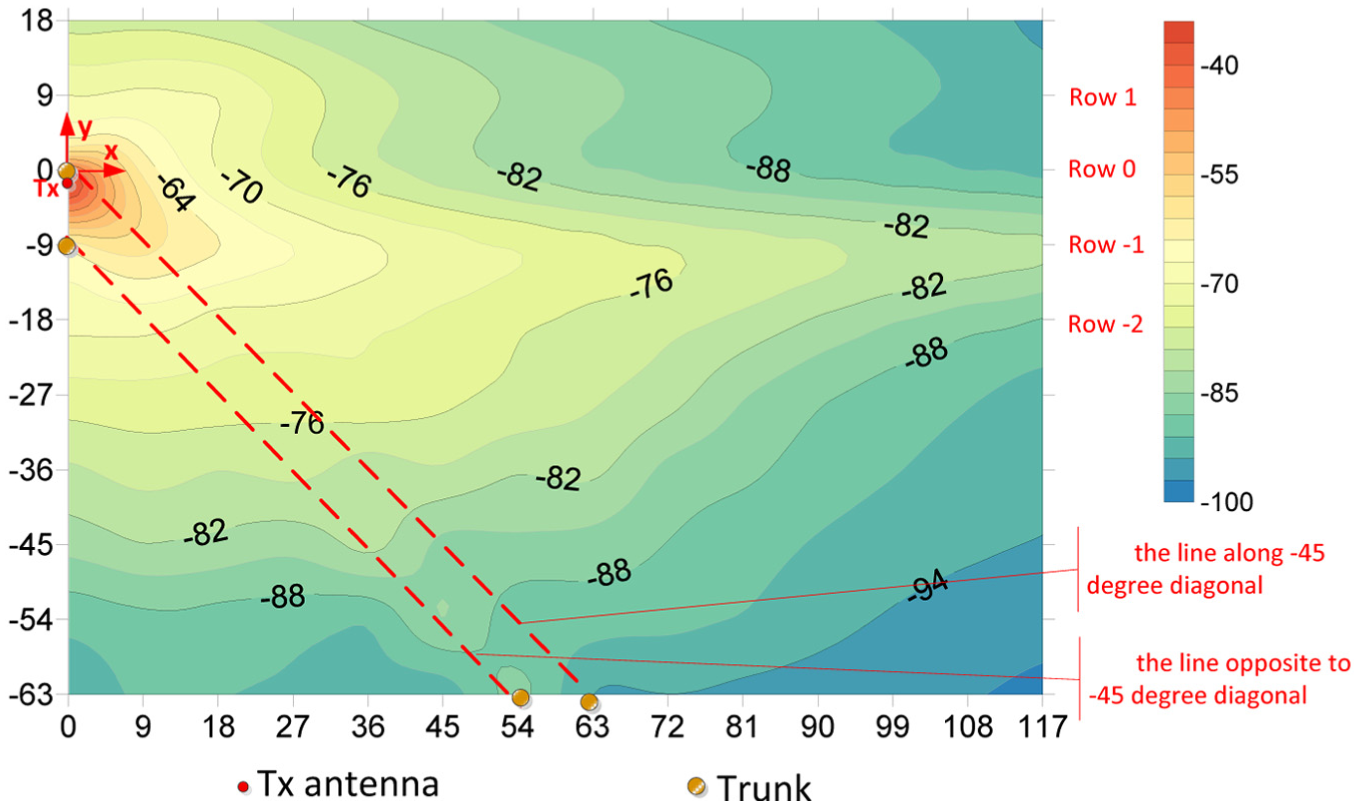
RSSI contour map of 14 × 10 trees with tree distance of 9 m in the 10-year-old orchard.
From Figure 3, the guidelines for antenna installation could be drawn. Generally, the preferred trunks for placing Rx antennas were located in Row −1. Rows 0 and 1 were the second choices for antenna placement. The third option was the line that was exactly opposite to the −45° diagonal. The fourth option would be those trunks in the direction toward which the trunk side with the Tx antenna faced. After carefully analyzing the measurements, it was discovered that there was an approximate numerical relationship among the reliable communication distances along Rows −1, 0, 1 and the line opposite to the −45° diagonal in the target orchard. In order to help in networking, the number of trees was used as a metric to compare the numerical relationship among the reliable communication distances of the preferred rows/line for antenna placement. More specifically, suppose that the reliable communication distance along Row 0 is D, then the reliable distance along Row −1 was about 1.4D, 1.2D along Row 1, and 0.6D along the line opposite to the −45° diagonal. Moreover, it was observed that the maximum reliable communication distance was 13, 15, 17, 19, and 22 trees, respectively, when the transmitter worked at its strongest transmit power. And the same numerical relationships of the reliable communication distances between three preferred choices held when the transmitter worked at five transmit power levels.
Note that we introduced the expressions, such as rows, diagonal, and lines (excluding the lines of sight), to help in describing the location relationships among the trunks with the Tx and Rx antennas attached. As for the selection of trunk side, the following criteria were taken into consideration: (1) it was perfect to provide clear line of sight between Tx and Rx antennas, at least making the Rx antenna face the Tx antenna; and (2) it always was beneficial to keep the regions adjacent to two antennas as clear as possible along the straight line on which the Tx and Rx antennas lay. It should be mentioned that the drawn guidelines aimed to determine the placement of the neighboring pairs of Tx and Rx antennas. This made it possible to implement flexible networking in practice since the proposed guidelines helped in offering a variety of antenna placement topologies in which the inter-node communications were maintained.
Joint deployment and discussion
Joint deployment practice
The flowchart of the joint deployment is shown in Figure 4. To ensure the fault tolerance of the system, all nodes in a WSN must have a minimum of 2-connectivity. In our case, the number of nodes was constant, and so was the number of monitoring zones in which the sensors were located and pre-determined resulting from the sensor distribution strategy in section “Sensor distribution strategy.” Therefore, the joint deployment of sensors was to select specific trees installing sensors in the monitoring zones and to ensure all nodes enjoyed at least 2-connectivity. Moreover, there were some additional constraints: (1) to prolong the network lifetime, all sensor nodes should work in as low energy consumption model as possible, and (2) the edge trees should first be eliminated from the candidates of the sensor placement. The condition of terminating the joint deployment calculation involved two aspects: (1) the minimization of power consumption and (2) 2-connectivity guarantee of all sensor nodes.

Flowchart of joint deployment.
Figure 5(a) shows one feasible deployment solution, in which it was achieved that all nodes work in the lowest transmission power and all of them had 2-connectivity. In field, as shown in Figure 5(b), we used Arduino Mega mainboards, XBee Pro® S2B modules, integrated with several interface and peripheral modules, to develop 19 wireless sensor nodes. Each deployed wireless node was connected to several types of sensors, such as soil moisture and EC, sap flow rate, frond elongation, and fruit size.

Feasible deployment solution and in-field realization: (a) one feasible deployment solution and (b) practical in-field deployment.
The WSN started to operate on 10 August 2015. The sensor nodes were powered by solar electricity. This battery was the rechargeable li-ion with a capacity of 7.2 AH. The wireless sensor nodes launched a round of data packet collection and transmission every 30 min. The coordinator was powered by electricity grid. During the operational observation of consecutive 30 days, none of the sensors underwent any working and power supply failure even though there were several overcast days. All nodes maintained at least 2-connectivity all the time. The packet delivery ratio reached over 97.34%. This demonstrated the effectiveness of our network deployment solution.
Data demonstration and discussion
Gathered data were really helpful for understanding the environmental and tree growth–related information in the date palm orchard and further guiding the daily orchard production management. It was witnessed that there were significant differences in the range among the same types of data within eight monitoring zones; however, the same types of data exhibited similar variation trend. Three groups of typical data, that is, sap flow, SWC, and frond elongation, are presented to demonstrate the effectiveness of the deployed WSN. In order to clearly illustrate the results of data gathering, we focus on the data from three types of sensors deployed within 1, 2, 3, and 4 zones, that is, four of eight monitoring zones, in the 10-year-old orchard during the time from 1 September 0:00 to 9 September 23:00, 2015.
The sap flow rate is a good representative indicator of whether the date palm trees are suffering water stress since the sap flow sensor implements internal continuous water status and flow measurements. Figure 6 depicts the sap flow rate from four sap flow sensors deployed within four different monitoring zones. As shown in Figure 6, the sap flow rates had the same variation trend as the reference evapotranspiration (ET0) that was obtained from a close meteorological station. This reasonable result demonstrated that the deployed WSN was capable of providing effective data collection. Moreover, the measurement is meaningful for achieving precise irrigation schedule in the future. Generally, the water consumption by the crop could be derived from the reference evapotranspiration (ET0) multiplied by an empirical crop factor (Kc). However, there are temporal variations in Kc with season and phenological stage. 11 As a result, at the early stage of WSN deployment, the trend difference between sap flow rate and ET0 can roughly help in improving irrigation schedule. 24 Fortunately, the crop factor (Kc) of date palm trees can be determined through investigating the long-term monitoring data. In the future, the precise irrigation amount can be calculated based on the previously experimentally obtained parameters.

Comparison of sap flow rate and ET0.
Figure 7 illustrates the SWC for four monitoring zones. Four zones had the similar variation trends of SWC. And the four curves of SWC reached their peaks at the noon, and then kept decreasing till the nighttime. This phenomenon complied with the irrigation schedule and plant physiology. The irrigation operated from 7:00 to 13:00. Therefore, there was high water content in the soil during the irrigation time. On the contrary, the SWC was becoming less and less after noontime due to the suspended irrigation and the root water uptake of date palm trees.

Soil water content versus time.
As for the frond elongation rate, it is a very important indicator of the growth and health of date palm trees. Figure 8 presents the frond elongation rates from four frond elongation sensors deployed within four different monitoring zones. As can be seen in this figure, the frond elongation rates reached peaks almost at the midnight of 0:00, then decreased to the lower point (almost zero) at the midday of 12:00. From the comparison of Figures 7 and 8, it is observed that there was exactly opposite variation trend between SWC and frond elongation rate. It is worthwhile to emphasize that the opposite trend was consistent with and truly reflected the physiological feature of date palm tree. In the daytime, the date palm tree maintained a slow growth rate due to the higher transpiration demand. In contrast, the tree grew faster due to the lower transpiration demand during the nighttime.

Frond elongation versus time.
Note that there were some abnormal values in Figure 8, for example, some points had negative values; meanwhile, some values were greater than 6. The phenomena should be ascribed to the sensor faults. In the future, we will try to fix these kinds of problems and further improve the availability of our WSNs.
Conclusion
During this study, an experimental in-field sensor network was developed for monitoring a 10-year-old date palm orchard in real time. Within the system, the required number and placement of sensors were determined by considering the data accuracy requirement, delineating the orchard into several monitoring zones, and combining the tree number with the CV of two growth-determining soil variables in the monitoring zones. In addition, the networking was realized by synthesizing the wireless signal strength distribution. Practical operation demonstrated the effectiveness of the experimental in-field sensor network. As the first WSN deployment considering the spatial variability, together with the wireless signal distribution, it lays one fundamental reference for future precision agriculture although its functionality needs to be further confirmed and extended.
Footnotes
Acknowledgements
The authors would like to express their gratitude to Naftali Lazarovitch, Yuval Shani, and Jingbo Zhen for their invaluable assistance and support, and special thanks to the growers for allowing us access to their orchards.
Academic Editor: Maio Jin
Declaration of conflicting interests
The author(s) declared no potential conflicts of interest with respect to the research, authorship, and/or publication of this article.
Funding
The author(s) disclosed receipt of the following financial support for the research, authorship, and/or publication of this article: The subject is sponsored by the National Natural Science Foundation of P.R. China (Nos 61203217, 61402013, and 61572261), the Introduction and Innovation of International Advanced Agricultural Science and Technology Program (Nos 2015-Z44, 2016-X34), the Natural Science Foundation of Anhui Province (No. 1608085QF126), the Scientific & Technological Research Project of Anhui Province (No. 1501031102), the Jiangsu High Technology Research Key Laboratory for Wireless Sensor Networks (No. WSNLBKF201506), the I-CORE Program of the Planning and Budgeting Committee, and the Israel Science Foundation (No.152/11).