Sage Journals: Discover world-class research

Abstract

In wireless sensor networks, node localization is the first operation after deployment, and the efficiency of localization can directly influence the performance of the wireless sensor network, so designing an efficient localization algorithm has been an important focus in wireless sensor network research. Currently, anchor-free algorithms are the focus of research in node localization because they have the advantages of flexible structure, low cost, high stability and good extensibility. In this article, related research studies of unique localization-, angle- and distance-obtaining methods are introduced, and existing algorithms are analysed. Based on the analysis of existing research, an anchor-free localization algorithm named ladder diffusion node localization algorithm is proposed, in which sensor nodes are located by directional diffused activation and acknowledgement packets with fixed energy. In ladder diffusion node localization algorithm, the time cost of localization is greatly reduced, the communication tasks in localization are allocated in a more balanced manner, and node locations are obtained mainly by rigorous computation instead of measurement, which can reduce transmission measurement error. Finally, the performance of ladder diffusion node localization algorithm is proved both in theory and by the simulation results of experiments.

Keywords

Wireless sensor networks global rigidity based on combined constraints uniqueness of localization ladder diffusion anchor-free algorithm

Introduction

Wireless sensor networks (WSNs) are one of the most important technologies in information science and can improve the ability to obtain information in harsh environments,^1–4 and they have broad application prospects in armillary, agriculture, industry and so on.^5–7 In WSNs, there are one or a few sink nodes and many sensor nodes. Sensor nodes monitor the target area and transmit messages, and sink nodes are responsible for collecting messages from all sensor nodes.^1,2 A sink node will be deployed in a specified spot, and it has limitless energy and powerful calculation and transmission capabilities; sensor nodes are randomly deployed in the target area, and their energy and calculation are limited by their volume.^3,4,7 According to the structural characteristics, algorithms for WSNs are much different than those designed for cable networks, and locating sensor nodes is one of the most representative algorithms in WSN research. When WSNs have been deployed, not all of the sensor nodes know their actual positions in the target area, and the adjacent relationships of all nodes cannot be established; however, it is not possible to equip every node with a localization device because of hardware cost, so node localization becomes necessary in WSNs.^8,9

There have been many research studies focusing on node localization, and the resulting algorithms can be divided into two categories: anchor-based algorithms^10–12 and anchor-free algorithms.^13–16 In anchor-based algorithms, several special nodes called anchors will be deployed in selected spots of the target area, and these anchor nodes have limitless energy and powerful calculation and are equipped with a localization device; classical anchor-based algorithms include SPA¹⁰ and CSPA.¹¹ In SPA, the nodes in the region with the highest density will be chosen as position reference group, and the node with the most neighbors will be set as the coordinate origin. By communication with the coordinate origin, other nodes will obtain their position. In SPA, too many communications are operated in the procedure of localization, which consumes much nodes’ energy and reduces WSN’s lifetime. In CSPA, all nodes will be divided to some clusters, and in every cluster, the operation as SPA will be operated. In CSPA, the speed of localization is accelerated, and the computational cost is relatively small; however, the clustering procedure in CSPA will also operate many communications, and the accuracy of localization is much influenced by the method of clustering. The advantage of anchor-based algorithms is that they have high localization accuracy; however, these algorithms have an obvious defect in that the flexibility of WSN deployment is greatly reduced because anchor nodes restrict the target area scope. To resolve this problem, many anchor-free algorithms have been proposed. In anchor-free algorithms, all sensor nodes will be located by communicating with other nodes, and by comparing with the signals’ source nodes, all node positions can be computed without any anchor nodes. The anchor-free algorithms are more flexible in deployment and less restrictive in structure, so more and more research studies have focused on anchor-free localization algorithms. However, in these algorithms, the procedure of localization is too complicated to be accomplished by a sensor node. In addition, the accuracy of localization is lower than that of anchor-based algorithms, such as the classical anchor-free localization algorithm AAFL. In AAFL, sensor nodes are clustered after being activated, and there is a boundary node in every cluster that is responsible for communicating with other clusters nodes and locating its member nodes; in AAFL, the distributed structure reduces the calculation burden of every node, but it leads to a decrease in localization accuracy. The introduction about AAFL motivated by the existing research, a new anchor-free algorithm named ladder diffusion node localization algorithm (LDLA) is proposed in this article with simple operation and high efficiency. In LDLA, every sensor node will be located by calculating its relative position with a sink node; just a few transmissions are needed in the entire procedure of localization, and the calculation of localization is not too complicated for sensor nodes. To compare the performance of LDLA with other localization algorithms, a series of experiments is designed with a unified model of WSNs and a classical error generation method, and the comparisons used in these experiments are mainstream ones, such as average node residual energy, localization error and the ratio of activated nodes after a certain period. These comparisons can generally and fairly compare different algorithms in the same simulation.

The rest of this article is organized as follows: in section ‘Related works’, the related works are introduced; in section ‘The design of LDLA’, the design of LDLA is proposed in detail; in section ‘The proof of LDLA’s performance’, the performance of LDLA is proved in theory and compared with other algorithms by experiment; finally, the contributions of this article are concluded.

Related works

The theory of unique localization

In the procedure of localization, the necessary information includes the adjacency relationships among all nodes and the distances and angles between each pair of nodes. In WSNs, however, sensor nodes are numerous, and all nodes are randomly distributed in the target area, so the adjacency relationship of every pair of nodes is hard to discover, and thus, the uniqueness of node localization computed by limited information cannot be ensured.¹⁷ There have been some theories proposed to judge the uniqueness of node localization in WSNs: rigidity and global rigidity in frameworks, the coordination of formations of autonomous agents and combinatorial rigidity in frameworks.^18,19 In these theories, the key idea is that the structure of a WSN should be satisfied by the global rigidity framework, in which the distribution of sensor nodes should be satisfied by the connectivity of the rigid graph.²⁰ To accomplish this judgement, a large number of communications between sensor nodes and many complicated calculations should be executed, which would incur a large hardware burden for the sensor nodes. Meanwhile, for the distributed structure of a WSN, the global connectivity is hardly judged by any parts of the sensor nodes. Based on this research, a new concept of global rigidity based on combined constraints is proposed to judge the uniqueness of localization.²¹ In this theory, under the premise that angles and distances between nodes have been obtained, if every node has direct relations with at least three other nodes, the distribution of the WSN can satisfy the global rigidity in the framework, and all of the nodes can be located uniquely. If none of the nodes would ever be moved after they are deployed, the restrictive condition of the global rigidity in frameworks based on combined constraints can be modified, as every node needs just two direct and different neighbour nodes.

The method of localization

To locate sensor nodes in WSNs, the angle and distance from each sensor node to a sink node are necessary information. Angle-measuring equipment has been invented with low cost and high accuracy and is now widely applied in sensor nodes because this equipment can also help decide the transmission direction when sending messages, and now most localization research studies use the measuring equipment to obtain the angle information. The errors of angle measurement are generated by hardware, which can be estimated by a statistical method. The research studies of localization have been focused on how to obtain the distance information of nodes, and there have been many methods proposed. Received signal strength indication (RSSI), time of arrival (ToA) and time difference of arrival (TDoA) are frequently used methods for measuring the distance between nodes.²² In RSSI, a packet is sent by the source node with a fixed energy, and when the target node receives this packet, the distance from the source node to the target node is computed according to the decreasing degree of the packet’s signal. By this method, the distance can be obtained with a small extra hardware burden, and the method is easy to accomplish in WSNs; however, the performance of RSSI is greatly influenced by the transmission environment, and the measurement error is large. In ToA, the source node is synchronized with the target node, and the distance is computed by the period of packet transmission based on the speed of radio waves; however, this method is hard to accomplish given WSNs’ distributed structure. In TDoA, the source node should not synchronize with the target node, there are two packets transmitted by different transmission speed modes, and the distance is computed according to the time difference between these packets. TDoA is fit for application in distributed structures, but it needs additional hardware to achieve its results, so it is not a good choice for WSNs. According to the existing research, the accuracy and hardware cost are two key factors when designing the distance-measuring method in WSNs.

Based on the information regarding the angles and distances among sensor nodes, localization algorithms can be designed, and there are currently two types of algorithms: anchor-based ones and anchor-free ones. In anchor-based algorithms, sensor nodes can be accurately located, and the packets exchanged between nodes are few, with noncomplex calculations; however, anchor nodes restrict the flexibility of WSN deployment in the target area, so it is mainly used in small-scale WSNs.^10–12 In the current research, anchor-free algorithms are the focus. In anchor-free algorithms, there are no anchor nodes, all nodes have the same capability of transmission and calculation, and nodes are located by communicating with other nodes, in which the distance and angle can be computed. In anchor-free algorithms, the deployment of WSNs can be more flexible than anchor-based ones because there are no restrictions on the distribution of anchor nodes, and these algorithms can be used in large-scale WSNs, which are more common in WSN applications.^13–17 However, existing anchor-free algorithms have obvious defects: the calculation of localization is too complex to be efficiently accomplished by sensor nodes, too many communications are performed in the localization procedure and the accuracy of these algorithms is lower than that of anchor-based algorithms.^23,24

Based on the analysis of related works, the localization algorithm for WSNs should satisfy the demand of the unique localization theorem, the extra hardware burden should be minimized, and the calculation and communication in localization should be as small as possible. In addition to these demands, the localization of all nodes must be positioned as accurately as possible.

The design of LDLA

In this section, a simple but accurate anchor-free localization algorithm named LDLA is introduced in detail. LDLA is designed based on our previous research in Qu et al.,²⁵ but it is more efficient because in LDLA, sensor nodes are activated by the method of directional ladder data diffusion, and all sensor nodes are identified by their IDs, which reduces communications and improves the accuracy of localization. In addition, the localization system is better satisfied with a global rigid frame based on combined constraints. The entire procedure of LDLA is organized as follows: first, some activation packets will be broadcast by a sink node; second, if a sensor node receives an activation packet, this node will relay this packet by the ladder diffusion method, and meanwhile, it will provide feedback to the source node via an acknowledgement packet; finally, according to the packets received from source nodes and neighbour node positions, every sensor node can adjust its coordinate system to a unified one, a list storing neighbouring nodes will be established in each node, and the node’s relative position and absolute position can be calculated.

The main idea of LDLA

A sink node collects messages from all sensor nodes, so it acts as the coordinate origin of the entire localization system in LDLA. Because the sink node has limitless energy and powerful transmission capability, it transmits various activation packages by broadcasting with fixed energy, and the structure of the packet is as defined in Table 1. In Table 1, level indicates the hop number from the sink node to the node sending the packet. There are three packet types: Act, an activated packet; Ack, an acknowledgement packet; Dat, a common data packet. If the packet type is Act, Dis means the distance from source node to sink node, and if the packet type is Ack, Dis means the distance from source node to ending node; Ang is the angle value, and it is set similarly to Dis; Ene is the energy used to send packets. Then, all sensor nodes that receive activation packets with a clear signal can be considered the one-hop neighbouring nodes of the sink node.

Table 1.

The structure of packet.

ID	ID of the source node
Pkt-typ	The type of packet (Act/Ack/Dat)
Level	The level of the current packet
Dis	The distance from source node to sink node/current node
Ang	The angle of source node to sink node/current node
Ene	The transmission energy of this packet

When a sensor node receives an activation packet from a sink node, it will compute the distance from itself to the sink node. At first, the radio channel signal energy attenuation is computed via equation (1), which is mentioned in Rappaport,²⁶ and in equation (1), P_r is the residual energy of the activation packet arriving at the current node, P_t is the initial energy of the activation packet departing the source node, G_r is the antenna gain in the sink node, G_t is the antenna gain in the receiving side node, λ is the wireless signal wavelength and the distance the packet has been transmitted is D. According to equation (1), the distance from the sink node to the receiving side node can be computed by equation (2), and in equation (2), all of the parameters are the same as in equation (1). At the same time, the angle of these two nodes can be obtained by measure setting. The node that received activation packet from sink node would update this packet and relay it by the direction faraway sink node

P_{r} = P_{t} G_{t} G_{r} {(\frac{λ}{4 Π D})}^{2}

(1)

D = λ \sqrt{\frac{P_{t} G_{t} G}{16 Π^{2} P_{r_{r}}}}

(2)

In LDLA, a node that is not a one-hop neighbour of the sink node will not be activated until it has received no less than two activation packets from different source nodes, which is the demand of the combined constraints. When this node is activated, its position can be computed with different source node localization information, and at the same time, a list storing neighbouring nodes will be established in every activated node, and the list’s structure is shown in Table 2. This procedure will continue until all sensor nodes have been activated and located.

Table 2.

The structure of the neighbouring nodes list.

ID	The ID of a neighbouring node
Level	The level of this neighbouring node
Dis	The distance from the current node to the neighbouring node
Ang	The angle between the current node and the neighbouring node
Ene	The energy of the neighbouring node

The detailed design of LDLA

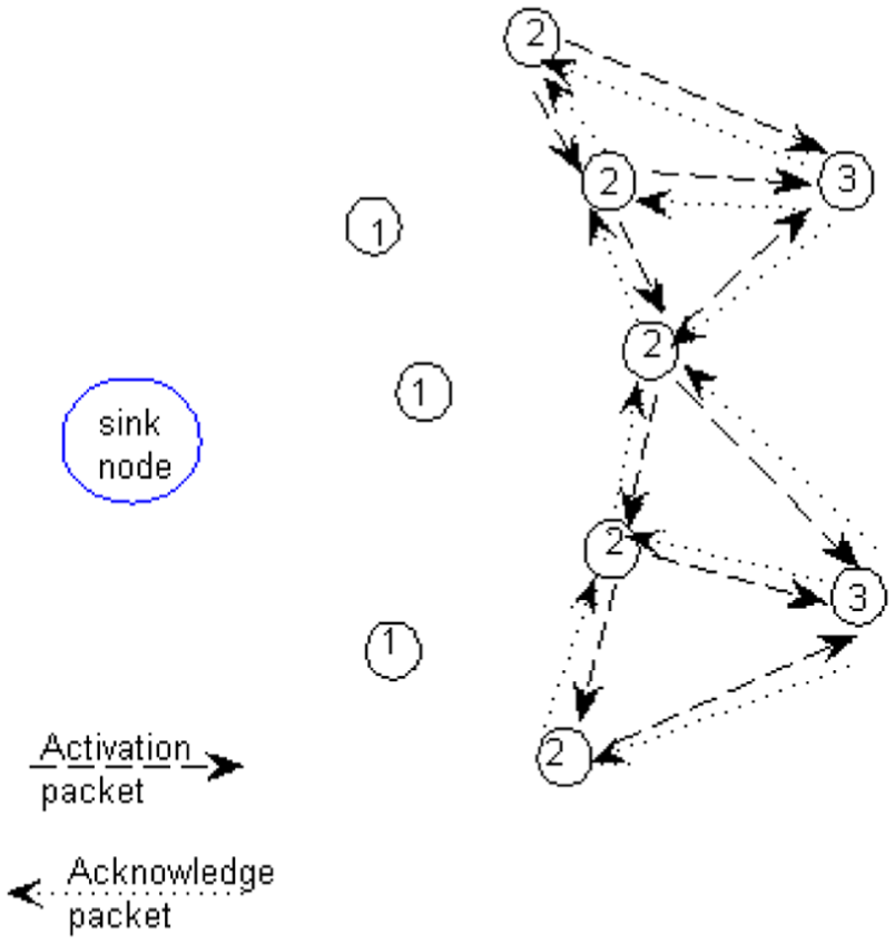
The first step of LDLA is to locate the one-hop neighbouring nodes of the sink node. The sink node broadcasts activation packets with fixed energy. The parameters of these packets are set as follows: the packet ID is set as 0, which means it is the sink node sending the packet; Pkt-typ is set as Act, which means that this packet is an activation packet; the level is set as 0, which means that the packet is sent by the sink node; the distance and angle of this packet are both 0; Ene is set as E₀, which means the packet is sent with energy value E₀; and the structure of this packet is as shown in Table 3. Sensor nodes that can receive these packets with a clear signal are regarded as one-hop neighbouring nodes of the sink node, and the illustration of this operation is shown in Figure 1.

Table 3.

The activation packet’s structure sent by the sink node.

Act

E ₀

Figure 1.

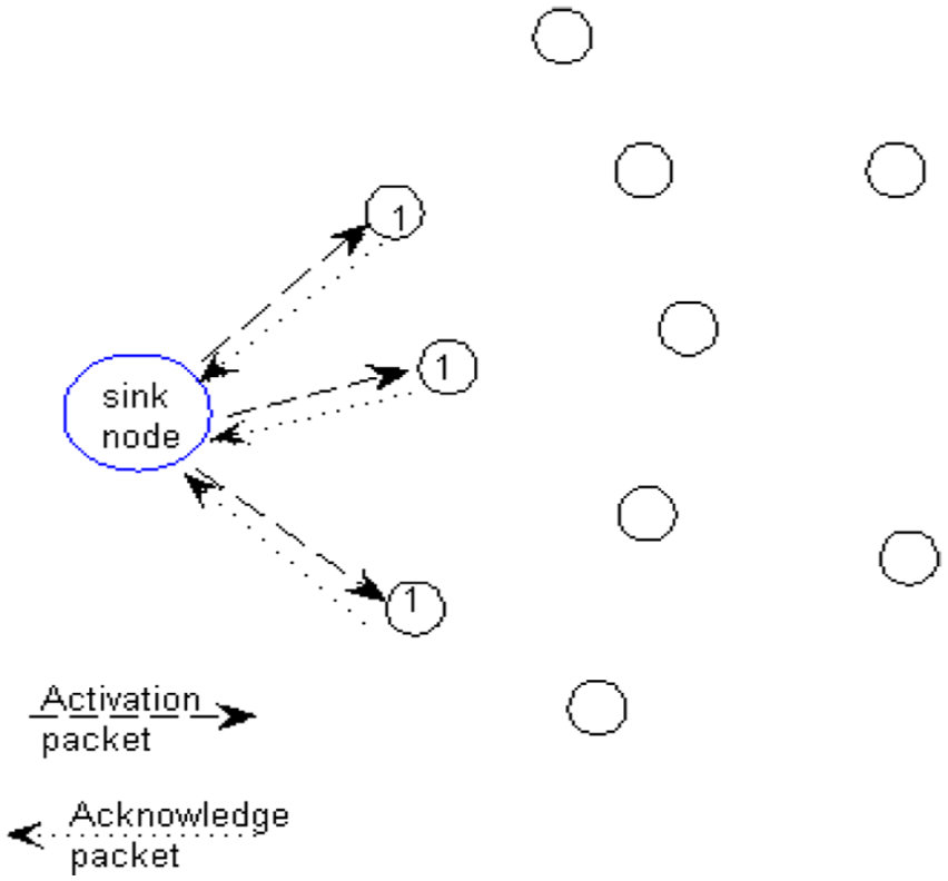
Activation one-hop neighbouring nodes of the sink node.

The one-hop neighbouring nodes compute the distance to the sink node according to the residual energy of the activation packet via equation (2) and then their coordinate origins are adjusted to unify with the sink node; the procedure is illustrated in Figure 2. In Figure 2, S is the sink node, A is a sensor node that can directly receive signals from the sink node, and the arrow with solid line means the direction of packet is sent, and the arrow with dotted line means the 0 degree angle direction in every node’s coordinate system, and there are three communications in Figure 2: in Figure 2(a), node A receives an activation packet sent by the sink node and the angle of this packet’s direction with 0 degrees angle direction of the coordinate system is α, but in the initial coordinate system of node A, this packet comes from the direction of θ; in Figure 2(b), node A has computed that the distance from itself to S is l_as and then it sends an acknowledgement packet with energy E₀ to S, whose structure is shown in Table 4; in Figure 2(c), S receives this acknowledgement packet, checks the distance and angle to node A as l_sa, computes the average value of the distance as l_A, updates the acknowledgement packet’s content as in Table 5 and feeds it back to node A; at the same time, node A is added to the neighbouring nodes list of the sink node, and node A adjusts its coordinate system via equation (3), in which γ is the angle that should be adjusted by node A. After this step, node A is activated, and the sink node is added to its neighbouring nodes list

α + θ + γ = 180 \circ C \Rightarrow γ = 180 \circ C - α - θ

(3)

Figure 2.

Obtaining the location of one-hop neighbouring nodes of the sink node.

Table 4.

Acknowledgement packet from node A.

Ack

l_as

E ₀

Table 5.

Acknowledgement packet from sink node.

Ack

l_A

E ₀

After the one-hop neighbouring nodes of the sink node have been activated, LDLA enters the next step. In this step, one-hop nodes set a transmission blind area, which is a sector that is 120°C wide, and the centre is the direction of the sink node. Then, one-hop nodes send activation packets to all directions except the blind area. Other nodes set the blind area by three steps: two sub-blind areas should be set, every area is a sector that is 120°C wide, and the centre is the direction of the source node. Then, the blind area is the union of these two sub-areas, and the sensor node just needs to send Act packets to the directions not in the blind area. The procedure is shown in Figure 3, and the packet structure is shown in Table 6. In Table 6, the level is set as 1, which means that the packet is sent by a one-hop neighbouring node of the sink node; the distance is set as l_A, which is the distance from node A to the sink node; the angle is set as α, which is the angle between node A and the sink node. In Figure 3, when a node receives an activation packet, it will compare the packet’s level with its own and then corresponding operations according to the comparison result should be executed: if the packet’s level is no less than its own and the source node has been in its neighbouring node list, the packet will be abandoned; if the packet’s level is less than its own and the source node has been in the list, the node receiving the packet will update its localization information and list content and send an acknowledgement packet to the source node as feedback, which is illustrated in Figure 4; if the node receiving the packet has not been activated, it will establish its neighbouring node list, and its coordinate system is adjusted to unify with the sink nodes, which is shown in Figure 5, but its localization information will not be computed until no less than two different activation packets have arrived and then it will feed back acknowledgement packets with its computing result to the source nodes, which is illustrated in Figure 6.

Figure 3.

Activation of next-hop nodes.

Table 6.

The structure of the activation packet sent by node A.

Act

l_A

E ₀

Figure 4.

Discovery of the neighbouring nodes.

Figure 5.

Adjustment of the direction of the coordinate system’s next-hop node.

Figure 6.

Calculation of the location of node C.

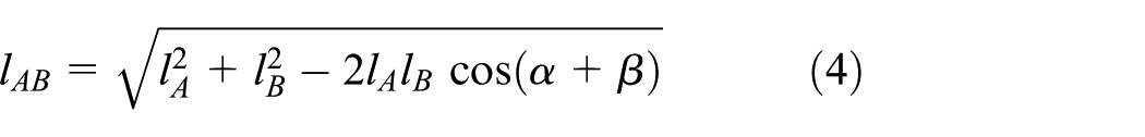
In Figure 4, node A and node B are both one-hop neighbouring nodes of the sink node, and node B receives an activated packet from node A, as in Table 6. Then, node B computes the distance from itself to node A via equation (4) and feeds an acknowledgement packet as in Table 7 back to node A. After this operation, node A and node B have both discovered the positions of each other and then they will update their neighbouring node lists by adding them as new items

l_{AB} = \sqrt{l_{A}^{2} + l_{B}^{2} - 2 l_{A} l_{B} \cos (α + β)}

(4)

Table 7.

The structure of the acknowledgement packet from node B.

Ack

l_BA

180°C − λ

E ₀

In Figure 5, node C is a sensor node that has not been activated, and it is not a one-hop neighbouring node of the sink node. Now, it receives an activation packet from node A as in Table 8 and then adjusts its coordinate system to unify with the sink node; the method is introduced in step 1. Node A plays the role of node S in this operation, and the acknowledgement packet from C is as in Table 9, and the acknowledgement packet from A is as in Table 10.

Table 8.

The structure of the activated packet from node A.

Act

l_a

E ₀

Table 9.

The structure of the acknowledgement packet from node C.

Ack

Null

E ₀

Table 10.

The structure of the acknowledgement packet from node A.

Ack

Null

E ₀

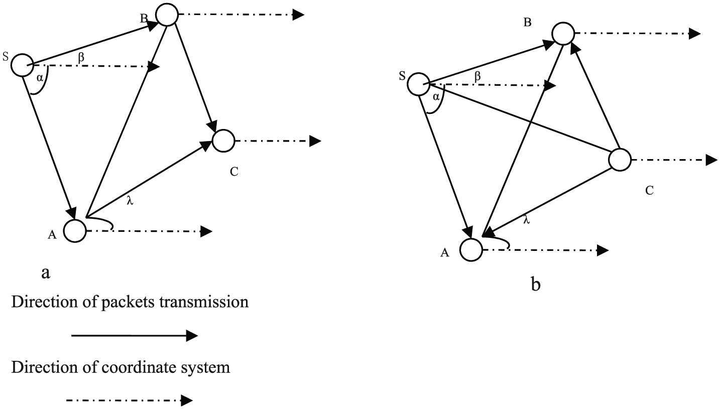
In Figure 6, node C receives two activation packets from different source nodes; these nodes can be of different levels, and they may not be neighbouring nodes; the packets’ contents are shown in Tables 11 and 12. Then, from these packets’ information, C can compute its position in the coordinate system of the sink node, and C sends acknowledgement packets to both A and B at the same time as feedback. In Figure 6(a), α is the angle of node A with sink node, and β is the angle of node B with sink node, and λ is the angle of node A with node C. Then node C can compute the distance from A to B according to equation (4) because the information needed by equation (4) has been in these activation packets, and both the angle between A and C and the angle between B and C can be measured. Then, C can compute the angles ABS and BAS with the distances l_A, l_B and l_AB by the trigonometric function formula in equation (5)

\begin{matrix} ∠ ABS = \arccos (\frac{l_{A}^{2} + l_{AB}^{2} - l_{B}^{2}}{2 l_{A} l_{AB}}) \\ ∠ BAS = \arccos (\frac{l_{B}^{2} + l_{AB}^{2} - l_{A}^{2}}{2 l_{B} l_{AB}}) \end{matrix}

(5)

Table 11.

The content of the Act packet from A.

Act

l_A

E ₀

Table 12.

The content of the Act packet from B.

Act

l_B

E ₀

By the result of the angle of equation (5) and the angles AOC and BOC, which can be measured by the measurement equipped in nodes A, B and C, the angles SAC and SBC can be computed by node C via equation (6), and O is the zero-degree direction line in every node’s coordinate system. Then, the angles BAC and ABC can be computed by equation (7)

\begin{matrix} ∠ S AC = 180 \circ - (180 \circ - ∠ AOC) - α = | ∠ AOC - α | \\ ∠ SBC = 180 \circ - (180 \circ - ∠ BOC) - β = | ∠ BOC - β | \end{matrix}

(6)

\begin{matrix} ∠ B AC = ∠ SA C - ∠ BA S \\ ∠ AB C = ∠ SB C - ∠ ABS \end{matrix}

(7)

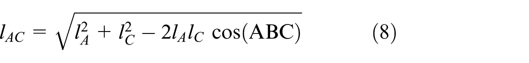
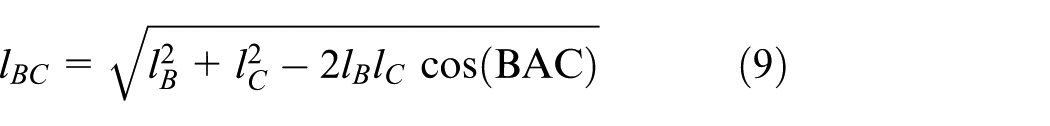
From the result of equation (7), both the distance from node A to node C, l_AC, and the distance from node B to node C, l_BC, are able to be computed by equations (8) and (9) based on the trigonometric function formula

l_{AC} = \sqrt{l_{A}^{2} + l_{C}^{2} - 2 l_{A} l_{C} \cos (ABC)}

(8)

l_{BC} = \sqrt{l_{B}^{2} + l_{C}^{2} - 2 l_{B} l_{C} \cos (BAC)}

(9)

From the value of l_AC or l_BC and the angle of SBC or SAC computed by equation (6), the distance from the sink node to node C, l_C, can be computed by equation (10)

l_{C} = \sqrt{l_{B}^{2} + l_{BC}^{2} - 2 l_{B} l_{BC} \cos (SBC)}

(10)

From the value of l_C and the value of l_BC (or l_AC), adding to the value of l_B (or l_A) from the activated packet, the angle of SCB (or SCA) can be computed by equation (11), and based on the result of SCB (or SCA) and the measurement value of the angle of BOC (or AOC), the angle between the sink node and node C, SCO, can be computed by equation (12)

∠ SCB = \arccos (\frac{l_{C}^{2} + l_{BC}^{2} - l_{B}^{2}}{2 l_{C} l_{BC}})

(11)

∠ SCO = ∠ SCB + ∠ BOC

(12)

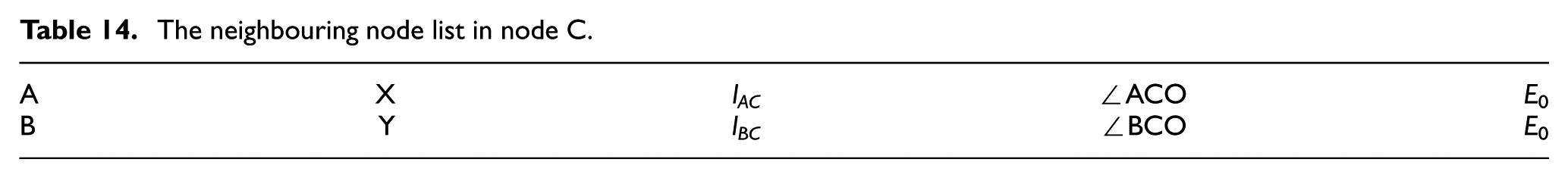
The pair value of distance l_C and angle SCO is the position of node C in the coordinate system of the sink node, the procedure of localization node C is end and the level of node C should be plus one based on the lesser one between node A and node B. Finally, node C feeds two acknowledgement packets back to A and B with its localization information, as in Table 13, and at the same time, C will establish the neighbouring nodes list and add node A and node B into this list, which is shown in Table 14.

Table 13.

The structure of the acknowledgement packet from node C.

Ack

l_C

∠SCO

E ₀

Table 14.

The neighbouring node list in node C.

A	X	l_AC	∠ACO	E ₀
B	Y	l_BC	∠BCO	E ₀

In step 3, as in Figure 7, the outer layer nodes will be activated and located, and the operation is the same as that introduced in step 2. However, in the target area of WSNs, there may be some isolated nodes that cannot receive any activation packets. To activate and locate these nodes, some applying packets will be broadcast by these nodes, and the packet’s structure is shown in Table 15.

Figure 7.

Activation of next-hop nodes and discovery of neighbouring nodes.

Table 15.

The structure of the applying packet of an isolated node.

Act

Null

E ₁

In Table 15, the packet’s type is set as Act, and the level is null, which means that this is an activation packet from an unactivated node with ID X, its localization information of distance and angle is null and its initial sending energy is set as E₁, which should be larger than E₀ to ensure that no less than two nodes can receive the packet. If a node receives this packet, it will feed back an acknowledgement packet with energy E₁, and node X will execute the operations as node C in step 2 when it has received no less than two acknowledgement packets from different nodes. Repeat this procedure until all isolated nodes have been activated and located.

The proof of LDLA’s performance

In this section, the performance of LDLA is proved. This section is divided into two parts: first, the uniqueness of localization of LDLA is proved by judging whether its structure satisfies the demand of uniqueness of the localization theorem; second, a series of experiments is designed, and LDLA is simulated for comparison with several existing typical localization algorithms to prove its localization performance.

The analysis of LDLA’s structure in unique localization theory

The algorithm proposed in this article is designed to be satisfied with the global rigid framework based on the theory of combined constraints. Combined constraints improve the rigidity of the framework, and in this framework, the set of edges can be described as B∪L. B is the set of edges that satisfy the angle constraint, and they are named the azimuth line; L is the set of edges that satisfy the distance constraint, and they are named the length line.²¹ The set of mixed edges is the intersection of the two edge types, and if there are more mixed edges in a network, its framework will be more likely to satisfy the global rigidity. It has been proved that if all node degrees are no less than 3, the framework satisfies the global rigidity. In Figure 8, a framework model with combined constraints is shown, and in this model, all node degrees are no less than 3 except node 6; however, node 6 has two length lines, but it also has an azimuth line, so it is a global rigidity framework. In Whiteley and Servatius,²¹ it was proved that, if all nodes are not mobile when they are deployed, the necessary and sufficient condition of global rigidity with combined constraints is that the degrees of all nodes in every sub-graph should be no less than 2.

Figure 8.

A global rigidity framework.

In LDLA, the communication channels can appear as the edges in combined constraints, and all packets sent in the localization procedure include both angle and distance information, so all communication channels can appear as mixed edges as B = L. In the localization procedure of LDLA, all nodes will not only receive activation packets but also receive acknowledgement packets, which include angle and distance information, so all node degrees can be ensured to be no less than 2. Based on the conclusion of the last paragraph, LDLA’s framework can satisfy the global rigidity with combined constraints, and the model is shown in Figure 9.

Figure 9.

Framework of LDLA.

The simulation model and standards

In this section, several classical localization algorithms are compared with LDLA, and the standards of comparison include accuracy of localization, efficiency of localization and energy conservation. To generally and fairly compare these algorithms, a model of WSNs is defined as follows:

All sensor nodes of a WSN are randomly distributed in the target area.

There is only one sink node in a WSN. The sink node is limitless in energy and is randomly located in the target area.

All sensor nodes have the same capabilities of calculation and communication.

Every node is equipped with angle measurement, and it can exactly measure the angle from the source signal to itself.

All nodes are not mobile after they are deployed, they can use proper energy to transmit information and the transmission direction can be accurately controlled.

The channel of transmission between two nodes is symmetrical, which means that the channel from node A to node B is the same as the channel from node B to node A.

The error in computing node positions follows the normal distribution N (0, σ²); the value of σ is set as 1 when computing distance and 1° when measuring angle, and then the error can be calculated by equation (13)

f (x) = \frac{1}{\sqrt{2 π}} e^{- 1 / 2}

(13)

Based on the model of WSNs, some standards are defined to generally compare the performances of localization algorithms, which are listed in the following.

Accuracy

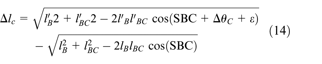
Localization accuracy means that the test error of computing should be as small as possible. According to Figure 2, the distance error of a one-hop neighbouring node with ID A is defined as (Δl_as + Δl_sa)/2, where Δl_as is the measurement error generated by node A and Δl_sa is the measurement error generated by the sink node; the angle error of a one-hop neighbouring node of the sink is Δθ, which follows equation (13). Then, the angle error of a node that is not a one-hop neighbour of the sink node with ID C is Δθ_c = Δθ_a + ε, where Δθ_a is the error of the last-hop node with ID a and ε is the error generated in node c. Then, the distance error of node c can be computed by equation (14) based on equations (8)–(10). In equation (14), $l'_{B}$ is the distance to the sink node including error, and $l'_{BC}$ is the distance from node B to node C including error, which can be computed based on equation (9)

\begin{array}{l} Δ l_{c} = \sqrt{{l^{'}}_{B}^{2} + {l^{'}}_{B C}^{2} - 2 {l^{'}}_{B} {l^{'}}_{B C} \cos (SBC + Δ θ_{C} + ε)} \\ - \sqrt{l_{B}^{2} + l_{B C}^{2} - 2 l_{B} l_{B C} \cos (SBC)} \end{array}

(14)

Based on equation (14), the error ratio of LDLA can be computed, and the localization errors of all algorithms compared in this article are computed by equation (15); in equation (15), (l_ir, θ_ir) is the real position value of node i in polar coordinates; $ω_{i}$ is the error ratio of node i; f(x_i) and f(y_i) are the positions of node i including error in the horizontal coordinates and vertical coordinates, respectively; $\bar{ω}$ is the average ratio of all nodes; and n is the number of sensor nodes. When the value of $\bar{ω}$ is larger, the accuracy of the localization algorithm is worse

ω_{i} = \frac{\sqrt{f^{2} (x_{i}) + f^{2} (y_{i})}}{\sqrt{{(l_{i r} \cos θ_{i r})}^{2} + {(l_{i r} \sin θ_{i r})}^{2}}}; \bar{ω} = \frac{\sum_{i = 1}^{n} ω_{i}}{n}

(15)

Efficiency

In this section, efficiency means that sensor nodes in WSNs should be fast and precisely located. Then, the time that it takes for localization should be as short as possible under the premise of localization accuracy. Thus, the standard of efficiency is set as the ratio of located nodes per unit time with relatively high accuracy.

Energy saving property

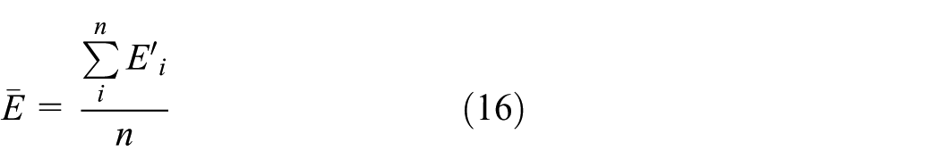
In WSNs, sensor nodes’ residual energy is limited, and if too much energy is used in the localization procedure, the WSN’s lifetime will be much reduced. In WSNs, the energy consumed in transmission is much higher than that in other operations, but many transmissions are needed for localization, so how to conserve energy is an important factor in improving localization performance. For the distributed structure of WSNs, the energy consumption of every node is unbalanced, so the localization algorithm should focus on balancing the residual energy of nodes, and the standards are defined as equations (16) and (17). In equation (16), $\bar{E}$ is the average residual energy of all nodes, n is the number of nodes and $E'_{i}$ is the residual energy of node i; when the result of equation (16) is larger, the performance of the algorithm is better. In equation (17), $Δ E$ is the difference between the maximum residual energy and the minimum residual energy; when the result is lower, the performance is better. The energy consumption formula for communicating is the typically adopted one, shown in equation (18), and in this equation, L is the length of transmission, d is the distance of transmission, E_El_ec is a hardware parameter of the energy consumption in the transmission channel, e_fs and e_m_p are hardware parameters of the energy consumption in amplifier operation and d₀ is a threshold of distance related to the node hardware: if d is less than d₀, the energy consumption is proportional to the quadratic d; if d is larger than d₀, the energy consumption is proportional to the biquadratic d

\bar{E} = \frac{\sum_{i}^{n} {E'}_{i}}{n}

(16)

Δ E = E_{MAX} - E_{MIN}

(17)

E_{TX} (L, d) = {\begin{matrix} L E_{Elec} + L ε_{fs} d^{2}, d < d_{0} \\ L E_{Elec} + L ε_{mp} d^{4}, d > d_{0} \end{matrix}

(18)

The simulation experiments

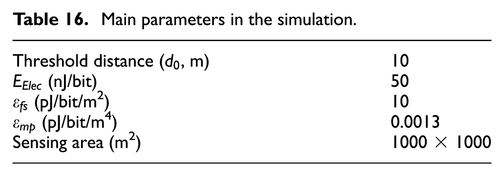
To compare the performance of LDLA with other algorithms, a series of experiments is simulated by MATLAB, and these algorithms include anchor-based algorithms, such as SPA¹⁰ and CSPA,¹¹ and anchor-free algorithms, such as AAFL.¹⁵ The main environment parameters of the simulation are shown in Table 16, and the hardware parameters in this simulation are set to popular values.

Table 16.

Main parameters in the simulation.

Threshold distance ( $d_{0}$ , m)	10
$E_{Elec}$ (nJ/bit)	50
$ε_{fs}$ (pJ/bit/m²)	10
$ε_{mp}$ (pJ/bit/m⁴)	0.0013
Sensing area (m²)	1000 × 1000

To generally compare the performance of localization algorithms, there are two types of experiments: one is the changing tendency of accuracy, efficiency and energy conservation with the increase in the number of nodes under the condition of fixed localization coverage; the other is the changing tendency of accuracy, efficiency and energy conservation with the increase in localization coverage under the condition of unchanged number of nodes.

In Figure 10, the changing tendency of localization accuracy with the increase in the number of nodes is shown under the condition that localization coverage is fixed at 90%. When the number of nodes is <200, SPA and CSPA have the best localization accuracy, and AAFL and LDLA are slightly worse than SPA and CSPA. When the number of nodes is >300, the calculation of SPA is too complex to obtain a result, the result of CSPA changes slightly and LDLA is better than AAFL. When the number of nodes is >400, the accuracy of CSPA begins to decline, and LDLA just changes slightly. When the number of nodes is >500, LDLA is slightly worse than CSPA, and AAFL is much worse than these two algorithms. It can be concluded that the accuracy of LDLA is not obviously lower than anchor-based algorithms, it is affected by the number of nodes much less than the others, and in relatively large-scale WSNs, LDLA’s performance is better than anchor-based algorithms.

Figure 10.

The error changing with nodes’ number.

In Figure 11, the changing tendency of localization time with the increase in the number of nodes is shown under the condition that localization coverage is fixed at 90%. When the number of nodes is 100, the time cost of LDLA is the least of all the algorithms, and SPA is the largest; CSPA and AAFL are almost the same, and they are less than SPA but larger than LDLA. When the number of nodes is 200, the time cost of SPA is obviously increased, the time cost of both AAFL and LDLA are increased to a certain degree and the time cost of CSPA is increased least of all; however, LDLA still has the lowest time cost. When the number of nodes is >400, SPA is not able to finish the localization procedure in the limited time, the time cost of both CSPA and AAFL are obviously increased and just LDLA can maintain a relatively low time cost. By this result, it can be concluded that LDLA has an obvious advantage in localization speed, and its advantage is more obvious in large-scale WSNs.

Figure 11.

The time cost changing with the number of nodes.

In Figure 12, the changing tendency of nodes’ average residual energy with the increase in the number of nodes is shown under the condition that location coverage is fixed at 90%. When the number of nodes is <200, AAFL has the best residual energy level, the residual energy level of LDLA is slightly lower than that of AAFL, and SPA and CSPA have the lowest residual energy levels. When the number of nodes is >200, the residual energy level of LDLA begins to be better than that of AAFL, the performance of CSPA is also close to that of AAFL and SPA cannot accomplish the localization procedure. When the number of nodes is >400, only nodes in LDLA have relatively high residual energy. In Figure 13, the changing tendency of the difference between the maximum residual energy and the minimum residual energy is shown under the same condition. When the number of nodes is <400, the energy consumed in LDLA can remain highly balanced, and the largest difference value is 17%; even when the number of nodes is 500, the largest difference value of LDLA is just 20%, which is much less than other algorithms. The energy balance performance of CSPA is the lowest of all; when the number of nodes is 350, the difference value is 50%, and when the number of nodes is 500, the difference value is 77%, which means that some nodes’ energy will be exhausted. SPA and AAFL are not prominent in energy balance performance either. Based on the results shown in Figures 12 and 13, it can be concluded that LDLA is the best in energy conservation performance, regardless of the scale of the WSNs.

Figure 12.

The average residual energy changing with the number of nodes.

Figure 13.

The difference in nodes’ residual energy changing with the number of nodes.

In Figures 14 –17, the performance changing tendency of all algorithms is shown under the condition that the number of nodes in the WSN is fixed at 250. Considering the application specialist of all algorithms, the node number is set as 250, and this scale of WSN is the most balanced station.

Figure 14.

The error changing with localization nodes’ ratio.

Figure 15.

The localization time changing with the activated nodes’ ratio.

Figure 16.

The average nodes’ residual energy changing with the activated nodes’ ratio.

Figure 17.

The difference in nodes’ residual energy changing with the activated nodes’ ratio.

In Figure 14, the changing tendency of localization accuracy with the increase in the ratio of located nodes to all nodes is shown. When the ratio of located nodes is between 50% and 70%, SPA and CSPA have the best localization accuracy, the localization accuracy of LDLA is slightly lower than those of SPA and CSPA and AAFL has the lowest localization accuracy. When the ratio of located nodes is between 70% and 80%, SPA is not obviously affected, the localization error of CSPA increases quickly, the increase in LDLA changes just slightly more than that of SPA and the localization error of AAFL is larger than that of LDLA but less than that of CSPA. When the ratio of activated nodes is >90%, it is too large for SPA to obtain the result, the localization errors of AAFL and CSPA are both obviously increased, and only LADA is not obviously affected. By this result, it can be concluded that the localization accuracy of LDLA is affected little by sensor node positions.

In Figure 15, the changing tendency of localization time with the increase in the ratio of activated nodes to all nodes is shown. When the ratio of activated nodes is between 50% and 70%, the time costs of CSPA, AAFL and LDLA are not too different, and SPA has a slightly higher time cost than the others. When the ratio is between 70% and 90%, the time costs of all algorithms are improved obviously except for those of LDLA, and SPA is still the most affected. When the ratio is 95%, the leading edge of LDLA is very obvious, and SPA cannot finish the localization procedure. According to this result, it can be concluded that LDLA can efficiently discover and locate the nodes far away from the sink node, and this can greatly expand the WSN application range.

In Figure 16, the changing tendency of nodes’ residual energy with the increase in the ratio of activated nodes to all nodes is shown. It can be seen that regardless of the ratio, the average residual energy of LDLA is the highest of all the algorithms, and with an increase in the ratio, the advantage becomes more and more obvious. In Figure 17, the changing tendency of the difference between the maximum residual energy and the minimum residual energy is shown. According to this figure, the energy balance of CSPA is the lowest, LDLA is the best and AAFL and SPA are in between. According to the results of Figures 16 and 17, it can be concluded that in this condition, LDLA has great advantages in energy consumption balancing and in improving the network’s lifetime.

Analysis of the experiments

Based on the results of the experiments, LDLA has advantages in localization accuracy, localization efficiency and energy conservation.

Localization accuracy

In LDLA, the procedure of localization is satisfied with the global rigid framework based on the theory of combined constraints, which ensures unique localization for every node. Then, in LDLA, just the sink node’s one-hop neighbouring nodes’ positions are measured, and other nodes’ distances to the sink node are obtained by computation. To reduce the measurement error, every one-hop neighbouring node communicates with the sink node three times to verify the measurement result and then any other nodes compute their positions based on the one-hop neighbouring nodes’ positions. By this means, the accuracy of LDLA is only slightly affected by the number of nodes. However, in other algorithms such as SPA, CSPA and AAFL, all sensor nodes’ positions are obtained by both computation and measurement, and the error consists of measurement error and calculation error; then, the accuracy of localization may decline with the increase in the number of nodes.

Efficiency

In LDLA, the procedure of localization is designed with a distributed structure, and all nodes just need to discover and communicate with their neighbouring nodes, which greatly reduces invalid operations and communications; meanwhile, the activation packets are transmitted by ladder directional diffusion, which ensures that invalid transmissions is greatly avoided, the localization time cost of LDLA is greatly reduced and the efficiency is improved. In other algorithms, there are many invalid transmissions in the localization procedure, such as SPA and AAFL, and many complex operations are executed to obtain position information, such as CSPA and AAFL; thus, these algorithms are less efficient than LDLA.

Energy conservation

In LDLA, there are several innovations used to improve the energy conservation: first, the directional diffusion method is used to replace the broadcasting method, reducing many transmissions and thus conserving much node energy; second, all packets are sent with relatively little energy instead of broadcasting with large energy; finally, LDLA adopts the distributed discovery nodes method, in which all nodes need not communicate directly with the sink node, but by layers of progressive method to discovery nodes from the inside to the outside, and the nodes’ energy consumption is more balanced.

Conclusion

The node localization problem is an important factor influencing WSN performance and applications. In this article, existing methods for measuring angles and distances in WSNs are introduced, and their advantages and defects are analysed. Based on the analysis of existing localization algorithms, a new distributed and anchor-free localization algorithm named LDLA is proposed based on ladder diffusion. In LDLA, rigorous calculation, instead of measurement, is used to obtain nodes’ positions, which greatly reduces the error of localization; the distributed procedure allocates localization tasks in all nodes in a balanced manner and then the localization process is relatively fast, and the energy consumption is more balanced. Finally, the performance of LDLA is proved both in theory and in experiments. With the extensive application of WSNs, more research studies regarding three-dimensional (3D) localization^27–31 have been proposed, and our future studies will focus on extending the proposed localization algorithm in 3D environments.

Footnotes

Academic Editor: Seong-eun Yoo

Declaration of conflicting interests

The author(s) declared no potential conflicts of interest with respect to the research, authorship, and/or publication of this article.

Funding

The author(s) disclosed receipt of the following financial support for the research, authorship, and/or publication of this article: This research is supported by the Natural Science Foundation of China under contract number 60573065 and the Science and Technology Development Plan of Shandong Province under contract number 2014GGX101039, and it is partially supported by the Natural Science Foundation of China under contract number 60903176.

References

Akyildiz

Sankarasubramaniam

. Wireless sensor networks: a survey. Comput Netw 2002; 38(4): 393–422.

Yick

Mukherjee

Ghosal

. Wireless sensor network survey. Comput Netw 2008; 52(12): 2292–2330.

Van der Werff

. 10 emerging technologies that will change the world. MIT’s Technol Rev 2003; 32(2): 33–49.

Misra

Reisslein

Xue

. A survey of multimedia streaming in wireless sensor networks. IEEE Commun Surv Tut 2008; 10(4): 18–39.

Rehman

Abbasi

Islam

. A review of wireless sensors and networks’ applications in agriculture. Comput Stand Inter 2014; 36(2): 263–270.

Oliveira

Rodrigues

. Wireless sensor networks: a survey on environmental monitoring. J Comm 2011; 6(2): 143–155.

Alemdar

Ersoy

. Wireless sensor networks for healthcare: a survey. Comput Netw 2010; 54(15): 2688–2710.

Patwari

Ash

Kyperountas

. Locating the nodes: cooperative localization in wireless sensor networks. IEEE Signal Proc Mag 2005; 22(4): 54–69.

Getting

. The global positioning system. IEEE Spectrum 1993; 30(12): 36–47.

10.

Capkun

Hamdi

Hubaux

. GPS-free positioning in mobile ad hoc networks. Cluster Comput 2002; 5(2): 157–167.

11.

Iyengar

Sikdar

. Scalable and distributed GPS free positioning for sensor networks. In: Proceedings of the IEEE international conference on communications (ICC’03), Anchorage, AK, 11–15 May 2003, pp.338–342. New York: IEEE.

12.

Mao

Fidan

Anderson

BDO

. Wireless sensor network localization techniques. Comput Netw 2007; 51(10): 2529–2553.

13.

Wicker

. Co-designed anchor-free localization and location-based routing algorithm for rapidly-deployed wireless sensor networks. Inform Fusion 2008; 9(3): 425–439.

14.

Jord

Jackson

. Operations preserving global rigidity of generic direction-length frameworks. Int J Comput Geom Ap 2010; 20(6): 685–706.

15.

Youssef

Agrawala

. Accurate anchor-tree node localization in wireless sensor networks. In: Proceedings of the IEEE IPCCC, Phoenix, Arizona, 7–9 April 2005, pp.465–470. New York: IEEE.

16.

Aaron

. LOCOMOTE: a simple anchor-free localization scheme for wireless sensor networks. In: Proceedings of the IEEE military communications conference (MILCOM’07), Orlando, FL, 29–31 October 2007, pp.1–7. New York: IEEE.

17.

Harter

Hopper

. A distributed location system for the active office. IEEE Network 1994; 30: 62–70.

18.

Whiteley

. The union of matroids and the rigidity of frameworks. SIAM J Discrete Math 1988; 1(2): 237–255.

19.

Eren

Belhumeur

Anderson

BDO

. A framework for maintaining formations based on rigidity. In: Proceedings of the IFAC, Barcelona, 21–26 July 2002, pp.2752–2757. Amsterdam: Elsevier.

20.

Molina

Alba

. Location discovery in Wireless Sensor Networks using metaheuristics. Appl Soft Comput 2011; 11: 1223–1240.

21.

Whiteley

Servatius

. Constraining plane configurations in CAD: combinatorics of directions and lengths. SIAM J Discrete Math 1999; 12(1): 136–153.

22.

Kulakowski

Vales-Alonso

Egea-Lopez

. Angle-of-arrival localization based on antenna arrays for wireless sensor networks. Comput Electr Eng 2010; 36(6): 1181–1186.

23.

Jordt

Baldwin

Raquet

. Energy cost and error performance of range-aware, anchor-free localization algorithms. Ad Hoc Netw 2008; 6(4): 539–559.

24.

Hamilton

Baxley

. Efficient node self-localization in large ad-hoc wireless networks using interlaced particle filters. In: Proceedings of the IEEE military communications conference (MILCOM 2011), Baltimore, MD, 7–10 November 2011, pp.780–785. New York: IEEE.

25.

Shu

Yang

. An energy efficient anchor-free localization algorithm for no-identity wireless sensor networks. Int J Distrib Sens N 2015; 2015: 595246.

26.

Rappaport

. Wireless communications: principles and practice. 2nd ed. Upper Saddle River, NJ: Prentice Hall PTR, 2001.

27.

Zhang

Liu

Jia

. Localization using joint distance and angle information for 3D wireless sensor networks. IEEE Commun Lett 2012; 16(6): 809–811.

28.

Saeed

Stojkoska

. Robust localization algorithm for large scale 3D wireless sensor networks. Int J Ad Hoc Ubiq Co 2016; 23(1–2): 1–10.

29.

Liu

Wang

Chen

. A novel wireless 3D localization method supported by WSN. Int J Online Eng 2013; 9(2): 9.

30.

Cardoso

Guidoni

Maia

. An energy consumption aware solution for the 3D localization and synchronization problems in WSNs. In: Proceedings of the 2014 Brazilian symposium on computer networks and distributed systems, Florianópolis, Brazil, 5–9 May 2014, vol. 90, no. 6, pp.376–385. New York: IEEE.

31.

Vanheel

Verhaevert

Laermans

. Pseudo-3D RSSI-based WSN localization algorithm using linear regression. Wirel Commun Mob Com 2015; 15(9): 1342–1354.

A simple efficient anchor-free node localization algorithm for wireless sensor networks

Abstract

Keywords

Introduction

Related works

The theory of unique localization

The method of localization

The design of LDLA

The main idea of LDLA

The detailed design of LDLA

The proof of LDLA’s performance

The analysis of LDLA’s structure in unique localization theory

The simulation model and standards

Accuracy

Efficiency

Energy saving property

The simulation experiments

Analysis of the experiments

Localization accuracy

Efficiency

Energy conservation

Conclusion

Footnotes

Declaration of conflicting interests

Funding

References