An improved incremental least-mean-squares algorithm for distributed estimation over wireless sensor networks

Abstract

Distributed parameter estimation problem has attracted much attention due to its important foundation of some applications in wireless sensor networks. In this work, we first investigate the performance tradeoff between existing incremental least-mean-squares algorithm and traditional steepest-descent algorithm from the aspects of initial convergence rate, steady-state convergence behavior, and oscillation, and present the motivations for improvements. Thereby we propose an improved incremental least-mean-squares distributed estimation algorithm that starts from the incremental least-mean-squares algorithm and works toward the objective of improvement on initial convergence rate and steady-state performance. The proposed algorithm meets the requirements of diminishing step size for wireless sensor networks without any increase in communication overhead and the mean stability condition is derived for a practical guideline. A target localization model in wireless sensor networks is used to illustrate the effect of the proposed algorithm. Simulation results confirm the performance improvement of our method, as well as the effectiveness of application in wireless sensor networks.

Introduction

An important function of sensor nodes in wireless networks is to collect the measurements (e.g. temperature, humidity, distance, and direction), which can be used to estimate the unknown parameter that users are interested in. Such estimation problem can be considered in many application scenarios of wireless sensor networks (WSNs), for example, target localization^1,2 and tracking, ³ determining the parameters of an auto-regressive (AR) model or moving-average (MA) model, ⁴ power spectrum estimation, ⁵ and distributed detection. ⁶

Depending on the modes of cooperation predetermined by network topology, centralized and distributed estimation schemes have been proposed. The centralized schemes rely on a fusion center (FC) or cluster head (CH) that is responsible to estimate the unknown parameter by gathering the measurements over the entire sensor network. As a popular solution, the distributed scheme does not require any fusion center, but allows each node to perform local estimation fusion by only collecting the information from its neighboring nodes. The global estimation task is distributed among the nodes and each node can converge to same mean-square-deviation (MSD) levels, thus avoiding the failure of FC and balancing network load.

Many distributed estimation strategies have been proposed, such as the consensus strategy,^7,8 the incremental adaptive strategy,^9,10 and the diffusion adaptive strategy.^11–13 The consensus strategy aims to reach the consensus estimate of the parameter through the limited interaction among the nodes and the consensus time iterations. Distributed consensus-based Kalman filtering algorithm that combines consensus strategy into the standard Kalman filter has been well used for sensor schedule ¹⁴ and localization of target. ¹⁵ Originating from the consensus strategy, the incremental adaptive strategy requires a ring topology like the Hamiltonian cycle,^16,17 where each node is visited exactly once per iteration. So that the local measurements and the results from previous node on cycle path are fused to generate the new estimate of current node by iteration algorithm (e.g. least-mean-squares (LMS) algorithm, steepest-descent algorithm, and Gauss–Newton algorithm). This mode of operation is fully distributed and results in the least amount of communications and power. The incremental optimization techniques have been used for distributed maximum likelihood estimation (MLE), ¹⁸ network design for shortest paths. ¹⁹ Unlike the incremental mode, each node in the diffusion adaptive mode collects the information from all its neighbors and aggregate them in the Adapt-then-Combine (ATC) way or the Combine-then-Adapt (CTA) way. ¹¹ This complex cooperative mode leads to a significantly higher communication cost but more robust to node and link failure. The amount of communication can be reduced through selecting a subset of node’s neighbors instead of all neighboring nodes; however, the high computational complexity is introduced by the unknown selection criteria of the subset and the combination strategy.

In this article, we focus on the incremental LMS algorithm for the problem of distributed estimation, in which the estimate results are updated iteratively using an LMS-type replacement without prior knowledge on the input. Based on the benefits of good estimation performance comparable to the centralized solution ¹⁰ and low computational cost without the statistical information of the underlying process, the incremental LMS algorithm has received considerable research attention over the past several years. From the perspective of signal processing for adaptive networks, performance limits and steady-state analysis of incremental LMS algorithm are provided in detail.^20,21 The several variants of LMS algorithm (e.g. recursive least squares (RLS), ²² normalized LMS, ²³ block LMS, ²⁴ and affine projection ²⁵ algorithms) are used for distributed estimation in an incremental mode. In the present of noisy links and finite precision arithmetic, performance of incremental LMS algorithm is analyzed in Khalili and colleagues.^26,27 Considering performance degradation in impulsive noise environments, a robust distributed LMS algorithm that alleviates the effect of impulsive noise is proposed in an incremental cooperative network. ²⁸ Because the step size plays an important role for performance of LMS algorithm, an optimum step-size assignment scheme for incremental LMS adaptive networks based on average convergence rate constraint is presented in Khalili et al. ²⁹ An adaptive combination strategy that assigns each node a step size according to its quality of measurement is proposed for incremental LMS adaptive network. ³⁰ By incorporating the l₁ and l₀ norms into the quadratic cost function that minimizes the mean-squared error (MSE), the sparse distributed incremental LMS (Sp-DILMS) algorithm ³¹ is proposed. By introducing a leakage factor in the update equation, the incremental Leaky LMS ³² prevents the estimated weights to go unbounded due to continuous accumulation of quantization errors or ill conditioning of input sequence. In many practical situations, the length of the employed adaptive filter at each node is less than that of the unknown parameter. The performance of the incremental LMS algorithm in this realistic case is studied. ³³ The incremental combination of RLS and LMS adaptive filters ³⁴ is explored as design solutions to enhance the overall performance of an adaptive system.

By comparing the incremental LMS and the steepest-descent algorithms for distributed estimation in the case of diminishing step size, we find an interesting fact that the incremental LMS outperforms the steepest descent at the initial stage of algorithm (before convergence), while the situation is conversed in the steady state (after convergence). Based on these observations, we propose an improved incremental distributed estimation algorithm that starts from the incremental LMS algorithm and transforms gradually toward the steepest-descent direction with the objective of improvement on steady-state performance. The proposed method retains the merits of both, thus there is an obvious improvement in convergence speed, steady-state error, and oscillation. For the practical usage, a sufficient condition for the convergence is derived for the parameter setting used in our algorithm. To illustrate the effect and application ability of the algorithm, we provide the simulations on the performance comparisons and apply it in a distributed estimation model for target localization in WSNs. The results show that our algorithm has not only the performance improvements but also works well for target localization. In conclusion, the main contributions of this article are summarized as follows:

• A detailed comparative analysis for two existing distributed estimation algorithms is presented, so that the motivations for performance improvements are proposed.

• The diminishing step-size technique is used to match the transforming from the incremental gradient to the steepest descent, which is not previously reported in other relevant references.

• The mean stability conditions are derived to guarantee convergence of algorithm.

• Simulation results for target localization provide a guideline when the proposed algorithm is used for other applications of sensor network.

This article is organized as follows. In section “Problem statement,” we introduce the incremental solution for the problem of distributed estimation and present the motivation by comparing the existing algorithms. In section “Derivation of improved incremental LMS algorithm,” an improved incremental distributed estimation algorithm is proposed and the sufficient condition for the convergence is derived. In section “Application to target localization,” the application model of target localization based on WSNs is incorporated in our algorithm. In section “Simulation results,” we provide some simulations to verify the performance improvement of our method and the effectiveness of application in WSNs. Finally, this work is concluded in section “Conclusion.”

Problem statement

Consider a connected sensor network composed of N sensor nodes that are responsible for collection of interested measurements. At each sampling instant i, each node k has access to a scalar measurement d_k(i) and a row regression vector u_k,i with size M. Assume that the data across all nodes are send to a fusion center, where a M × 1 unknown vector w is estimated to minimize the global cost function f^glob(w) denoted as follows

$$f^{\mathrm{glob}}(w)=\sum _{k=1}^N{f}_k(w)=\sum _{k=1}^{N}E|d_k(i)-u_{k,i}w{|}^2$$

(1)

where f_k(w) denotes the cost function at individual node and E is the expectation operator. Thus, our objective is to obtain the satisfactory estimate w_i of w^o by time iteration, where w^o is the optimal solution that minimizes f^glob(w), say

$$w^o=\underset{w}{\mathrm{argmin}}{f}^{\mathrm{glob}}(w)$$

(2)

In the traditional centralized steepest-descent solution, w_i can be computed by the fusion center or sink node in the following form

$$w_i=w_{i-1}-\mu \sum _{k=1}^N{[\nabla f_k(w_{i-1})]}^{*}$$

(3)

where μ is a positive step-size parameter that controls the tradeoff between convergence rate and steady-state error, (·)^* represents the Hermitian transposition, and the gradient of the function is written as $\nabla f$ and given by

$$[\nabla f_k(w_{i-1}{)]}^{*}=R_{u,k}{w}_{i-1}-R_{\mathrm{du},k}$$

(4)

where $R_{u,k}={\mathrm{Eu}}_{k,i}^{*}{u}_{k,i}$ and $R_{\mathrm{du},k}=E{d}_k(i)u_{k,i}^{*}$ .

One can see that a global information throughout the network is needed for the centralized solution (3). However, it is unaffordable to communicate with all nodes for the individual node that only access to local information. To address this problem, we assume that the network is organized in a Hamiltonian cycle (see Figure 1), where each node is visited only once, so that the estimate from the previous node and the measurements of current node are used to generate the estimate of current node. Such incremental network topology is common and has advantages over centralized network in reducing node overload and saving communication cost. Consequently, steepest-descent method (3) can be implemented in a cooperative way, namely

$$\{\begin{array}{c}{\psi }_0^i=w_{i-1}\hfill \\ \multicolumn{1}{c}{{\psi }_k^i={\psi }_{k-1}^i-\mu {[\nabla f_k(w_{i-1})]}^{*},k=1,\dots ,N}\\ \multicolumn{1}{c}{w_i={\psi }_N^i}\end{array}$$

(5)

where ${\psi }_k^i$ is the local estimate of node k at time i and w_i is obtained by the last node of the cycle. It is easy to see that the centralized solution (3) is equivalent to recursion (5), where each iteration is divided into N sub-iterations.

Figure 1.

Work model of steepest-descent (8) and incremental LMS (9).

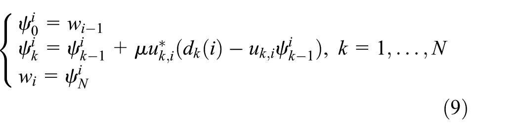
An incremental gradient solution is proposed^9,10 and described below

$$\{\begin{array}{c}{\psi }_0^i=w_{i-1}\hfill \\ \multicolumn{1}{c}{{\psi }_k^i={\psi }_{k-1}^i-\mu {[\nabla f_k({\psi }_{k-1}^i)]}^{*},k=1,\dots ,N}\\ \multicolumn{1}{c}{w_i={\psi }_N^i}\end{array}$$

(6)

The method (6) is referred as incremental LMS algorithm that is the nonlinear version of the LMS algorithm. Note that the important difference between (5) and (6) is that the gradients are evaluated at the different vectors w_i − 1 and ${\psi }_{k-1}^i$ , respectively.

By using an instantaneous approximations of the LMS type as follows

$$R_{u,k}\approx u_{k,i}^{*}{u}_{k,i},R_{\mathrm{du},k}\approx d_k(i)u_{k,i}^{*}$$

(7)

and substituting equation (7) into equations (5) and (6), the network-based steepest-descent and incremental LMS algorithms for distributed estimation can be implemented into practice in the following forms

$$\{\begin{array}{c}{\psi }_0^i=w_{i-1}\hfill \\ \multicolumn{1}{c}{{\psi }_k^i={\psi }_{k-1}^i+\mu u_{k,i}^{*}(d_k(i)-u_{k,i}{w}_{i-1}),k=1,\dots ,N}\\ \multicolumn{1}{c}{w_i={\psi }_N^i}\end{array}$$

(8)

and

$$\{\begin{array}{c}{\psi }_0^i=w_{i-1}\hfill \\ \multicolumn{1}{c}{{\psi }_k^i={\psi }_{k-1}^i+\mu u_{k,i}^{*}(d_k(i)-u_{k,i}{\psi }_{k-1}^i),k=1,\dots ,N}\\ \multicolumn{1}{c}{w_i={\psi }_N^i}\end{array}$$

(9)

After N sub-iterations, equation (8) is equivalent to the following form

$$w_i=w_{i-1}+\mu \sum _{k=1}^N{u}_{k,i}^{*}(d_k(i)-u_{k,i}{w}_{i-1})$$

Therefore, equation (8) can be called network-based steepest-descent algorithm, which is a hybrid of centralized steepest descent and distributed network implementation.

It can be seen from Figure 1 that algorithm (9) results in a fully distributed solution, which is more suitable for sensor networks with general applications. That is, each node k at the cycle path does not require the global information represented by w_i − 1. Instead, only local available information ${\psi }_{k-1}^i$ from its immediate neighbor is used to evaluate $\nabla f_k$ , thus reducing the additional resource consumption on communication. Moreover, we can see that the spatial diversity is fully exploited in equation (9) because each node accesses to the updated estimate ${\psi }_{k-1}^i$ and experiences the variation from the entire network.

Derivation of improved incremental LMS algorithm

Motivation

Despite the advantages noted above, we need to evaluate steepest-descent and incremental LMS algorithms in terms of performance. Analysis in this subsection will be presented on the basis of three important indicators including the impact of step size on convergence rate, steady-state convergence behavior, and oscillation.

Convergence rate

To simplify the analysis, we assume that each node on the cycle path has similar statistical distribution for input data, that is, R_u,k = R_u > 0 and R_du,k = R_du for k = 1,…,N. This assumption is valid when {u_k,i} arise from a single source with independent Gaussian distribution and commonly adopted to make tractable reasoning in Cattivelli and Sayed ¹⁰ and Khalili et al. ²⁹ And we introduce the eigendecomposition R_u = UΛU^*, where U is unitary and Λ is a diagonal matrix with the eigenvalues {λ₁,…,λ_M} of R_u.

Based on above assumption and optimization theory,^9–11w^o is the solution of the following equation

$$R_{\mathrm{du}}=R_u{w}^o$$

(10)

Substituting equation (10) into equation (6), we rewrite equation (6) as

$${\psi }_k^i={\psi }_{k-1}^i+\mu R_u(w^o-{\psi }_{k-1}^i)$$

(11)

By defining the weight error vector at node k as follows

$${\tilde{\psi }}_k^i\stackrel{\Delta }{=}{w}^o-{\psi }_k^i$$

(12)

and subtracting both sides from w^o for equation (11), we get

$${\tilde{\psi }}_k^i=(I-\mu R_u){\tilde{\psi }}_{k-1}^i$$

(13)

After N sub-iterations consisting of the cycle over the entire network starting from the vector ${\tilde{\psi }}_0^i$ , we have

$${\tilde{\psi }}_N^i=(I-\mu R_u{)}^N{\tilde{\psi }}_0^i$$

(14)

Similarly, using the following definition

$${\tilde{w}}^i\stackrel{\Delta }{=}{w}^o-w^i$$

(15)

Equation (14) can be rewritten as

$${\tilde{w}}^i=(I-\mu R_u{)}^N{\tilde{w}}^{i-1}$$

(16)

By substituting the eigendecomposition R_u = UΛU^* into equation (16), we get

$${\overline{w}}^i=(I-\mu \Lambda {)}^N{\overline{w}}^{i-1}$$

(17)

where ${\overline{w}}^i\stackrel{\Delta }{=}{U}^{*}{\tilde{w}}^i$ .

However, by rewriting equation (5) in the form

$${\psi }_k^i={\psi }_{k-1}^i+\mu R_u(w^o-w^i)$$

(18)

we have

$${\tilde{\psi }}_k^i={\tilde{\psi }}_{k-1}^i-\mu R_u{\tilde{w}}^{i-1}$$

(19)

After N sub-iterations

$${\tilde{\psi }}_N^i={\tilde{\psi }}_0^i-\mu N{R}_u{\tilde{w}}^{i-1}$$

(20)

equivalently

$${\tilde{w}}^i=(I-\mu N{R}_u){\tilde{w}}^{i-1}$$

(21)

Consequently, a different result can be derived for the steepest-descent algorithm, that is

$${\overline{w}}^i=(I-\mu N\Lambda ){\overline{w}}^{i-1}$$

(22)

Observing equations (17) and (22), there is a very different degree of descent or convergence rate for two algorithms during every iteration. To get a better look at them, taking the Euclidean norm of both sides of equations (17) and (22), we get

$$\Vert {\overline{w}}^i{\Vert }^2=({\overline{w}}^{i-1}{)}^{*}(I-\mu \Lambda {)}^{2N}{\overline{w}}^{i-1}$$

(23)

and

$$\Vert {\overline{w}}^i{\Vert }^2=({\overline{w}}^{i-1}{)}^{*}(I-\mu N\Lambda {)}^2{\overline{w}}^{i-1}$$

(24)

Specifically, considering λ_i = λ _j  = θ > 0 for 1 ≤ i ≠ j ≤ M, where θ is a real positive constant, we obtain

$$\Vert {\overline{w}}^i{\Vert }^2=(1-\mu \theta {)}^{2N}\Vert {\overline{w}}^{i-1}{\Vert }^2$$

(25)

and

$$\Vert {\overline{w}}^i{\Vert }^2=(1-\mu N\theta {)}^2\Vert {\overline{w}}^{i-1}{\Vert }^2$$

(26)

Based on equations (25) and (26), we define the convergence rate of incremental LMS algorithm

$$r_{\mathrm{inc}}=1-(1-\mu \theta {)}^{2N}$$

(27)

and convergence rate of steepest-descent algorithm

$$r_{\mathrm{steep}}=1-(1-\mu N\theta {)}^2$$

(28)

In order to compare the convergence rates of equations (27) and (28) against different step size μ, a numerical simulation is implemented with N = 20 and θ = 1. Figure 2 shows the simulation results when the step size μ varies between 0 to 0.1. We can make the following remark based on the observations in Figure 2.

Figure 2.

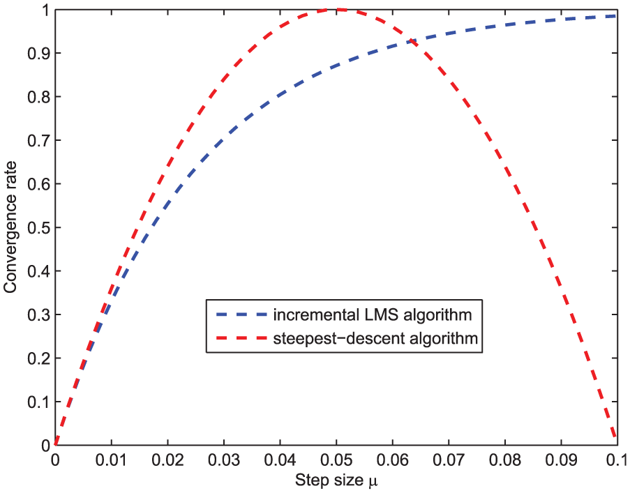
Convergence rate for algorithms (8) and (9).

Remark 1. The incremental LMS algorithm (9) has a faster rate of convergence than the steepest-descent algorithm (8) for fixed larger step size.

As a matter of fact, the known research results on gradient-like incremental methods show that step size is set to be large due to large system error in the early stage of algorithms, while the step size will be chosen as a smaller value as the algorithms converge to a state. Given the facts, some variable step-size LMS algorithms for distributed estimation have been proposed in Lee et al. ³⁵ and Saeed et al., ³⁶ where the advantages of the diminishing step sizes are confirmed theoretically and experimentally. From Remark 1, we can know that the incremental LMS algorithm is preferred to run in the early stage when a diminishing step-size method is adopted.

Steady-state convergence behavior

Based on the algorithm (9), the weight update on each node k is rewritten as

$$\begin{array}{c}{\psi }_1^i=w_{i-1}+\mu u_{1,i}^{*}(d_1(i)-u_{1,i}{\psi }_0^i)\hfill \\ \multicolumn{1}{c}{{\psi }_2^i=w_{i-1}+\mu u_{1,i}^{*}(d_1(i)-u_{1,i}{\psi }_0^i)+}\\ \multicolumn{1}{c}{\mu u_{2,i}^{*}(d_2(i)-u_{2,i}{\psi }_1^i)}\\ \multicolumn{1}{c}{⋮}\\ \multicolumn{1}{c}{{\psi }_{k-1}^i=w_{i-1}+\mu \sum _{t=1}^{k-1}[u_{t,i}^{*}(d_t(i)-u_{t,i}{\psi }_{t-1}^i)]}\\ \multicolumn{1}{c}{⋮}\\ \multicolumn{1}{c}{{\psi }_N^i=w_{i-1}+\mu \sum _{t=1}^N[u_{t,i}^{*}(d_t(i)-u_{t,i}{\psi }_{t-1}^i)]}\end{array}$$

(29)

Substituting ${\psi }_{k-1}^i$ in equation (29) into the second term on the right-hand side of (9), we obtain

$$\begin{array}{c}{\psi }_k^i={\psi }_{k-1}^i+\mu u_{k,i}^{*}(d_k(i)-u_{k,i}{w}_{i-1})\hfill \\ \multicolumn{1}{c}{-{\mu }^2{u}_{k,i}^{*}{u}_{k,i}\sum _{t=1}^{k-1}[u_{t,i}^{*}(d_t(i)-u_{t,i}{\psi }_{t-1}^i)]}\end{array}$$

(30)

Consider that diminishing step sizes are used in algorithms (8) and (9), in steady state (i.e. i→∞), it is known that the step size μ → 0 as ${\psi }_k^{\infty }$ converges to w^o. Thus, recursion (30) can be approximated by

$${\psi }_k^i={\psi }_{k-1}^i+\mu u_{k,i}^{*}(d_k(i)-u_{k,i}{w}_{i-1})$$

(31)

which is identical with equation (8).

Remark 2. In steady state, the incremental LMS algorithm (9) and the steepest-descent algorithm (8) tend to same convergence behavior when the diminishing step-size strategy is adopted.

Steady-state oscillation

The oscillation that occurs in steady-state (normal in the form of ripples) is very critical because it indicates the stability of the system and the accuracy of the algorithm. In general, the initial convergence rates of algorithms (8) and (9) are heavily dependent on a reasonable large step size as shown in Figure 2. After steady state is reached, the system is required for small amplitude oscillations that typically exist in gradient-based incremental techniques. In other words, the MSD between two successive iterations is expected to show less change.

Based on equations (25) and (26), we define the ratios

$${\rho }_{\mathrm{inc}}=1-r_{\mathrm{inc}}=(1-\mu \theta {)}^{2N}$$

(32)

and

$${\rho }_{\mathrm{steep}}=1-r_{\mathrm{steep}}=(1-\mu N\theta {)}^2$$

(33)

to depict the oscillations for the incremental LMS algorithm (9) and the steepest-descent algorithm (8), respectively. Consider the steady state where μ → 0 as the system error maintains at a stable and lower level, Figure 3 shows the numerical results following the same setting in Figure 2.

Figure 3.

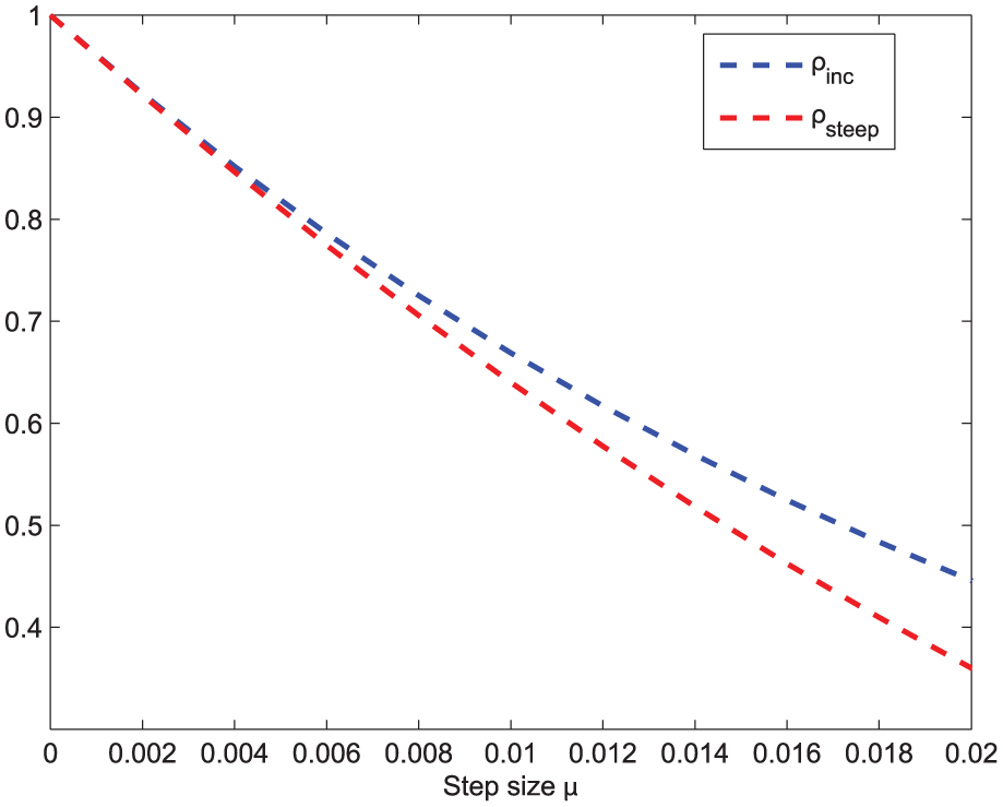
Illustration of steady-state oscillation for algorithms (8) and (9).

One can see from Figure 3 that the oscillation of the steepest-descent algorithm is smaller than the incremental LMS algorithm in the case of small step size. Although the difference between them is not so obvious, it has a big impact on stability and is magnified when the small system error is used as a comparison.

Consequently, we obtain the following remark:

Remark 3. In steady state, the steepest-descent algorithm (8) shows a smaller oscillation than the incremental LMS algorithm (9) when the diminishing step-size strategy is adopted.

Taking Remarks 1–3 into consideration, our main objective is to design a distributed estimation algorithm that combines the faster initial convergence rate of incremental LMS with smaller steady-state oscillation of steepest descent. Such that the designed method starts out as the incremental LMS, but gradually, it becomes more and more steepest descent, and in steady state, it approaches the steepest-descent method. Furthermore, this improved algorithm needs to use the variable step-size techniques with low computation complexity due to the energy limit of WSN.

Proposed incremental distributed LMS algorithm

Based on the motivations above, we propose an improved incremental LMS distributed algorithm with the combination of the merits of two strategies (8) and (9). That is,

The derivation of the proposed algorithm is straightforward but reasonable and performance efficient. Specifically, we employ two i-dependent parameters μ_i and σ_i, where μ_i plays a role of variable step size and σ_i adjusts the transformation speed from incremental LMS to gradient steepest. It is important to note several scalars that are used to obtain recursively μ_i and σ_i, such as μ_max is a constant that ensures that the MSE of the algorithm remains bounded, μ_min is chosen to ensure the minimum convergence speed in the fixed step-size case of LMS algorithm,^37,38δ > 0 is a small regularization parameter to avoid division by zero and adjust the diminishing rate of step size, and α > 1 and β > 0 are fixed scalars to ensure σ_i is increased as algorithm runs.

We see from algorithm 1 that in the special case where i = 1, we have μ_i ≈ μ_max and σ_i ≈ 0. At this time, algorithm 1 coincides with the incremental LMS algorithm (9). Following algorithm progresses, step size μ_i becomes smaller and σ_i becomes larger. Thus, algorithm becomes less incremental and more steep descent as i increases. From equation (29), we rewrite the updated weight estimate in algorithm 1

$${\psi }_k^i=w_{i-1}+{\mu }_i\frac{1}{1+{\sigma }_i}\sum _{t=1}^k{u}_{t,i}^{*}(d_t(i)-u_{t,i}{\psi }_{t-1}^i)$$

(34)

When i → ∞, we have that μ_i is a bounded value and σ_i → ∞ results in $\frac{1}{1+{\sigma }_i}\to 0$ . Consequently, we obtain the result of ${\psi }_k^i\to w_{i-1}$ . Thus, the differences between w_i and w_i − 1 is so small that there are few oscillations. By comparing (34) and (8), our algorithm approaches the steepest-descent algorithm with small steady-state oscillation.

Algorithm 1 The improved incremental distributed estimation algorithm.
Initialization: ${\psi }_0^i=w_{i-1}$ , ${\psi }_k^0=0$ , σ0 = 0
Iteration:
1: for every node k at iteration ido
2:  parameters: ${\mu }_i=\frac{{\mu }_{\max }}{\sqrt{i}+\delta }$
3:  σi = ασi − 1 + β
4:  ifμi < μminthen
5:   μi = μmin
6:  end if
7:  update:
8:   ${\psi }_k^i={\psi }_{k-1}^i+{\mu }_i\frac{1}{1+{\sigma }_i}{u}_{k,i}^{*}(d_k(i)-u_{k,i}{\psi }_{k-1}^i)$
9:  output: $w_i={\psi }_N^i$
10: end for

Therefore, the proposed algorithm meets the stated objectives, that is, diminishing step size with low computation complexity and transforming gradually from the incremental gradient to the steepest descent. Although various other variable step-size methods for LMS algorithm can be adopted,^29,35 their high computational requirement is a major obstacle for sensor networks with the objective of reducing energy consumption. For the network application without this restriction, the variable step-size algorithms with good adaptation performance is possible for further improvement. Here, we use only a simple variable step-size technique to match the transforming between the incremental gradient with the steepest descent. Moreover, compared with the incremental LMS, our algorithm has not any increase in communication cost. In other words, each node over network does not required any additional information from neighboring nodes to achieve the performance improvements.

The transforming strategy from the incremental gradient to the steepest descent can also be applied to the diffusion LMS mode, which consists of an incremental step and a diffusion step. According to the implementation order of two steps, CTA and ATC diffusion LMS algorithms are obtained. ¹¹ The changes should be embodied in the incremental step. Specifically, every node in the network performs an incremental update, during which the algorithm can easily be modified to get closer to the steepest-descent method using our strategy, such that the expected improvements can be achieved.

Mean stability analysis

In this subsection, the mean stability conditions will be derived to guarantee convergence in the mean of the weight estimate. To begin with, a data model on {d_k(i), u_k,i} is introduced as

$$d_k(i)=u_{k,i}{w}^o+v_k(i)$$

(35)

where v_k(i) is a zero-mean independent and identically distributed (i.i.d) sequence with variance ${\sigma }_{v,k}^2$ and independent of {d_l(j),u_l,j} for all l,j. Such data model is customary in distributed estimation methods^4,9,10,20,26 and will be applied to the target localization for sensor networks in the next section.

Subtracting w_o from both sides of the update equation in our algorithm, and using the data model (35) leads to

$${\tilde{\psi }}_k^i=[I-\frac{{\mu }_i}{1+{\sigma }_i}{u}_{k,i}^{*}{u}_{k,i}]{\tilde{\psi }}_{k-1}^i-\frac{{\mu }_i}{1+{\sigma }_i}{u}_{k,i}^{*}{v}_k(i)$$

(36)

By defining that ${\epsilon }_i\stackrel{\Delta }{=}\frac{{\mu }_i}{1+{\sigma }_i}$ , taking expectations of both sides and using the independence of v_k(i), we have

$$E[{\tilde{\psi }}_k^i]=[I-E({\epsilon }_i)R_{u,k}]E[{\tilde{\psi }}_{k-1}^i]$$

(37)

where an assumption is used for deriving equation (37), that is

Assumption 1: For algorithm 1, the step size ε_i is independent of input regressors u_k,i and weight error component ${\psi }_{k-1}^i$ .

Because μ_i is bounded and β is very small, ε_i will be close to its mean value. By writing

$$\begin{array}{c}E[{\epsilon }_i{u}_{k,i}^{*}{u}_{k,i}{\tilde{\psi }}_{k-1}^i]=E[{\epsilon }_i]E[u_{k,i}^{*}{u}_{k,i}{\tilde{\psi }}_{k-1}^i]\hfill \\ \multicolumn{1}{c}{+E[{\epsilon }_i-E({\epsilon }_i)]E[u_{k,i}^{*}{u}_{k,i}{\tilde{\psi }}_{k-1}^i]}\end{array}$$

(38)

we think that Assumption 1 holds asymptotically. And this assumption has been used widely and verified both theoretically and experimentally.^35,36,39

Iterating equation (37) and setting k = N, the weight-error vector on node N is updated in the form

$$E[{\tilde{\psi }}_N^i]=\{\underset{k=1}{\overset{N}{\Pi }}[I-E({\epsilon }_i)R_{u,k}]\}E[{\tilde{\psi }}_N^{i-1}]$$

(39)

or equivalently

$$E[{\tilde{w}}^i]={\displaystyle \prod _{k=1}^N[I-E(}{\epsilon }_i)R_{u,k}]E[{\tilde{w}}^{i-1}]$$

(40)

Equation (40) is stable or algorithm 1 is convergent in the mean if and only if

$$\underset{k=1}{\overset{N}{\Pi }}[I-E({\epsilon }_i)R_{u,k}]\to 0,\mathrm{as}i\to \infty$$

(41)

A sufficient and stronger condition for equation (41) to hold is obtained

$$E[{\epsilon }_i]<\frac{2}{{\lambda }_{\max }(R_{u,k})},1\le k\le N$$

(42)

where λ_max(R_u,k) denotes the maximum eigenvalue of R_u,k.

For practical usage, each node can set the parameters α and β to guarantee the convergence of algorithm based on the instantaneous approximations on R_u,k. Therefore, the mean stability condition (42) provides a guideline in choosing the appropriate parameters in our algorithm. The typical values of α and β that were found to work well in simulations are α = 1.00008 and β = 0.0006.

Application to target localization

To illustrate the effect of proposed algorithm, we consider this improved incremental distributed estimation applied to target localization, which is one of the basic technologies supported for many applications in WSNs, such as search, rescue, disaster relief, and target tracking. Target localization aims to estimate the position of static targets located in the sensing field of WSNs.

According to whether the measurements related to distance or angle between two nodes are needed, target localization can be classified as range-based and range-free. For range-based schemes, distance or angle is obtained by small amounts of the anchor or beacon nodes that are aware of their own positions (either via Global Positioning System (GPS) device or from a system administrator). The known measurement-based localization techniques include time-based methods (e.g. time of arrival (TOA) ⁴⁰ and time difference of arrival (TDOA) ⁴¹ ), received signal strength indicator (RSSI), ⁴² and angle of arrival (AOA). ⁴³ For range-free schemes, the acquisition of the position information of the target depends on the information about neighbor connectivity or hop-count in multi-hop WSNs instead of the measurements. ⁴⁴ Range-free method is cost-effective but low-precision, in contrast, range-based method aims to reach the general goal of high precision with a broader range of applications. In this article, we apply the proposed algorithm to the problem of target localization based on distance measurement in the two-dimensional (2D) scenario.

Following our previous notations, the actual location of the unknown target is denoted by the 2 × 1 column vector w^o = col{x^o, y^o}, which is estimated iteratively. Assume that the anchor nodes are organized in a directed cycle and know their precise position denoted by p_k = col{x^k, y^k}, where k indicates the anchor node. The actual distance between the anchor node k and the target is $r_k^o$ obtained by

$$r_k^o=\Vert w^o-p_k\Vert$$

(43)

where ‖·‖ denotes the Euclidean norm.

At iteration i, each anchor node k collects the noisy distance measurement $r_k^i$ denoted by

$$r_k^i=r_k^o+v_k(i)$$

(44)

where the noise v_k(i) is assumed to be zero-mean, and temporally white and spatially independent with variance ${\sigma }_{v,k}^2$ .

The unit direction vector $u_k^o$ pointing from the anchor node k toward the target is given by

$$u_k^o=\frac{{(w^o-p_k)}^T}{\Vert w^o-p_k\Vert }$$

(45)

where (·) ^T denotes the transpose of a vector.

At iteration i, each anchor node k also measures the noisy direction vector denoted by u_k,i, which is modeled by

$$u_{k,i}=u_k^o+a_k(i)u_k^{o\perp }+b_k(i)u_k^o$$

(46)

where $u_k^{o\perp }$ is a unit row vector that is perpendicular to $u_k^o$ , and a_k(i) and b_k(i) are the zero-mean spatially independent random noises, whose variances are assumed that

$${\sigma }_{a,k}^2=E|a_k(i){|}^2,{\sigma }_{b,k}^2=E|b_k(i){|}^2$$

(47)

As shown in Figure 4, the measured direction vector u_k,i is perturbed slightly along the directions of $u_k^{o\perp }$ and $u_k^o$ . We assume that the disturbance caused by the perturbation is small. Based on the knowledge of measuring direction through sensors, it is further assumed that the deviation along the parallel direction is small compared to the deviation along the perpendicular direction, as well as the distance noisy v_k(i), that is

$${\sigma }_{b,k}^2<<{\sigma }_{a,k}^2,{\sigma }_{b,k}^2<<{\sigma }_{v,k}^2$$

(48)

Figure 4.

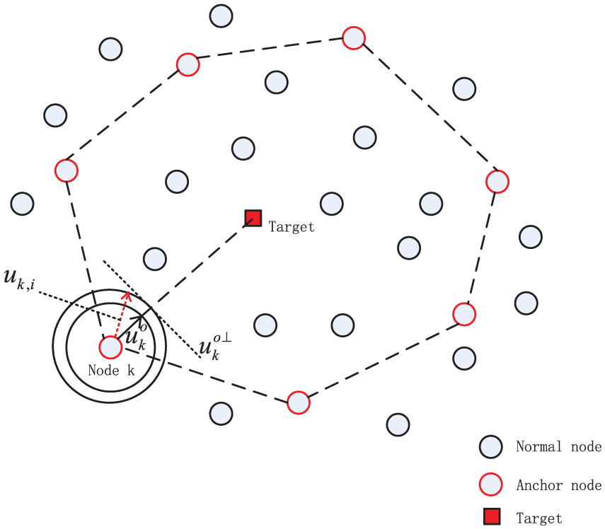
Illustration of target localization using incremental distributed estimation algorithm.

Combining equations (43), (44), and (45), we have the equation related to $r_k^i$

$$r_k^i=u_k^o(w^o-p_k)+v_k(i)$$

(49)

Substituting equation (46) into equation (49) yields

$$\begin{array}{c}{r}_k^i=u_{k,i}(w^o-p_k)-a_k(i)u_k^{o\perp }(w^o-p_k)\hfill \\ \multicolumn{1}{c}{-b_k(i)u_k^o(w^o-p_k)+v_k(i)}\\ \multicolumn{1}{c}{=u_{k,i}(w^o-p_k)-b_k(i)r_k^o+v_k(i)}\\ \multicolumn{1}{c}{\approx u_{k,i}(w^o-p_k)+v_k(i)}\end{array}$$

(50)

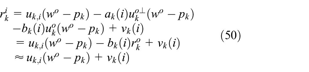
Rewriting equation (50) as follows

$$r_k^i+u_{k,i}{p}_k\approx u_{k,i}{w}^o+v_k(i)$$

(51)

We define that

$$d_k(i)\stackrel{\Delta }{=}{u}_{k,i}{w}^o+v_k(i)$$

(52)

which is consistent with equation (35) and obtained approximately through (51), in which the variables $r_k^i$ and u_k,i can be measured by anchor node k at time i.

Assuming that the target position vector estimated by node k at time i is also denoted by ${\psi }_k^i$ , the update equation is similar to that one in algorithm 1. The only difference is that d_k(i) is given by equation (52). Therefore, by measuring the distance $r_k^i$ and direction vector u_k,i with the same target, all anchor nodes can cooperatively obtain the estimate wⁱ until the error satisfies the measuring requirement.

It should be noted that for the target-tracking applications, an adaptive step-size mechanism instead of diminishing step size should be adopted. More specifically, by measuring the deviation on the distance $r_k^i$ and direction u_k,i between two contiguous periods, the algorithm should use the large step size to accelerate convergence and improve traceability once a sudden change on the target is detected, while the diminishing step size can be used in a relatively stable state to achieve the high accuracy.

Simulation results

In this section, we provide the computer simulation results for performance comparison of proposed algorithm and the incremental LMS algorithm. The key performance indicators such as convergence speed, steady-state error, and oscillation are shown on the basis of the transient network MSD, which is defined by

$$\mathrm{Transient}\mathrm{network}\mathrm{MSD}=E\Vert {\tilde{w}}^i{\Vert }^2=E\Vert {\tilde{\psi }}_N^i{\Vert }^2$$

(53)

Moreover, the application effect of proposed algorithm for the problem of target localization will be evaluated.

Performance comparison

In this simulation, we implement the performance comparison between the incremental LMS and our algorithm under the typical data condition.^10,26,27,29 The network topology consists of 20 nodes that are assumed to communicate in a way of Hamiltonian cycle. The regressor {u_k,i} on each node is independent Gaussian with random input power ${\sigma }_{u,k}^2\in (0,1]$ (Figure 5(a)) and the background noise is white and Gaussian with random power ${\sigma }_{v,k}^2\in (0,01]$ (Figure 5(b)). The corresponding signal-to-noise ratio (SNR) is shown in Figure 5(c). The estimated weight vector $w^o=\mathrm{col}\{1,1,\dots ,1\}/\sqrt{M}$ with the length M = 10 is unknown for evaluated algorithms but known for us due to the need to evaluate. Thus, the noisy measurement d_k(i) can be generated via equation (35). For the proposed algorithm, we set μ_max = 0.05, μ_min = 0.0001, α = 1.00008, and β = 0.0006.

Figure 5.

(a) Node power profile, (b) noise power profile, and (c) signal-to-noise ratio profile.

To get the better understanding of network behavior, the network MSD is plotted in decibels as a function of number of iterations. It is important to note that the performance difference between the incremental LMS and the steepest decent only can be observed after the results are averaged over a certain amount (i.e. 500), while the average result will greatly weaken the oscillating amplitude in steady state. Thus, we provide the MSD comparison results for one random experiment between incremental LMS algorithm with three different constant step sizes and proposed algorithm. The detailed performance advantages of the incremental LMS against the steepest decent can be found in related studies.^9,10 The role of constant step size is to show three advantages of proposed algorithm over conventional incremental LMS algorithm in convergence speed, steady-state error, and oscillation.

For convergence speed, first, we can see from Figure 6 that the incremental LMS algorithm with larger step size is faster than the ones with smaller step size. For steady-state error, the picture is reversed. However, our algorithm is effective for both quickening the initial convergence and reducing the steady-state error. However, we can also observe that the huge steady-state oscillation appears in the incremental LMS algorithm whether the step size is large or small. In Figure 6, we can clearly see that our algorithm shows no significant oscillation in steady state. As already analyzed, the reason is that our method has a very small differences between two successive estimated vectors as i → ∞. Based on the above, one can draw a conclusion that the proposed method outperforms the incremental LMS algorithm in three aforementioned performance indicators.

Figure 6.

MSD comparison between incremental LMS algorithm with three different step-sizes and proposed algorithm.

In order to illustrate individually the effect of transforming from the incremental gradient to the steepest descent, the incremental LMS algorithm with same diminishing step size is compared with the proposed algorithm. In other words, equation (9) is rewritten as

$${\psi }_k^i={\psi }_{k-1}^i+\frac{{\mu }_{\max }}{\sqrt{i}+\delta }{u}_{k,i}^{*}(d_k(i)-u_{k,i}{\psi }_{k-1}^i)$$

(54)

Equation (54) is denoted by the traditional diminishing step-size incremental LMS algorithm without transforming from the incremental LMS to the steepest descent. From Figure 7, it is clear that the proposed algorithm has smaller steady-state error and oscillation, and similar convergence speed because it can be regarded as incremental LMS algorithm at the initial stage. From this simulation, we can see that the performance improvements of incremental LMS algorithm result from the combination of the proposed transforming strategy and diminishing step size.

Figure 7.

MSD comparison between incremental LMS algorithm with diminishing step size and proposed algorithm.

In conclusion, simulation results show that our algorithm outperforms the incremental LMS, both to constant step size and to diminishing step size. As pointed out by previous theoretical analysis, the reason is that our algorithm combines the merits of incremental LMS and steepest-descent algorithms to achieve the goal of faster initial convergence rate and smaller steady-state oscillation.

Target localization

For the proposed algorithm used for target localization, we adopt a common node deployment condition similar to Chen et al. ⁴⁵ and Savic and Zazo ⁴⁶ and assume that the sensor network consists of N = 50 nodes that are randomly distributed on a square area of 10m × 10m. As shown in Figure 8, the position of the target located in the area is random and unknown. Eight anchor nodes that know their positions exactly are used to measure the distance and direction vector with target. The distance noise v_k(i) and direction vector noise a_k(i) are zero-mean spatially independent with variance ${\sigma }_{v,k}^2\in (0,01]$ and ${\sigma }_{a,k}^2\in (0,001]$ , respectively. Each anchor node runs equation (51) at every iteration to obtain {d_k(i),u_k,i}, such that the position of the target is estimated successfully as algorithm 1 runs. The same parameter settings as previous subsection are used.

Figure 8.

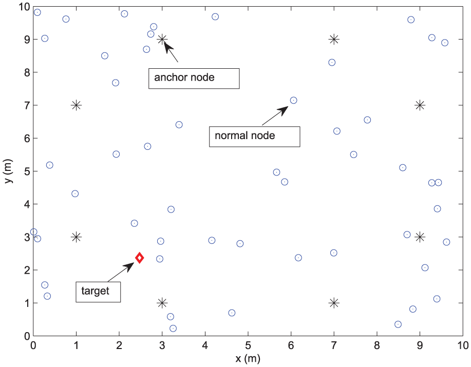
Illustration of the simulated sensor network used for target localization.

Figure 9 shows the estimation error changing curve of incremental LMS algorithm with a constant step size μ = 0.002 and diminishing step size, and proposed algorithm for one random selected experiment, where the error is defined as the Euclidean distance between actual position and estimated position. Similar to equation (54), the incremental LMS algorithm with diminishing step size is also applied to the localization example and the results are given in Figure 10. Figure 10(b) is a larger version of Figure 10(a) for 100 iterations from time 300 to 400. To summarize the above simulation results, the improvements achieved by the proposed estimation algorithm are obvious from the aspects of convergence speed, steady-state error, and oscillation, all of which are critical for real applications.

Figure 9.

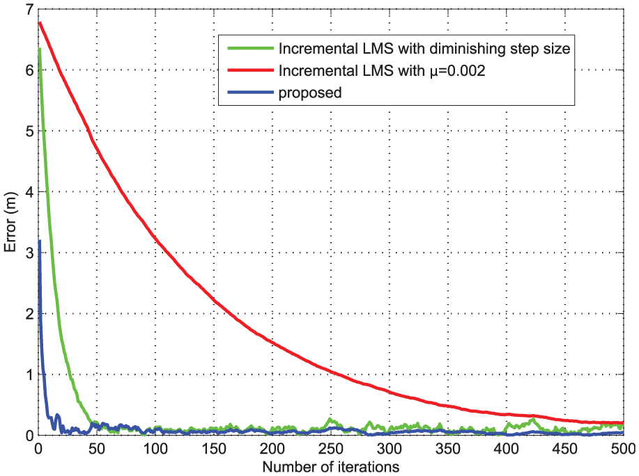
Estimation error change of incremental LMS algorithm and proposed algorithm.

Figure 10.

(a) Estimation error change for 500 iterations and (b) estimation error change for 100 iterations from 300 to 400.

We can also see from Figure 10(b) that the estimation accuracy is sufficient to meet the application requirement. It should be pointed out, however, one difficulty with our method is the large number of iterations, which will lead to high communication and computation load. An effective way to solve the problem is to gather the preliminary information of unknown target during the initialization phase of algorithm. As described in our algorithm, the unknown vector is estimated with a starting value of 0. The number of iterations will be greatly reduced when the rough initial status about the target is available. Consider the case of tracking mobile target with a slow movement, the next actual location of the target is very close to the present estimated location, thereby saving a lot of time used for convergence.

Conclusion

In this article, we compared the incremental LMS and the steepest decent for the problem of distributed estimation in the case of diminishing step size. The main goal is to achieve the performance improvements on convergence speed, steady-state error, and oscillation. A new incremental distributed estimation algorithm is proposed for WSNs with the application of target localization. The mean stability condition of the proposed algorithm is derived for the guideline in practice. Simulation results verified the improvements and application effect for target localization in WSNs. In future study, the proposed algorithm will be extended for such cases of the noisy link and missing data over WSNs.