Sage Journals: Discover world-class research

Abstract

We present challenges faced deploying a solar-powered wireless sensor network base station and nodes, at a remote oyster farm. It involved installing the base station system and a data server at the shore of a shallow bay, where there is no electrical power available. To solve the problem, we set up a photovoltaic array with an energy monitoring node, from which performance metrics were recorded and plotted. At the water, we deployed two wireless sensor nodes on a raft, a kilometre away from the base station. One node was configured for sea water pH and water temperature (T_w) measurements. The other node was configured for salinity and T_w measurements. Furthermore, both nodes measured air temperature and relative humidity, for a more complete characterization. At the salinity node, temperature and relative humidity knowledge was crucial to determine a gain factor for doing a trial of a transmission power control scheme, using a novel temperature and relative humidity algorithm. To enable a fair comparison, the pH nodes transmitter was configured with a fixed power level. The nodes performances were measured locally at the base station, recording metrics such as received signal strength indicator and packet received rates.

Keywords

Wireless sensor networks transmission power control renewable energy ubiquitous computing remote monitoring

Introduction

Marine habitat monitoring has always been a challenge due to the inhospitable nature of the surroundings. Electronic systems and sensors have to be carefully encased and made seaworthy. When sensors are deployed to withstand the environment, mechanical and electrical stress can have an undesired impact on their response and behaviour.^1,2 Another common issue is the non-availability of electrical power sources; for which nowadays this is resolved deploying solar renewable energy. Solar panel use is now becoming a standard solution and wind turbines as a second choice.^3–5 Obviously, for any solution, the surroundings are key for choosing which is more appropriate. Although marine life is not considered as interfering factors in the conventional systems operations, often they are the main reason of renewable power systems failure due to animal tampering, such as birds ‘fowling up’ solar panels.^6,7 Smart energy systems are now possible and can be built with lower cost materials, and to make them versatile, microcontrollers can now be easily included to monitor and opportunely worn of unwanted power variations.

Regarding communication issues, there is the concern of the type of channel that represents transmitting over sea water, where fading losses may be experienced due to electromagnetic (EM) vapour absorption.^8,9 Other fading sources include radiofrequency (RF) reflexions on the water surface, which especially hampers this type of EM propagation. At the destination, the received signal strength may fall below the radio sensitivity and considered noise, and if demodulated, considerable bit errors may occur affecting the overall packet received rate (PRR).

Early environmental data acquisition had the limitation that timely information was impossible because data were registered locally on paper. It entailed having to go for the information which could take days, weeks or even months to obtain. Nowadays, data acquisition has progressed significantly, and sensor systems now have digital capabilities that can communicate through network connections, so they can deliver data immediately, after sensing the observed medium or variable.^10,11 Nevertheless, dense sensor network deployments, in harsh environments, is a complex task (or group of tasks) that involve sophisticated electronic systems. First of all, power supply issues are a primary concern due to the lack of energy outlets in a natural or aquatic environment.^12,13 Some systems and operations have high energy requirements that can’t easily be met. Battery operation has issues that have to be addressed, and solutions are found due to well-outlined deployment plans. Some do it yourself (DIY) environmental monitoring green energy solutions are readily available, but there is no guarantee that they can be applied in a dynamic and harsh environment. Hence, electronic sensing systems and communication links have to be robust enough to withstand extreme conditions, including wild animal interference, such as rodent or bird activity near cables and solar panels.

On the other hand, for the kind of application scenario we present here, common variables measured by ocean wireless sensor network (WSN) deployments are temperature, pressure, depth, tide direction, pH, turbidity, flow rate, salinity and dissolved oxygen;¹⁴ other measured variables may even be for detecting pollutants such as heavy metals or radiation. For years, many long-distance sensor networks have used radio repeaters that deploy hierarchical sensor node architectures, which are still useful.^15,16 For a water monitoring system to succeed, it must be enclosed onboard a seaworthy floating buoy or raft. The basic problem is moisture, which represents the most difficult aspect to overcome. Another issue is the lack of an electrical power source, which today is dealt with using renewable energy generation. Figure 1 shows a conceptual model of a seaworthy vessel for lodging the electronics for sea monitoring.

Figure 1.

Components of a seaworthy monitoring sensor system.

In a remote application, such as this, solar energy harvesting and its corresponding battery powered system are required features to keep the electronics functioning. Likewise, a robust RF communication system is now essential to maintain monitoring operations. Regarding buoy position, some marine systems have GPS (Global Positioning System) receivers installed in case the floating device’s mooring line gets loose from its anchor. Regardless of the sophistication, as previously shown in Figure 1, an ocean monitoring system requires having one or more underwater sensors, at least it must be capable of measuring water temperature, and it all depends on which ocean variables are of interest.

Background and related work

This is a continued effort of a bigger project, and the contributions of this work are threefold: (1) reporting continued experiences of deploying real marine WSN nodes, in harsh conditions;¹⁷ (2) reporting results of the deployment of a performance monitored renewable energy system, which supplies power to the on-shore WSN autonomous base station (BS) system; and (3) corroborating reliable data delivery using our novel temperature and relative humidity transmission power control algorithm (or TRH-TPC), for environmental WSN communications.¹⁸ This aspect of our deployment focuses on a real long-range TRH-TPC trial run, which lasted several days; based on our algorithm, which we described, modelled, simulated and preliminary tested, this venture was reported in an earlier publication.¹⁹

Oyster farm end-to-end telemetry architecture

At Bahia Falsa, Baja California, Mexico, the main commercial activity is a growing aquaculture industry, mainly oyster farming, and now they are producing clams and other mollusks.²⁰ Bahía Falsa has fluctuating ocean tide schedules, where different water variables have extreme changes according to water level conditions.^21,22 In Figure 2, a composite satellite image is shown of the area where the BS was placed, and where both CLH-1 and CLH-2 nodes communicated directly with the BS at a 1200 m distance. For oyster farm operations in the region, the concern is having timely sea water quality measurements of variables such as temperature, pH and salinity. Interest is focused on sensing conditions near their live oyster underwater storage area, located offshore a kilometre and a half away from their dock and main office. The main water variable is temperature, which the oyster producers sometimes measure manually.²³ As water temperature increases sharply and stays warm (above 20°C), the toxic blue-green algae may bloom and may promote unsanitary stagnation conditions, depleting the water’s dissolved oxygen content vital for the oysters’ survival.^24,25 Aquaculture farm oysters grow within metal containers, which the growers can extract from the bay if water conditions are questionable.

Figure 2.

Bahia Falsa base station and node placement.

WSN upper-tier implementation

Figure 3 shows the proposed hierarchical WSN which we previously tested in a very limited two-hop messaging operation,¹⁷ with no transmission power control what so ever. It is hierarchical because it is made up of a lower tier and an upper tier. At the lower tier, clusters are formed by 2.4 GHz end-point (EP) nodes that gather sensor data and send it to their cluster-head (CLH) node. At the 900 MHz upper tier, CLH nodes take their sensor readings and create an application message; this message also includes their buffered cluster EP data (received earlier) and other CLH performance values. Then, using a simple time synchronization scheme, each CLH node transmits a structured sensor data message to its BS. Here, we prepared a trial run of the upper tier with two 900 MHz cluster-heads, with water quality sensors. The novelty in what we present here, with these CLH nodes, is that they operated for several days in real long-range conditions, with the aim of using their results to corroborate previous CLH tests that only used RF attenuators to emulate distance in very limited outdoor experiments.¹⁸

Figure 3.

Dual-frequency hierarchical WSN.

It is worth noting that complete CLH wireless nodes are composed of three printed circuit board layers, in a printed circuit board (PCB) stack configuration. The bottom layer of the hardware stack is a common Arduino Mega controller board.²⁶ Using the same footprint, we developed a 900 MHz and 2.4 GHz transceiver interface shield, which is the second stack layer that goes on top of the Arduino Mega. And as the third layer, we previously developed a PCB shield specially made for our application sensor connections, which stacks on top of the radio shield.

WSN application messages

At the application layer, CLH wireless nodes and BS system communicate with each other using a modified JSON for WSN message exchanges, and we call it ‘Light’ JSON or LJSON.^27,28 A simple generalized message is shown in Figure 4, where it has a heather that starts with the ID of the cluster-head that sends the high tier light-JSON message.

Figure 4.

A simple LJSON message.

In this example (Figure 4), the C symbol is the nodes ID, C:1, T is the UNIX time-stamp, T:1455843248, the parameter An:4 indicates four sensor values acquired by the cluster-head, Av is the sensor value array with four elements and r is the received signal strength indicator (RSSI) value of the last BS message received by CLH 1. Afterwards, the symbol e indicates an array of EP object messages, i is the EP identifier and the other symbols are equivalent to the CLH message tag descriptions. Other data can be embedded in the message hierarchy. In this case, the first sensor value in the array is an air temperature times ten, followed by water temperature times ten, then air relative humidity percentage, and ends with ten times the pH value measured by CLH-1. We opted to send some values scaled up (10 times) to avoid sending the floating point character; at the server, these values are scaled back to have decimal point values dividing them by 10. Other parameters and measurements can be included in the message in the form of tag:value pairs. At the BS, decoding algorithms extract pertinent information from the incoming LJSON messages (such as the BS RSSI), then a JSON encoding algorithm adds other information (such as the CLH RSSI measured by the BS) along with the received data, and sends it to the data server. If EP information were to be received by a CLH system, then a more complex LJSON message would be created, with added parameters such as EP time stamps.

BS gateway and co-state operations

In our prior deployment, the RCM4300 controller module²⁹ was selected and used as the core of our BS system, it has several serial ports, EEPROM and a permanent real-time clock system (coin battery powered). We attached the so-called AC4490 900 gMHz digital transceiver^30,31 to one of the RCM serial ports. It is worth mentioning that an important feature of the RCM4300, which stood out during initial technology selection, is that it has an Ethernet interface chipset. This enables the RCM4300 to have IP network connections, which is also supported by a complete license free TCP/IP software library. In light of these capabilities, this BS is multifunctional because it serves as the sink node controller of the WSN and as an IP gateway through its Ethernet interface.

Regarding software development, the RCM4300 is oriented to run in a state machine manner, using the Rabbit Corp. Dynamic C (now owned by Digi Inc.).³² Where you can implement their unique software model paradigm they call ‘co-state’ operation. In a co-state paradigm, code is segmented in pieces that runs sequentially with the rest of the code, but the programme pointer may jump into or out of them, if it encounters wait states or depending on a particular flag that may change due to an external hardware or serial event, similar to an interrupt but with state machine approach. The operational BS models are shown in Figures 5 and 6.

Figure 5.

Time request on BS start up.

Figure 6.

Model of normal CLH to BS and BS to Data Server data acquisition operations.

When the WSN BS starts its operation, it requests an updated Time Stamp from the Data Server, which could be Internet hosted, or at a Local Host. This process has a time-out interrupt, in case the TCP/IP connection can’t be established; and for which a local default Time Stamp is used, which may be running on a solid-state real-time clock, even if the processor and main programme is started or reset.

During normal operations, the BS sends a time stamped beacon message every 60 s through its AC4490 sink radio. Out on the field, the CLH wireless sensor nodes synchronize their clocks with the BS beacon message, this puts in sync their sampling and transmitting periods. Furthermore, this beacon can easily be configured for different sampling rates, depending on the application. Our beacon approach is a simple and convenient way to synchronize a basic time division multiple access (TDMA) scheme, in which the cluster-heads send their sampled data according to their numerical assignment. For instance, with the default 60 s beacon, CLH-1 sends its data 1 s after it receives the BS beacon (time that is synchronized to its local time clock); likewise, if there is a CLH-2, then it sends its data 2 s after the beacon (on second after CLH-1). In the same way, a third cluster-head, CLH-3, will send its data 3 s after de beacon, and so on. With these default numbers, this TDMA scheme can have up to 59 cluster-heads transmitting data frames without collisions.

Figure 7 shows the cluster-head systems normal operations, besides doing their local sensor sampling tasks, they also may receive data from smaller EP systems. Afterwards, the CLHs create a composed local and EP data messages, which are subsequently sent to the sink node connected to the BS system.

Figure 7.

Normal CLH operations.

TRH transmission power control

Part of the problem of sea monitoring is that radio communications may be hampered by humid conditions, which causes EM energy absorption and fading. A typical solution is to transmit at a very high power level that is usually determined considering the worst-case scenario. On the contrary, when channel conditions are such that fading is not an issue, transmitting at higher levels than needed obviously wastes valuable electrical power. Another alternative is to deploy some kind of transmission power control so as to optimize power consumption during RF transmissions.

Transmission power control is useful where radio communication may encounter frequent fading, or when wireless node mobility is an important issue.³³ Here, we implemented a novel temperature and relative humidity gain factor Δ_N, which is based on equation (1) and is represented by equation (2). We previously published this approach with an extended analysis of its behaviour and performance¹⁹ and called it TRH-TPC because it uses temperature and relative humidity knowledge for controlling a radio transmitter’s power

\nabla (t) = \frac{T (t) R H (t)}{T_{m a x} R H_{m a x}}; 0 < \nabla (t) \leq 1

(1)

Δ_{N} = 1 - e^{- α_{0} (1 - \nabla (t))}

(2)

Equation (1) has no physical representation; it is a proposed normalized gradient only, where T(t) is the measured air temperature and RH(t) is its relative humidity. While in equation (2), α₀ is a dampening coefficient, which can take different values that affect the resulting magnitude for power compensation. The α₀ coefficient is intended to avoid transmitter power saturation when both T and RH are high. In this implementation, we used the updated TRH-TPC model and algorithm that we published and completely explained, which requires two set points to operate: a maximum RSSI level and minimum RSSI. With those RSSI reference values, TRH-TPC power compensation does the following:

If RSSI(k − 1) < RSSImin:

PL(k+1)=PL(k)+DN(RSSImin − RSSI(k − 1))

Else if (RSSI(k − 1)<RSSImax:

PL(k+1)=PL(k) − DN(RSSImax+RSSI(k − 1))

where RSSI(k − 1): last reassured RSSI; RSSImin: minimum RSSI threshold; RSSImax: maximum RSSI threshold; DN: TRH-TPC compensation function; PL(k): current Tx power level; and PL(k+1): next Tx power level.

Experimental setup

The three main issues that are dealt and resolved in this work are (1) the solar-powered BS setup and monitoring, (2) the challenges of implementing electronic wireless water quality instrumentation on a sea water surface on board an experimental raft (Figure 2) and (3) overcoming wireless channel fading radiating over sea water using 900–915 MHz frequency hopping radios, and where a TPC approach is put to the test. But first the experimental setup is explained, starting with the WSN components, such as the solar-powered auto-sustainable WSN BS, then we describe the proposed long-range WSN. Afterwards, the preliminary instrumentation results are shown and discussed, and finally we present a discussion about the TRH-TPC algorithm results versus fixed Tx power performance.

Auto-sustainable WSN BS

At the shore of Bahia Falsa, there are no electrical outlets available; to solve the problem, we used solar panels, re-chargeable batteries and a DC to AC inverter to power an on-site data server. For performance monitoring, we included in our design a wireless DC to AC current monitoring node that sends pertinent power generating data to the BS.

The entire BS setup is illustrated in Figure 8, and it includes the wireless current monitoring system. And in Figure 9, the actual deployment is shown, where the BS was put in a sealed enclosure, setup on the roof of the oyster farm facilities. The wireless AC/DC power monitoring node establishes radio communications with the WSN BS, the difference with other sensor nodes is in the types of messages that are exchanged. The measured metrics are (1) DC current, (2) AC RMS current and (3) battery recharge cycles.

Figure 8.

Solar power subsystem with wireless monitoring.

Figure 9.

Actual BS and solar-powered system deployment on the roof of the Oyster farm offices at the shore of Bahia Falsa.

Deploying water quality monitoring on a seaworthy floating vessel

There are many seaworthy solutions for water monitoring that use floating buoys; the drawback of using buoys in a shallow bay is that they have a long vertical axis (with a counter weight) that may hit the bay floor during low tide. A more practical solution is to use a raft, with low tide posts that prevent haul damage, while keeping a horizontal floor orientation. In Figure 10, we show the raft we used for these trials. Pelicans, other sea birds and even sea mammals, such as seals, sometimes use it as a rest area while fishing. We put two CLH systems on opposing sides of the raft. The first system was CLH-1 node, installed inside the raft, next to an opening through which we put a temperature and a pH sensor in the water, as shown in Figure 11.

Figure 10.

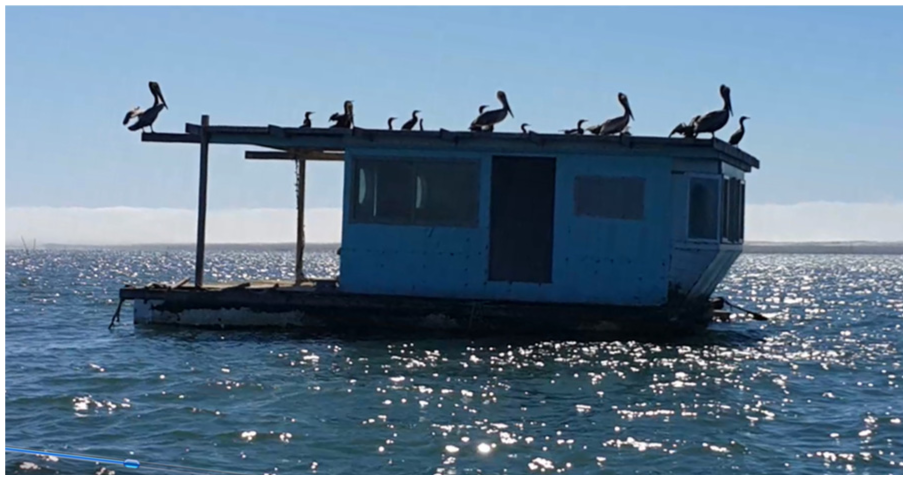
Oyster farm experimentation raft at the central canal of Bahia Falsa.

Figure 11.

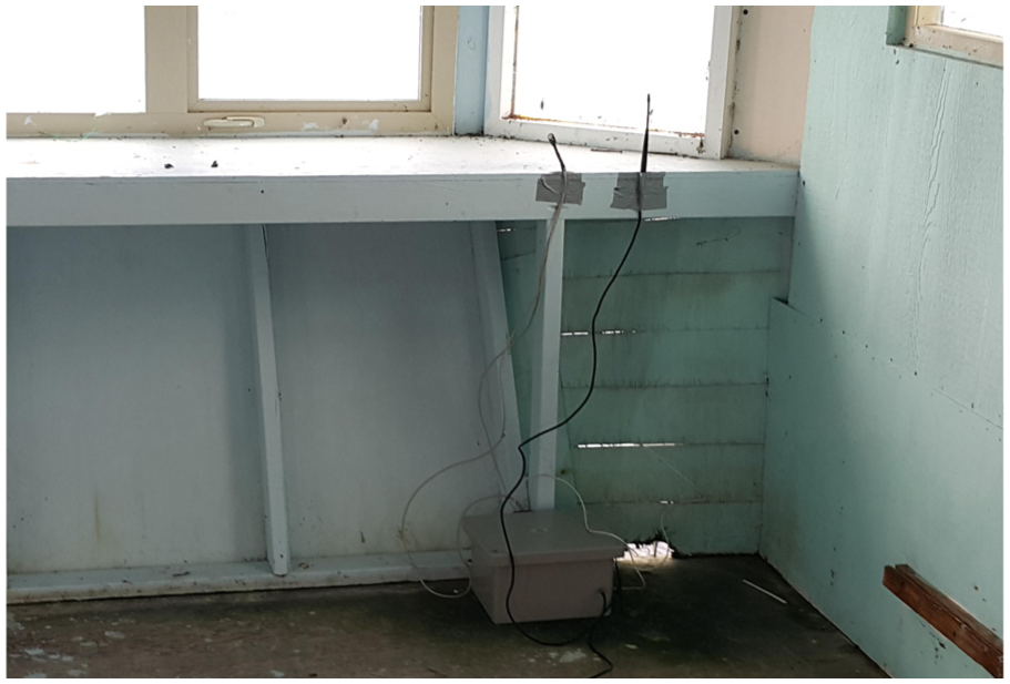
CLH-1 with temperature and pH sensors in the water, installed inside the raft.

Afterwards, we put CLH-2 outside on the rafts deck, with the salinity sensor hanging on the side submerged in the water, as shown in Figure 12. It is worth mentioning that, a week later after the setup, when we went back we found that both CLH nodes solar panels were covered with seabird guano, which is shown in Figure 13.

Figure 12.

CLH-2 with submerged water temperature and salinity sensors set up on the rafts deck.

Figure 13.

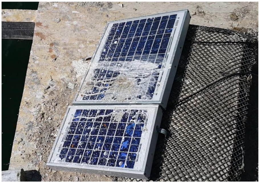
CLH-1 solar panel (top of the picture) and CLH-2 solar panel (bottom of the picture) were partially covered in seabird guano.

pH and salinity probe and their interface with the wireless nodes

For our next-generation wireless nodes, as mentioned previously, our cluster-head nodes are made up of three PCB boards: the microcontroller board, the 900 MHz–2.4 GHz radio shield; as a third hardware layer we developed a sensor interface board, for analogue and digital three wired sensors (temperature and relative humidity); and a separate connection for two Atlas Scientific mini-circuit interface boards, with a three-pinout water quality probe connectors. We chose Atlas Scientific water instrumentation because of their simplicity, low cost and rapid deployment. In this particular case, we used Atlas Scientific pH boards and conductivity measuring technology. Our sensor shield PCB layout is shown in Figure 14.

Figure 14.

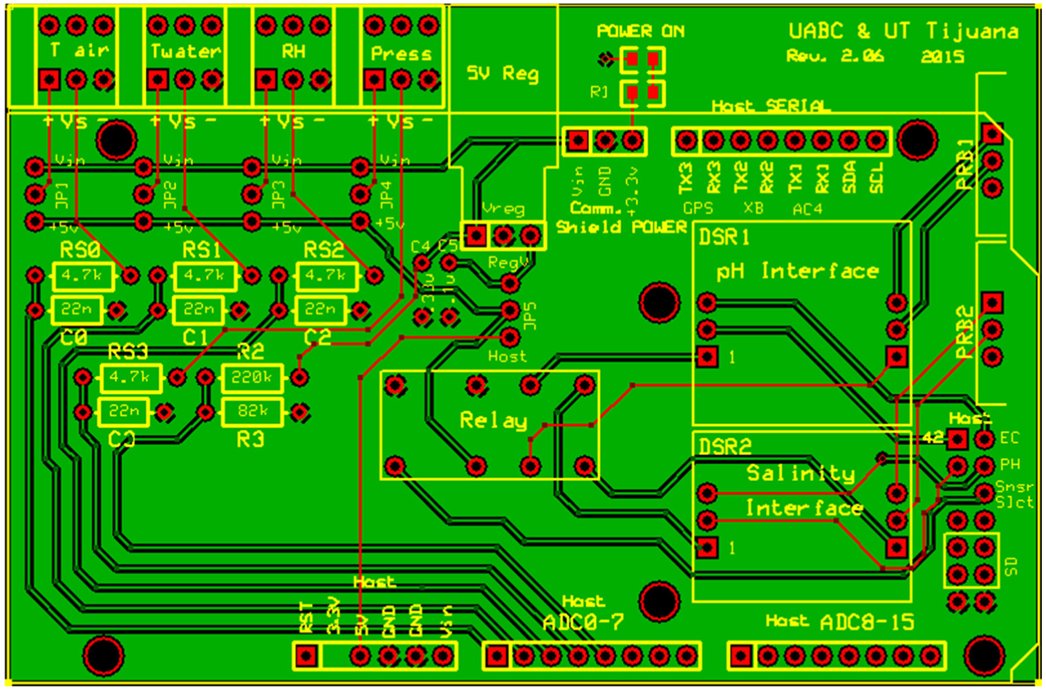
Sensor interface printed circuit board.

If multiple chemical probe readings are required on a single node, our sensor shield allows installing a medical instrumentation relay circuit, for software-driven probe switching. In this test, only one probe was attached at a time to any of the test nodes that were put on the water.

Combined results and comments

Here, we present results of water sensor readings, pertaining to the application variables for oyster farming, such as temperature, salinity and pH. Afterwards, we show performance charts of the solar-powered electrical DC/AC current and power generation. And at the third sub-section, we analyse the radio-systems communication performance, where TRH Transmission Power Control runs on CLH-2 WSN node and its metrics are compared to non-TPC CLH-1 performance. And finally, we compare the CLH nodes RSSI and PRR.

Water quality sensor readings

This WSN system trial run was done during February 2016; this time of the year was chosen because it coincided with El Niño season. Water temperature sensors were installed on both CLH systems. In Figures 15 and 16, plots of CLH-1 and CLH-2 water temperature measurements are shown. It is worth noting that during afternoon the bay water temperature reached a maximum of 19.8°C for both readings, which represent near warm water. Meanwhile, during early morning hours, the water temperature fell to a minimum value below 17°C, in both CLH readings. Typically, during February, the sea water’s temperature in this area registers at around 15°C during the day;³⁴ this means that temperatures were more than 4°C above normal.

Figure 15.

CLH-1 water temperature fluctuations.

Figure 16.

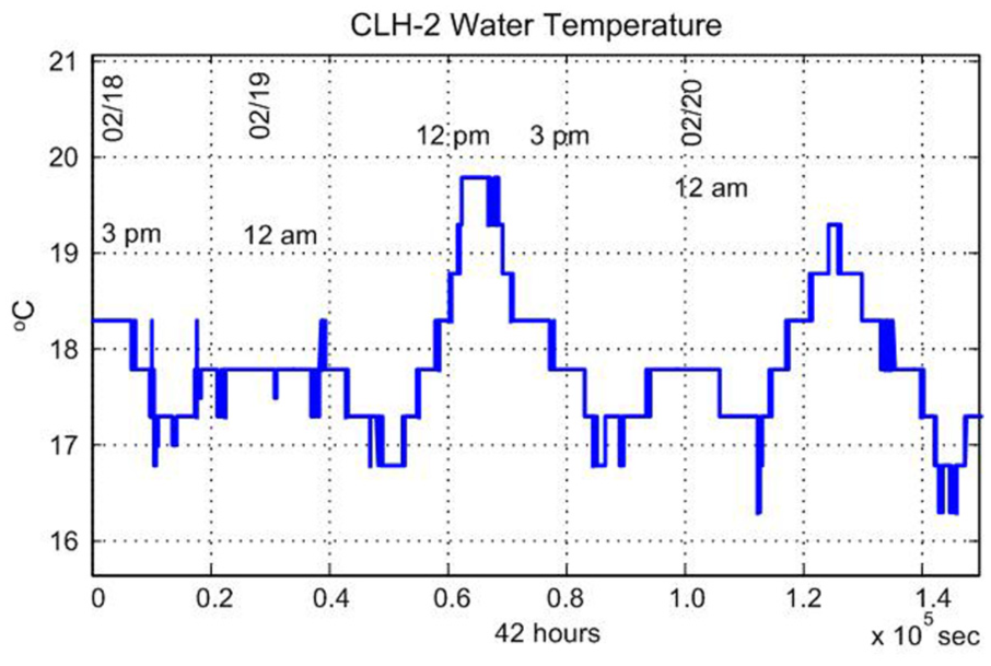
CLH-2 water temperature measurements.

Another important sea water parameter is pH; Figure 17 shows CLH-1 pH measurements. By comparing the temperature variations with pH changing values, it can be corroborated that pH decreases when the water temperature increases and vice versa. Usually, ocean water pH should be above 8 and below 8.8;³⁵ in this case, the maximum registered pH value was 8.51 and the minimum pH was 8.37, within expected parameters.

Figure 17.

CLH-1 pH measurements.

CLH-2 salinity measurements are shown in Figure 18. Similar to pH, salinity changes with temperature (and with ocean water circulation and its tide). Salinity decreases when temperature rises and vice versa. Also, in Figure 18, it is apparent that an event occurred during these trials shortly after 02/20, when the salinity probe was disconnected. After retrieving the equipment, it was evident that something pulled off the probe. Taking into account that the corresponding conductivity electrode was immersed dangling below the water’s surface, it is possible that some kind of water life or fish mistook it as its prey (or its food).

Figure 18.

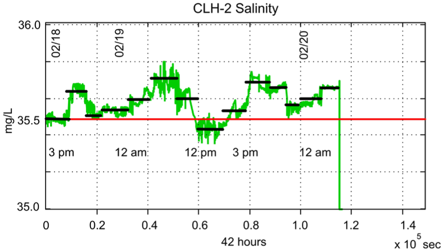
CLH-2 salinity measurements.

This experience served as a reminder that wild life can interfere in experiments where sensors are placed in circumstances that have to be considered to prevent equipment damage. In this case, next time around, the electrode will have to be encased in a more rigid setup to avoid mistaking electrodes as bait.

TRH transmission power control trial results and performance

Figure 19 illustrates CLH-2 air temperature measurements, and Figure 20 shows CLH-2 relative humidity readings. These variables are required by the TRH-TPC algorithm. This algorithm aims to regulate transmission power according to the wireless channel weather conditions and by given RSSI maximum and minimum set points.¹⁹ In this case, we chose −75 and −85 dBm values for CLH-2 TPC maximum and minimum set points. In Figure 21, CLH-1 and CLH-2 transmission power levels are shown. While CLH-1 was configured to transmit at a fixed 600 mW power level, CLH-2 transmission power levels changed according to the TRH-TPC algorithm, reaching a 518 mW average.

Figure 19.

CLH-2 air temperature measurements.

Figure 20.

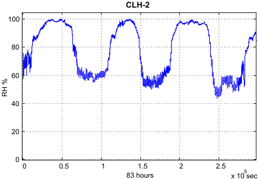
CLH-2 air relative humidity.

Figure 21.

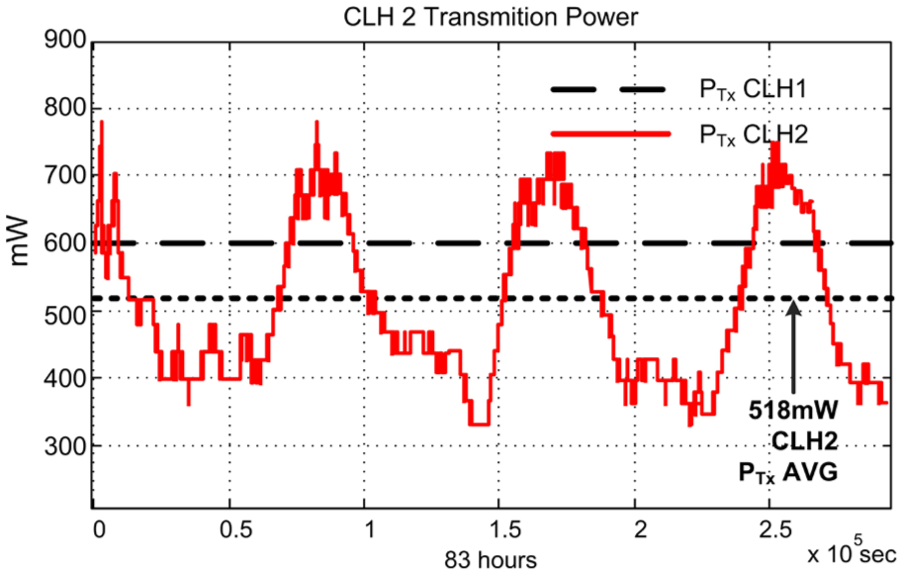
CLH-2 transmission power controlled values versus CLH-1 fixed 600 mW Tx power level.

Although at times CLH-2 transmitted at higher Tx power levels than that of CLH-1 (as shown in Figure 22), the benefits can be seen by comparing the resulting PRRs. Figure 23 shows that CLH-1 averaged a 73.2% PRR. Meanwhile, Figure 24 illustrates the resulting CLH-2 PRR, which obtained a 96.3% average. This means that CLH-1 lost 23.1% more packets than CLH-2, due to CLH-2 use of TRH-TPC. Also, in Figure 24, at different times, deep fading occurred and the non-controlled node’s PRR dropped as low as 4%.

Figure 22.

Base station measurements of received signal strength from CLH-1 and CLH-2.

Figure 23.

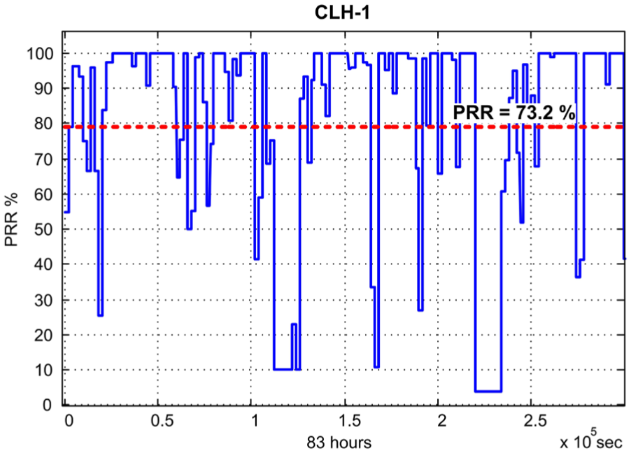
Non-TPC CLH-1 packet received rate, with a 73.2% average.

Figure 24.

TRH Tx power controlled CLH-2 packet received rate, with a 96.3% average.

On the other hand, as previously mentioned, each CLH is provisioned with a solar panel, charge controller and 12 V battery; this setup powers each of the CLH nodes electronic systems: the microcontroller board, the sensor interface shield and the long-range upper-tier radio (which could consume up to 1 W during transmissions). During the day, the solar panels provide electrical current that charge the onboard battery. When there is no sun light, at night and early morning hours, the solar panel doesn’t generate electricity and it is when the battery charge decreases constantly. Comparing charge performance, Figure 25 shows CLH-1 Vin voltage and Figure 26 shows the measured CLH-2 Vin level. CLH-1 had poor performance at night and its battery died a couple of times during morning hours, and this happens to the CLH systems when Vin falls near 7 V.

Figure 25.

Non-TPC CLH-1 battery charge with a solar panel.

Figure 26.

TRH-TPC CLH-2 battery charge with a solar panel.

It is worth remembering that CLH-1 transmits at a fixed 600 mW transmission power, while CLH-2 is the node on which the TRH-TPC scheme operated, and its transmission power varied according to the TRH-TPC behaviour. In general, CLH-2 consumed much less than 500 mW at night; this is apparent in Figure 21. And although CLH-2 consumed almost 800 mW during the day, the surplus solar panel current kept charging the nodes battery. All the while, CLH-1 transmitted at a non-optimum level that depleted its battery charge.

Another possible reason for battery charging problems was due to wild sea life interference, as mentioned before and shown in Figure 13, in which it is evident that seabird guano was dumped on the solar panel surface. Although CLH-1 had the biggest solar panel, it still had power problems at night due to battery depletion during transmissions.

BS solar power generation performance

Here, we present BS solar power generation results, particularly the DC/AC performance. In Figure 27, we show the generated instantaneous direct current; while Figure 28 shows the direct current plotted as a histogram, reflecting the amount of generated current per hour. This direct current was consumed by the inverter that delivers the corresponding AC power to the load and which is plotted as a histogram in Figure 29.

Figure 27.

DC current consumed by the AC inverter operating during 166 h.

Figure 28.

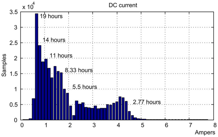
DC current generation histogram during 166 h.

Figure 29.

Base station AC power generation histogram, 144-h operation.

It is apparent in Figure 29 that during 64 h, the inverter delivered an average of 33 W to the AC load, with a 30 W minimum and a 65 W maximum level.

In general, the BSs 33 W AC power average represents 11% of the total inverter’s capacity. This amount of power against its maximum was our aim from the start, and it couldn’t be avoided in any other way because this type of inverter requires this minimum amount of DC current to operate adequately.

Conclusion

In this work, we deployed a 6-day trial of a solar-powered WSN BS along with two long-range marine sensor nodes, placed in the middle of Bahia Falsa’s main canal, on a raft owned by an oyster farm concession. We reported corresponding wireless sensor node deployment results and measured sea water parameters (such as temperature, pH and salinity). Besides sensor system testing, we also tested a transmission power control algorithm that uses a temperature and relative humidity gain controller. This TRH-TPC scheme, operating in harsh marine conditions, outperformed a fixed high power transmission approach, by more than 20% PRR. We also deployed a solar power energy generation system to enable indefinite WSN BS operations, with added wireless performance monitoring features. The corresponding AC load consumed at least 11% of the total power generating capacity. This means that it still has 89% power capacity remaining in ideal conditions.

From the measured sea water quality values, interesting observations can be made, for instance, the water temperature is higher than usual; with the pH data, it is obvious that the closed bay is more alkaline than that of typical open sea values, and its salinity is also high, especially during low tide events. And finally, until a real deployment is done, other non-expected events pertaining to the sea-life activity appears evident, which affects the nodes operation due to sensor tampering.

Footnotes

Academic Editor: Jian Peng

Declaration of conflicting interests

The author(s) declared no potential conflicts of interest with respect to the research, authorship and/or publication of this article.

Funding

The author(s) disclosed receipt of the following financial support for the research, authorship, and/or publication of this article: This work was supported by the Program for Faculty Professional Development known as PRODEP (“Programa para el Desarrollo Profesional Docente”) of the Secretariat of Public Education of México (SEP, “Secreataría de Educación Pública”), under grant IDCA 6692, code UABC-CA-142, project name: “Implementación de una Red de Sensores para Zonas de Cultivo de Ostión en la Bahía Falsa, San Quintín, B.C.”; also received funding from the Autonomous University of Baja California or UABC (“Universidad Autónoma de Baja California”), grant code 300/6/C/15/15 under the name “Redes inalámbricas de sensores en zonas de cultivos acuícolas de Baja California”. And received additional support from the Technological University of Tijuana known as UTT (“Universidad Tecnológica de Tijuana”).

References

Albaladejo

Sánchez

Iborra

. Wireless sensor networks for oceanographic monitoring: a systematic review. Sensors 2010; 10(7): 6948–6968.

Shen

Wang

Applications of wireless sensor networks in marine environment monitoring: a survey. Sensors 2014; 14(9): 16932–16954.

Pelc

Fujita

RM.

Renewable energy from the ocean. Mar Policy 2002; 26(6): 471–479.

Chalasani

Conrad

. A survey of energy harvesting sources for embedded systems. In: IEEE Southeastcon, Huntsville, AL, 3–6 April 2008. New York: IEEE.

Bader

Oelmann

Durable solar energy harvesting from limited ambient energy income. Int J Adv Netw Serv 2011; 4(1–2): 66–80.

Huso

Dietsch

Chris

Mortality monitoring design for utility-scale solar power facilities. Open-File Report 2016-1087. US Department of the Interior, US Geological Survey, 2016, https://pubs.usgs.gov/of/2016/1087/ofr20161087.pdf

Chu

Meisen

Review and comparison of different solar energy technologies. San Diego, CA: Global Energy Network Institute (GENI), 2011.

Mason

SP.

Atmospheric effects on radio frequency (RF) wave propagation in a humid, near surface environment. Monterey, CA: Naval Postgraduate School, March2011.

Karagianni

Mitropoulos

Latif

. Atmospheric effects on EM propagation and weather effects on the performance of a dual band antenna for WLAN communications. J Nav Sci Technol Part B: Electr Eng Comput Sci 2014; 5: B-29–B-45.

10.

Rawat

Singh

Chaouchi

. Wireless sensor networks: a survey on recent developments and potential synergies. J Supercomputing 2014; 68(1): 1–48.

11.

Cella

Shuley

Johnstone

. Wireless sensor networks in coastal marine environments: a study case outcome. In: Proceedings of the fourth ACM international workshop on underwater networks (WUWNet ‘09), Berkeley, CA, 3 November, Article no. 8. New York: ACM.

12.

Anastasia

Conti

Di Francescoa

. Energy conservation in wireless sensor networks: a survey. Ad Hoc Netw 2009; 7(3): 537–568.

13.

Khana

Qureshia

Iqbalb

Energy management in wireless sensor networks: a survey. Comput Electr Eng 2015; 41: 159–176.

14.

Zyruanov

VN.

Physical properties of seawater, including its three phases. Types and properties of water – vol. 1. UNESCO. Encyclopedia of Life Support Systems, 2009, http://www.eolss.net/sample-chapters/c07/e2-03-03-01.pdf

15.

Onset Computer Corporation. HOBOnode outdoor wireless system. User’s guide, 2009–2012, http://www.onsetcomp.com/files/manual_pdfs/12473-K%20MAN-HOBOnode-UG.pdf (accessed September 2016).

16.

Onset Computer Corporation. HOBOnode outdoor repeater, 2011, http://www.onsetcomp.com/files/manual_pdfs/12474-D%20MAN-W-REPEATER-QS.pdf (accessed September 2016).

17.

Ortega-Corral

Palafox

Garcia-Macias

. End-to-end message exchange in a deployable marine environment hierarchical wireless sensor network. Int J Distrib Sens N 2014; 2014: 950973 (18 pp.).

18.

Ortega-Corral

Palafox

Garcia-Macias

. Transmission power control based on temperature and relative humidity. In: Proceedings of the 9th IEEE international conference on intelligent sensors, sensor networks and information processing (ISSNIP’14), Singapore, 21–24 April 2014, pp.1–6. New York: IEEE.

19.

Ortega-Corral

Palafox

García-Macías

. Parameter optimization of a temperature and relative humidity based transmission power control scheme for wireless sensor networks. Int J Distrib Sens N 2015; 2015: 921319 (23 pp.).

20.

CESAIBC. Fichas técnicas de la Unidad de Producción Acuícola: Granja Ostrícola Nautilus S. de R.L. de C.V. Fichas Técnicas de Productores de Moluscos del Comité Estatal de Sanidad Acuícola e Inocuidad de Baja California (CESAIBC), Mexico, 2012, http://www.cesaibc.org/sitio/archivos/FT_10_%20NAUTILUS_200313160520.pdf (accessed September 2016).

21.

Tapia Vázquez

Hirales

Sáenz Gaxiola

LM.

Sistemas de cultivo para la producción de ostión en Baja California, México. Comité Estatal de Sanidad Acuícola e Inocuidad de Baja California (CESAIBC), Mexico, 2013, http://www.cesaibc.org/sitio/archivos/sistemas_280513123333.pdf (accessed September 2016).

22.

Canua

Aveytua-Alcázara

Camacho-Ibarc

. Hydrodynamic properties of San Quintin Bay, Baja California: merging models and observations. Mar Pollut Bull 2016; 108(1–2): 203–214.

23.

Cassis

Pearce

Maldonado

MT.

Effects of the environment and culture depth on growth and mortality in juvenile Pacific oysters in the Strait of Georgia, British Columbia. Aquacult Env Interac 2011; 1: 259–274.

24.

ICES. Report of the Working Group on Harmful Algae Bloom Dynamics (WGHABD) (ICES CM 2013/SSGHIE:09), 9–12 April 2013, Belfast, 2013, https://www.ices.dk/sites/pub/Publication%20Reports/Expert%20Group%20Report/SSGHIE/2013/WGHABD13.pdf

25.

Office of Water. Impacts of climate change on the occurrence of harmful algal blooms. United States Environmental Protection Agency, EPA 820-S-13-001, May2013, https://www.epa.gov/sites/production/files/documents/climatehabs.pdf

26.

Arduino

LLC

. Arduino mega, http://arduino.cc/en/Main/arduinoBoardMega (accessed August 2016).

27.

RFC4627. JSON: JavaScript Object Notation Standard Specification, http://www.ietf.org/rfc/rfc4627.txt (accessed August 2016).

28.

Ortega-Corral

Palafox

García-Macías

. A lighter JSON for message exchange in highly resource constrained wireless sensor network application. Congr Int Ing Electrón Mem Electro 2012; 34: 73–78.

29.

Digi International. Rabbit core RCM4300 C-programmable analog core module with microSD card storage and Ethernet. User’s manual, 2010, http://ftp1.digi.com/support/documentation/019-0163_J.pdf

30.

Laird Tech. AC4490 900MHz transceiver user’s manual, version 3.2.1. Bengaluru, India: Laird Tech, 2007.

31.

Laird Tech. AC4490 developer kit user’s manual, version 3.3. Bengaluru, India: Laird Tech, 2005.

32.

Digi International. Dynamic C. Integrated C development system for rabbit 4000, 5000 and 6000 microprocessor. User’s manual. Minnetonka, MN: Digi International, 2011.

33.

Correia

LHA

Macedo

Dos Santos

. Transmission power control techniques for wireless sensor networks. Comput Netw 2007; 51(17): 4765–4779.

34.

Delgado-González

Marván-Gargollo

Mejía-Trejo

. Chapter 6. San Quintín lagoon hydrodynamics case study. In: Nayak

(ed.) Water resources management and modeling. InTech Open, 2012, pp.127–144, DOI: 10.5772/2067.

35.

McCaffrey

Catchment

Water quality parameters and indicators. Water Watch, New South Wales; Office of Environment and Heritage, 2010, http://www.sswm.info/sites/default/files/reference_attachments/MCCAFFREY%20ny%20Water%20Quality%20Parameters%20&%20Indicators.pdf (accessed August 2016).

Lessons learned deploying an oyster farm monitoring auto-sustainable wireless sensor network and trial of a temperature and relative humidity–based transmission power control scheme

Abstract

Keywords

Introduction

Background and related work

Oyster farm end-to-end telemetry architecture

WSN upper-tier implementation

WSN application messages

BS gateway and co-state operations

TRH transmission power control

Experimental setup

Auto-sustainable WSN BS

Deploying water quality monitoring on a seaworthy floating vessel

pH and salinity probe and their interface with the wireless nodes

Combined results and comments

Water quality sensor readings

TRH transmission power control trial results and performance

BS solar power generation performance

Conclusion

Footnotes

Declaration of conflicting interests

Funding

References