Distributed Time Division Pattern Formation for Wireless Communication Networks

Abstract

This paper proposes a novel communication timing control for wireless sensor networks, named Phase Diffusion Time Division method. This is based on the mutual synchronization of coupled phase oscillatory dynamics with a stochastic adaptation, according to the history of collision frequency in communication nodes. Through local and fully distributed interactions in the communication network, the coupled phase dynamics self-organizes an efficient time division pattern of the communication so that the network reduces the collision frequency by diffusion of the phase pattern, while it sustains sufficient throughput of the communications. We introduce the built-in virtual node dynamics model for sensor device, to implement impulse signal based interactions. This method is designed for applications in a regular grid model of the wireless network, but it can be extended to an irregular grid model as simulation results illustrate, where the proposed method outperforms CSMA method in the efficiency.

1. Introduction

In recent years, research on wireless sensor networks has been promoted rapidly [1]. The sensor network is composed of distributed sensor devices connected with wireless communication and sensing functions. Potential application fields of the sensor network include stock-management systems, road traffic surveillance systems, and air-conditioning control systems of a large-scale institution and so on. There are many technical issues in the sensor network. One of them is a communication timing control. In order to cope with malfunctions and changes of the number of active sensor nodes, a distributed autonomous communication timing control is preferable to centralized approaches which must rely on the fixed base stations in general. Another important issue is related to energy saving. Downsizing a device is an essential problem. In radio communications, it is known that the transmitted electrical power consumption increases in proportion to the 2–4th power of the transmission distance [2]. Therefore, compared with distant one-hop communication, rather short distance communication by multi-hop communication has a merit from the viewpoint of electrical energy saving. However, short distance multi-hop communication increases the number of data packets, so collision probability becomes high.

In order to avoid the collision issue, TDMA [3] system has been presented, which is a multiplexing technology in the time domain and makes it possible to avoid collisions by assigning a communication slot to each node to one frame. So there is no collision of communication, and any node can obtain an impartial communication right in TDMA system. Thereby TDMA is widely used in a cellular telephone system. However, TDMA is fundamentally a centralized management technique depending on a base station and is applicable to a star link network. Meanwhile, distributed slot assignment TDMA approach for ad hoc networks is proposed. In Ephremides and Truong algorithm [4], allocation of one transmission slot is assured for each node by preparing N slots for N nodes. In addition, it is possible to add more slot allocations by referring to the information of slot allocation within the two hop nodes for the collision avoidance base on a distributed algorithm. However, it is necessary to know the total number of the nodes beforehand, and has some limitations to change the number of nodes flexibly. USAP-MA [5] deals with a distributed slot assignment in TDMA for changes of the number of nodes. This method provides a dynamic change of frame length corresponding to the number of nodes and network topology. As a result, this method improves bandwidth efficiency. Also the other method of slot reservation is proposed for TDMA [6], [5], [7]. These methods are based on TDMA and provide a distributed slot assignment, but the TDMA based approach requires the global time synchronization.

Several media access controls for these demands have been developed so far, such as ALOHA [8], MACA [9], FAMA [10], etc. CSMA [11], [12] is the most widely used protocol in the standard wireless LAN. However, with the increase of nodes, communication throughput sharply declines due to frequent collisions of the packets. Such a collision should be avoided not only for improvement of the throughput efficiency, but also for saving the electrical energy consumption required for retransmissions. Furthermore, several problems are pointed out as to the costs of carrier sense [13] and hidden terminals [11], [12]. Also, the CSMA based approach makes it difficult to ensure impartial communication correctly, because of the contention of nodes that shares the communication channel. Some other research for collision avoidance in wireless sensor networks includes SMAC [14], SMACS [15]. SMAC is based on CSMA, where each node broadcasts a sleep timing schedule to the neighbor nodes. So the nodes receiving this message are to adjust the schedule for sleep and waking time, by which the node can save energy consumption. SMACS realizes an efficient communication based on a synchronization between two certain nodes corresponding to a certain link. These nodes attempt to schedule a communication timing with each other. Additionally, each node utilizes a different frequency for a different link for collision avoidance. In this method, the risk of collisions becomes small by random sharing of the frequency band. This method is different from the basic TDMA in that synchronization is required between the two corresponding nodes while TDMA requires global synchronization. In general, global synchronization without a base station is hard to achieve. Although the problem of collision is an inevitable question, the aim of the above research is focused on a timing control for saving energy consumption. Fundamental problems in CSMA remain unsolved. In this paper, our concern is to make more efficient use of the limited band in the wireless communication in the sensor network, spatially and temporally. So, we propose a novel communication timing control method for the wireless sensor network, named Phase Diffusion Time Division method (PDTD). Unlike the conventional protocols based approaches, this method is based on the dynamics of mutual synchronization with stochastic adaptations. Through the local interactions among the sensor nodes, an efficient communication timing pattern is self-organized to reduce the collision frequency. This realizes collision-free communication in high traffic wireless networks without any base station.

2. Phase Diffusion Time Division Method

A. Phase Dynamics and Synchronization

In this section, we first address a brief introduction on the phase dynamics to make it more accessible to the readers who may not be familiar with the concept. A more thorough introduction is available in reference [16].

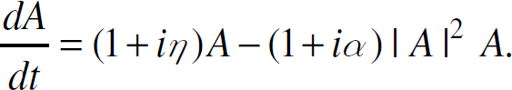
Nonlinear oscillation is a phenomenon which is widely observed in almost every field as seen in biophysics, chemical reaction, electric circuit, aerodynamics, or population dynamics as well as in many engineering systems modeling. Such a nonlinear dynamics often exhibits a complex and emergent behavior, called self-organization and such properties have been explored to apply to several engineering techniques as a new approach. One of the most basic and typical behavior of nonlinear oscillation is probably a limit-cycle, which has a self-sustained and periodic attractor with structural stability. The structural stability means properties that a solution of the dynamics remains stable against some degree of disturbance. Such behavior is often referred to as nonlinear oscillator dynamics, or simply an oscillator. Nonlinear oscillator is originally described in the form of a nonlinear ordinary differential equations with actual physical or system variables, but the dynamics is often reformed to a canonical form of complex amplitude equation for mathematical analysis, which is typically given by the following form,

$$\frac{dA}{dt}=(1+i\eta )A-(1+i\alpha )|A{|}^{2}A.$$

(1)

$A(t)=r(t{)}^{i\theta (t)}$ is a complex variable, where r is the amplitude, θ is the phase, ŋ and α are some constant real number, and i is imaginary number. By substituting A = re^iθ into eq.(1) and comparing the corresponding part, one can easily confirm that eq.(1) is divided into the part of amplitude and phase dynamics as given by,

$$\frac{dr}{dt}=r(1-r^2),$$

(2a)

$$\frac{d\theta }{dt}=\eta -\alpha r^2.$$

(2b)

Since eq.(2a) is stable and r(t) will converge to r = 1, the coupled dynamics will reduce to only the phase dynamics of eq.(2b) in the end. Hence, in a simple description of the oscillator model, we often deal with only the part of phase dynamics with some extended form. The systems composed of two or more interactive oscillators may exhibit an emergent phenomena of mutual synchronization or entrainment as observed in a number of fireflies, cardiac muscle cells, and brain cells activities, etc. In spite of different frequency and initial phase values, the coupled oscillators may exhibit a phase locking under some conditions. One of the standard models for mutual syntonization is the Kuramoto model [17], which is known to have first appeared in simple phase dynamics to deal with mutual syntonization. In the case of a mutual synchronization of weakly coupled oscillators, a typical form is described as follows,

$$\frac{d{\theta }_1}{dt}={\omega }_1+K_1\sin ({\theta }_2-{\theta }_1),$$

(3a)

$$\frac{d{\theta }_2}{dt}={\omega }_2+K_2\sin ({\theta }_1-{\theta }_2).$$

(3b)

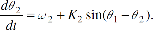
Where, ω₁ and ω₂ are referred to the natural frequency or the eigenfrequency, and K₁ and K₂ are positive constant. Subtracting eq.(3a) from eq.(3b) give the dynamics of phase difference Δθ₁₂ = θ₂ − θ₁, which is given by,

$$\frac{d\mathrm{\Delta }{\theta }_{12}}{dt}={\omega }_2-{\omega }_1-(K_1+K_2)\sin (\mathrm{\Delta }{\theta }_{12}).$$

(4)

Eq.(4) has a stable fixed point under the condition that the difference between eigenfrequency ω₁, ω₂ is sufficiently small and the coefficient is large enough. Thus, if the phase lock is realized, eq.(3a) and (3b) are synchronized with a different frequency from the initial eigenfrequency. The general discussion is more complex, but it is extended to the case of a large number of coupled oscillators. The basic synchronization mechanism has been applied to several engineering systems as well as to a communication technique, among which is the well known PLL (Phase Locked Loop) [18]. PLL exploits a phase dynamics for synchronization of the communication signals. Since largely coupled PLL systems exhibit complex behaviors, it has also been applied as a platform to examine a nonlinear complex behaviors.

In this paper, we exploit the coupled phase dynamics for collision avoidance in wireless communication. It should be stressed that we do not apply the above mentioned theory in a straightforward manner. According to eq.(3a) and (3b), the phase difference will take zero if eigenfrequency is equivalent to each other. It suggests that a communication timing synchronization and collision may occur. Instead, we introduce a specific repulsive phase response function to avoid a collision as well as achieving phase locking for efficient communication timing pattern.

B. Phase Pattern Formation for Collision Avoidance

Assume a situation where a number of communication nodes (which may be more than hundreds to thousands of nodes) are assigned in the grid form as shown in Fig. 1. Each node is numbered for reference of the problem descriptions, but our method does not rely on the node ID explicitly. The small circles depicted as R₁, R₃, R₈ suggest the communication range of the corresponding node 1, 3, and 8. Communication range means conventional data transmission range of the node. There is an interference range to obstruct the communication of other nodes when the node communicates within the range of R. This interference range is larger than the communication range. However, we simplify the condition that the collision is caused by, by overlapping of the communication range in this paper. (The interference problems will influence on the following discussion, however the overall arguments will essentially hold with a slight modification. So, we will not deal with every detail of the problem to avoid further complication in this stage.) Then, the range where the nodes are related to the collision is defined as the range of 2R. In this paper, we call this range as the interaction range. In Fig. 1, the larger circle 2R₁ indicates the interaction range from the node 1. In the interaction range, there are nodes that will require the communication timing adjustment for the collision avoidance. In these sensor networks, suppose that each node communicates with adjacent nodes in a relatively high frequency. (Conventional sensor network assumes very low frequency of communication.) Our aim is to realize an efficient timing control of the communication under these conditions without any global surveillance or scheduling. Apparently, the conventional CSMA has difficulty in dealing with this problem, because so many collisions will occur. Unlike protocol based schema, the PDTD method is based on a stochastic adaptation of the coupled phase oscillatory dynamics. In this method, a specific repulsive phase dynamics is designed in each node, where eigenfrequency is assumed to be the same with each other. (We can synchronize the frequency if it is different, so this assumption is a mild constraint.) The phase of oscillator for each node i is denoted as θ _i , and we suppose that each node can transmit the data only within the phase interval of 0 ≤ θ _i < ϕ _c as depicted in Fig. 2. Out of the phase interval, the node can receive a signal as long as no collisions are detected. The dynamics of PDTD self-organizes an efficient phase difference pattern to eliminate potential collisional states from randomly assigned initial phase distribution in the network. In Fig. 1, node 1 can communicate with nodes {0,5,6,10}, but the collision may occur unless the phase difference is smaller than the phase margin of ϕ _c . Node 0 is a potential hidden terminal between node 1 and 3, as well as node 2 and 4, although these nodes will not directly collide with each other. Therefore, the phases of node 1 and 3 should be apart from each other. From these observations, we can see that every phase of the nodes within the range of 2R₁ should be sufficiently kept away from the phase of node 1, while every node i also must adjust its peripheral phase constraint in the range of 2R_i. Hence, it should be noted that randomly diffused phase patterns are easily realized, but are inefficient as well. A set of phases of the node which will not collide with each other are desired to cluster and these clusters of the phase are efficiently divided to improve the time division pattern. According to Fig. 1, it can be seen that a collision will not take place during the relation between node 1 and 8, as well as node 11, which is located out of the interaction range 2R₁. So these phases can be synchronized and made into a cluster, although there is no direct interaction. The optimal phase pattern formation corresponding to this observation is depicted in Fig. 3, where a randomly assigned phase pattern is reformed to a set of clusters with the collision free state. Through the dynamics of PDTD, each node forms the phase difference appropriately to avoid collisions, by which the communication can be guaranteed at a fixed cycle without a waiting loss.

FIGURE 1

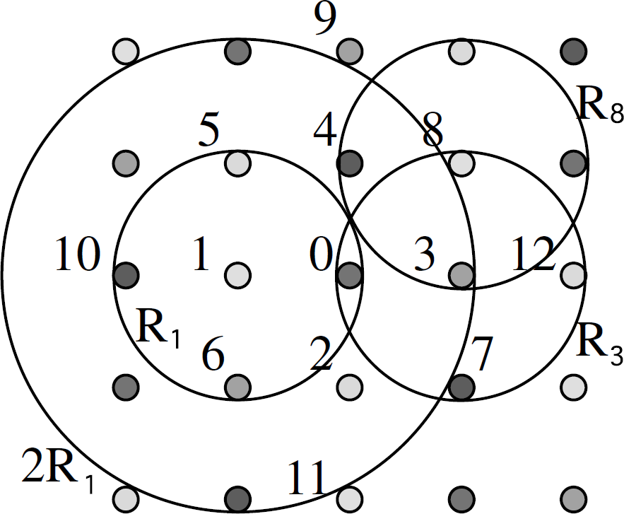
Node arrangement and communication range.

FIGURE 2

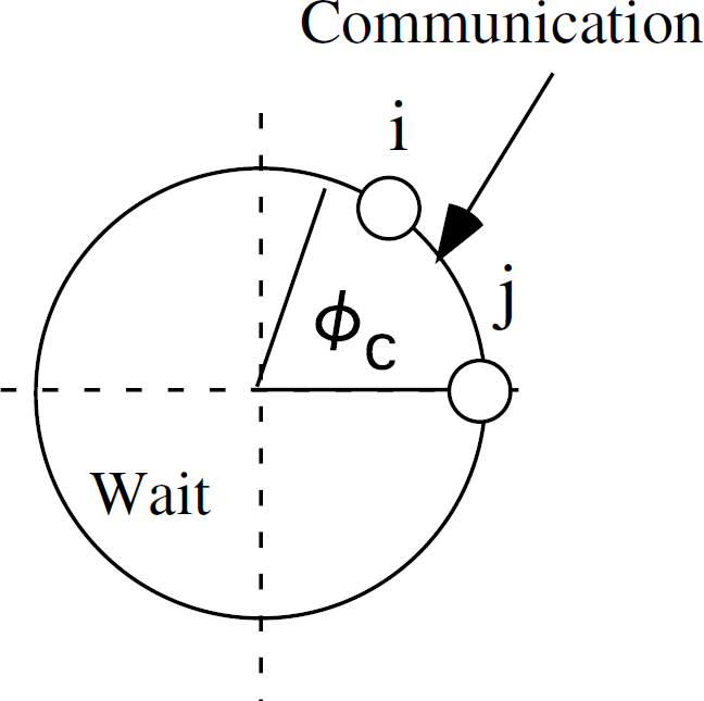
Phase expression of communication timing.

FIGURE 3

Formation of phase difference.

C. Definition of Collision and Collision Rate

PDTD is a communication timing control method based on a stochastic adaptive dynamics reflecting the history of collisions. It is required to evaluate collision detection as to whether an effective phase pattern is formed or not. However, it is generally difficult to detect collisions in the wireless communications. Therefore, we introduce an estimation of the collision by phase difference with the other nodes. Although this is not a real collision of the actual communication, it is useful to predict possible collisions. In this section, we first define the collision and collision rate as an index to evaluate the performance of communication timing control. In general, collisions will occur in the following situations.

When node i attempts to communicate during any node in the communication range R_i is sending a data.

As shown in Fig. 4, if node 1 and 3 attempt to communicate with node 2 at the same time, the collision with node 2 occur, but nodes 1 and 3 do not recognize the collision. This is called the hidden terminal problem as we mention in the previous section.

FIGURE 4

Collision of hidden terminal.

So, when the radius of communication range is R, it is necessary to notice states of the nodes located in the range of 2R, which we call the interaction range. Each node must consider communication timing adjustment with the nodes in the interaction range. Now, the collision is formally defined as follows.

D. Definition of Collision

Definition of the collision is based on phase value of the nodes inside of the interaction range. So, the collision detection is different from that of the wired networks. For collision detection, the node state Q is introduced by,

$$Q=\{\mathit{\text{Wait}},\mathit{\text{Communication}},\mathit{\text{Collision}}\}.$$

(5)

Hence, Wait is a standby state for a communication, Communication is a state for a data transmission, and Collision is a state where a collision is detected. Every node takes one of these states. According to phase θ _i at time t, a communication flag function for a state transition in Q is defined as

$$O_i({\theta }_i(t))=\{\begin{array}{l}1\hspace{0.17em}\hspace{0.17em}\hspace{0.17em}0\le {\theta }_i<{\varphi }_c,\\ 0\hspace{0.17em}\hspace{0.17em}\hspace{0.17em}\hspace{0.17em}{\varphi }_c\le {\theta }_i<2\pi .\end{array}$$

(6)

O_i switches the node state between Communication and Wait. In case of O_i = 1, the node state will be changed to Communication from Wait, and in case of O_i = 0, it will be changed to Wait from Communication or Collision. The state Collision is determined by the collision flag function x_i. Let K_i be a set of nodes in the interaction range 2R of the node i. Then, the collision flag function is defined as follows,

$$x_i^{\prime }(t)=\{\begin{array}{ll}1& O_i({\theta }_i)=1,\text{and}{\sum }_{j\in K_i}{O}_j({\theta }_j)>0,\\ 0& \text{else}.\end{array}$$

(7a)

$$x_i(t)=\{\begin{array}{ll}1& \text{if\hspace{0.17em}}{O}_i({\theta }_i)=1,\text{and}D({\theta }_i,\mathrm{\Theta })<{\varphi }_c\\ 0& \text{else}.\end{array}$$

(7b)

$$D({\theta }_i,\mathrm{\Theta })=\{\begin{array}{ll}2\pi -|\mathrm{\Theta }-{\theta }_i|& (|\mathrm{\Theta }-{\theta }_i|>\pi ),\\ |\mathrm{\Theta }-{\theta }_i|& (|\mathrm{\Theta }-{\theta }_i|\le \pi ).\end{array}$$

(8)

Where, the collision flag function is defined in two ways, such as $x_i^{\prime }(t)$ and x_i(t). Eq.(7a) is a rigorous evaluation for the collision detection based on continuous monitoring of the phase. This flag function implies a collision if node i takes the state Communication with interaction nodes at the same time, and we use it for simulations to evaluate collision states. However, each node cannot observe the phase of the neighboring node continuously in the actual wireless communications, so it is difficult to apply this formula directly, because we assume that a pulse signal is employed for inter-node interactions, so it is hard to monitor the phase of the other nodes continuously. Therefore, we modify Eq.(7a) to Eq.(7b), which is employed in the actual nodes. Where, function D(θ _i , Θ) indicates the phase difference between θ _i and Θ. When node i receives a pulse signal, the phase of the node which transmitted the pulse signal is set to Θ. Fig. 2 depicts a collision state, where the phase of node j becomes 0, and the node transmits a pulse signal. (We assume that the pulse signal is transmitted in case that phase value is 0.) In this case, the state of node i is Communication, then node i counts the collision. We neglect a case of duplicated collisions, and they are counted as one collision since it is not influential to the performance of the method. The state Collision will transit to Wait when O_i = 0 regardless of the other node states. The above mentioned node state transitions are summarized in Fig. 5.

2) Definition of Collision rate. In order to evaluate the efficiency of the communication network, we define a collision rate, which is based on the history of collisions. Let γ be the number of transitions to Collision detected by eq.(7a) in the past nT_i seconds, and also let γ be the number of transitions to Collision by eq.(7b). Where, $T_i=\frac{2\pi }{{\omega }_i}$ is the cycle and ω _i is the natural frequency of node i respectively. The collision rate is defined as a ratio of the recorded number of collisions for the number of the maximum collision times. Since node i communicates once per cycle, the number of the maximum collision times is n. Therefore, the collision rate is given by,

$$c_i^{\prime }(t)=\frac{{\gamma }^{\prime }}{n}$$

(9a)

$$c_i(t)=\frac{\gamma }{n}$$

(9b)

FIGURE 5

Node state transition diagram.

Eq.(9b) is a self evaluation index. Each node implements a stochastic search by this evaluation, while, Eq.(9a) is a system evaluation index which is used in the evaluation of simulation results. Hence, the frequency of each node generally fluctuates due to the phase dynamics described in the next section, so the cycle T_i is updated in every cycle. Since T_i is adopted from the previous cycle, the current actual cycle may be smaller than T_i, which may cause a case of c_i ≥ 1, but we regard c_i = 1.0 in such a case. This simplification is satisfactory as long as the fluctuation of the cycle is not very large and this is a normal situation in our model. Then c'_i is exploited for the stochastic adaptation of the dynamics.

D. Coupled Stochastic Phase Dynamics

The oscillator of node i interacts with nodes in the interaction range, and the time evolution of the phase dynamics is described by stochastic coupled oscillator dynamics. Where the stochastic term ξ(S_i) is adaptive to reduce the collision rate c_i. Let θ _i (t) (0 ≤ θ _i < 2ర) be the phase of node i at time t. The phase difference between node i and node j is given by Δθ _ij = θ _j – θ _i , (mod 2ర). Then, the coupled phase dynamics is introduced as follows,

$$\frac{d{\theta }_i}{dt}={\omega }_1+\frac{k}{N_i}\sum _{j\in K_i}\hspace{0.17em}R(\mathrm{\Delta }{\theta }_{ij})+\xi (S_i).$$

(10)

Where, ω _i is the eigenfrequency of the oscillator, K_i is a set of nodes in the interaction range 2R_i, and N_i is the number of elements in K_i. k is a coupling coefficient. R(Δθ _ij ) is a phase response function and ξ(S_i) is a stochastic function. Function R(Δθ _ij ) determines interaction value. This function is a repulsion function with interaction nodes to form an effective phase difference. Only during repulsion of each node, there is no sequence change in phase space. Sequence of nodes in phase space is important to form effective phase pattern. Hence, the stochastic function ξ(S_i) causes a random change to the phase value to change a sequence of the nodes in the phase space appropriately.

1) Phase Response Function

As we discussed in 2-B, the purpose of interactions is the generation of a collective dynamics to realize the following effects. (See Fig. 3 again.) (i)

For collision avoidance with nodes in the interaction range, the phase diffusion must be realized through the repulsive action in the phase dynamics.

A set of phases of collision-free nodes are desired to synchronize in order to reduce unnecessary phase diffusion to improve potential throughput of the communications.

The phase response function R(Δθ _ij ) to achieve such a phase pattern is defined as follows,

$$R(\mathrm{\Delta }{\theta }_{ij})=\{\begin{array}{ll}\alpha \cdot (\mathrm{\Delta }{\theta }_{ij}-\frac{2\pi }{p})& \mathrm{\Delta }{\theta }_{ij}\le \frac{2\pi }{p},\\ \beta \cdot \mathrm{\Delta }{\hat{\theta }}_{ij}& \frac{2\pi }{p}<\mathrm{\Delta }{\theta }_{ij}<2\pi -\frac{2\pi }{p}\hspace{0.17em}and\hspace{0.17em}\mathrm{\Delta }{\hat{\theta }}_{ij}<\frac{\pi }{p},\\ \beta \cdot (\mathrm{\Delta }{\hat{\theta }}_{ij}-\frac{2\pi }{p})& \frac{2\pi }{p}<\mathrm{\Delta }{\theta }_{ij}<2\pi -\frac{2\pi }{p}\text{\hspace{0.17em}and\hspace{0.17em}}\mathrm{\Delta }{\hat{\theta }}_{ij}>\frac{\pi }{p},\\ \alpha \cdot (\mathrm{\Delta }{\theta }_{ij}-\frac{(p-1)\pi }{p})& 2\pi -\frac{2\pi }{p}\le \mathrm{\Delta }{\theta }_{ij}.\end{array}$$

(11)

$$\beta =u(1-c_i{)}^2.$$

(12)

FIGURE 6

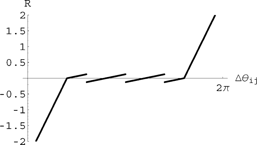
Phase response function (case p = 5).

Where, $\mathrm{\Delta }{\hat{\theta }}_{ij}=\mathrm{\Delta }{\theta }_{ij}$ (mod $\frac{2\pi }{p}$ ), and α, v are constant coefficient. Also p denotes the number of phase divisions, which must be chosen to satisfy $\frac{2\pi }{p}>{\varphi }_c$ so that a sufficient large phase margin is guaranteed for a collision free phase pattern. A typical shape of R(Δθ _ij ) is shown in Fig. 6. The situation depicted in Fig. 3 is an ideal case, and there is no redundancy in the phase division. This is difficult to realize in a fully distributed approach based only on the local interactions. However, by choosing a sufficiently large p, an efficient phase pattern can be formed as the following simulation results will illustrate. We also note that eq.(12) is responsible for the stochastic adaptation, where the slope of R(Δθ _ij ) changes according to the collision rate ci. At the initial stage of adaptation, where the collision rate may be high ( $c_i\simeq 1$ ), the middle part of the phase response function eq.(11) is nearly flat, where the phase diffusion for collision avoidance should be prior to forming a phase division pattern of clustered nodes. However, after the collision avoidance is attained (c_i → 0), then the slope of the middle range of the function grows in order to facilitate an effective phase difference pattern to maintain the communication throughput.

2) Stochastic Adaptation

As we can see from Figs. 1 and 3, since a spatial node allocation (network topology) is very influential to the optimal phase pattern, the sequence of the phase pattern must be permutable from the initial phase pattern. However, a continual time evolution by the phase response function cannot cope with the permutation of the phase pattern. Therefore a stochastic fluctuation reflecting the collision rate is incorporated into the dynamics. For an intuitive understanding, suppose a situation where the phase of node 1 is near the node set comprising of nodes 3, 6, and 9 in Figs. 1 and 3. Then, communication of node 1 will not collide with communication of node 0, but it will collide with node 6 directly, and node 1 and 3 will cause the hidden terminal problem at node 0. Therefore, the phase of node 1 has to move to the set of nodes 8 and 11. However, it is not possible for node 1 to climb the potential barrier made with the phase response function, which prevents node 1 from approaching the phase of nodes 2, 5, and 12. In such a case, node 1 has to jump somewhere between node 0 and 2, by stochastic adaptation.

In order to adjust moderate fluctuations, the stress function s(c_i) is defined to return a steep stress value when the collision rate c_i(t) is especially high, that is,

$$s(c_i)=\{\begin{array}{ll}0& (c_i=0),\\ 0.01& (0<c_i\le 0.9),\\ 0.9& (0.9<c_i).\end{array}$$

(13)

FIGURE 7

Stress function.

The integration of stress S_i for a certain period is given by,

$$S_i={\int }_{t_a}^{t}S(c_i)dt.$$

(14)

Where, t_s is a time when the phase is fluctuated by a stochastic noise ξ(S_i) (ξ(S_i) is described later). Let q(S_i) be a function which returns a random value according to the integrated stress

$$q(S_i)=\{\begin{array}{ll}\mu & \text{with probability\hspace{0.17em}}{S}_i,\\ 0& \text{with probability\hspace{0.17em}}1-S_i.\end{array}$$

(15)

Where μ is a random value in [‒π, π]. If S_i is larger than 1, then we regard S_i as 1. The stochastic fluctuation ξ(S_i) is defined to return a random value in every nT_i second, as follows

$$\xi (S_i)=\{\begin{array}{ll}q(S_i)& \text{if\hspace{0.17em}}t=mn{T}_i(m=1,2,\dots ),\\ 0& \text{elec}.\end{array}$$

(16)

In a normal stochastic differential equation, a diffusion term functions in every continual time, but this stochastic diffusion term functions only in every nT_i cycle. In the initial stage of adaptation, the stochastic adaptation frequently works, but as the collision rate decreases, it ceases to function gradually.

3. Virtual Node Dynamics Model

A. Virtual Node Interaction

In section 2-D, eq.(10) assumes that each node can observe the phase of nodes in the interaction range in real time. However, it is difficult to monitor the phase of the peripheral nodes correctly in general. Also, interactions are based on pulse signals rather than continuous signal. This becomes a drawback for implementation of the theory to the actual hardware device. So, we introduce a virtual node dynamics model, which is a slight extension of the basic model. Where, each node has the phase of peripheral nodes in the interaction range virtually to compensate uncertainty.

B. Virtual Node Model

In the virtual node model, each node has a variable number of virtual nodes for interactions. And each node interacts continuously with a virtual node although the actual interaction is based on the pulse signal. Interactions with a virtual node compensate the difference caused by the pulse signal interactions. Fig. 8 depicts the system configuration for the virtual node model. In Fig. 8, Pulse/Phase converter unit transforms pulse signal to phase Θ. Add virtual node unit controls addition and adjustment of the virtual node from pulse signals. Delete virtual node unit controls deletion of dispensable virtual nodes. Virtual node dynamics unit controls the phase dynamics of virtual nodes. Phase dynamics unit controls the phase dynamics of interactions with virtual nodes. Communication timing controller unit controls actual data communications based on the phase dynamics. Pulse controller unit controls a pulse transmission. In this article, we assume that each node transmits a pulse signal at θ _i = 0. In the virtual node model, each node interacts with virtual nodes which are generated by the pulse signal from its real interaction nodes. And each node calculates the phase dynamics by the phase of virtual nodes, in stead of the phase of peripheral nodes. Details in each unit is explained following subsections.

FIGURE 8

System configuration of Virtual Node Dynamics model.

1) Add virtual node unit

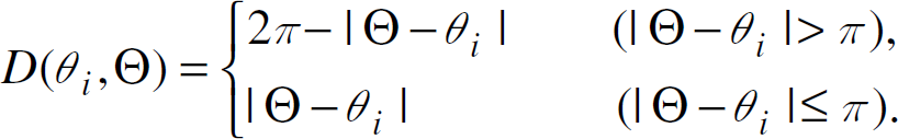
Adding virtual node unit controls the addition and adjustment of virtual nodes from a pulse signal. When each node receives the pulse signal, adding virtual node unit implements addition of a virtual node or adjustment of the phase of virtual node. Addition or adjustment of the node is determined as follows,

$$u=\underset{j\in {\tilde{K}}_i}{\arg min}D({\tilde{\theta }}_{ij},\mathrm{\Theta }).$$

(17)

$$\{\begin{array}{ll}{\tilde{\theta }}_{iu}=\mathrm{\Theta }& \text{if\hspace{0.17em}}S({\tilde{\theta }}_{iu},\mathrm{\Theta })<e,\text{Adjustment}\\ {\tilde{\theta }}_{i({\tilde{N}}_i+1)}=\mathrm{\Theta }& \text{elec}.\text{Addition}\end{array}$$

(18)

Where, D(θ _i , Θ) indicates the phase difference between θ _i and Θ(eq.8). ${\tilde{\theta }}_{ij}$ is the phase of jth virtual node generated in node i. ${\tilde{K}}_i$ is a set of virtual nodes of node i. ${\tilde{N}}_i$ is the number of elements in ${\tilde{K}}_i$ , and Θ is phase of the node which transmits a pulse signal. We assume that each node transmits a pulse signal at θ _i = 0, so Θ is always 0. If the pulse is received, a node chooses the virtual node of it, which has the minimum phase difference from Θ, and the addition or adjustment is judged by threshold e. In this unit, the phase of virtual node is adjusted when the difference between phase of the pulse signal and the phase of virtual node is smaller than threshold e. And the new virtual node is added when the phase difference is larger then e.

2) Delete virtual node unit

Delete virtual node unit controls the deletion of dispensable virtual nodes. The deletion condition of the jth virtual node in the node i is as follows,

$$\widetilde{{\theta }_{ij}}>l\cdot 2\pi .$$

(19)

A virtual node is deleted after its duration time which is set to l phase cycles. So, virtual nodes which are not adjusted will disappear after the fixed time.

3) Virtual node dynamics unit

Virtual node dynamics unit controls the phase dynamics of virtual nodes. For the most simplified case, the virtual nodes do not interact with each other, and they are completely independent. The dynamics of virtual nodes is given by the following formula,

$$\frac{d{\tilde{\theta }}_{ij}}{dt}={\tilde{\omega }}_{ij}$$

(20)

Where, for the most simplified case, we can assume ω _ij = ω _i . Hence, a virtual node always oscillates by the fixed angular velocity.

4) Phase dynamics unit

Phase dynamics unit controls the phase dynamics which interacts with virtual nodes. The phase dynamics of the virtual node is given as such the phase of node in the interaction range is replaced with the phase of a virtual node, as given in eq.(10).

$$\frac{d{\theta }_i}{dt}={\omega }_i+\frac{k}{{\tilde{N}}_i}\sum _{j\in {\tilde{K}}_i}\hspace{0.17em}R(\mathrm{\Delta }{\tilde{\theta }}_{ij})+\xi (S_i)$$

(21)

Where, $\mathrm{\Delta }\widetilde{{\theta }_{ij}}=\widetilde{{\theta }_{ij}}-{\theta }_i,\tilde{K}$ ; is a set of virtual nodes corresponding to node i, ${\tilde{N}}_i$ is the number of elements of ${\tilde{K}}_i$ . Phase dynamics of virtual nodes is the same with the coupled stochastic phase dynamics (section 2-D), except of interaction nodes.

5) Communication timing controller unit

After node i transmits a pulse signal at θ _i = 0, it starts an actual data communication based on the communication timing controller unit. Once a phase difference pattern is formed, each node can communicate without collisions. The collision detection is based on the phase difference in input pulse signals so far. However we must be concerned about another collision between the pulse signal for interaction and the actual data communication unless the communication channel is not prepared separately. The collisions between the pulse signal and data communication may hinder convergence to the collision free state because of inference to interactions. In this paper, although this should be resolved thoroughly, we tentatively cope with this problem by observation of the collision rates of nodes in a 2 hop neighborhood around node i. Node i executes a data communication as long as the phase is in 0 ≤ ϕ ≤ ϕ _c and also each collision rate of the nodes located in the 2 hop neighborhood is equal to 0 respectively. While, only a pulse signal for the interaction is transmitted in the case that the peripheral collision rate is not completely 0.

4. Simulation

A. Simulation of Phase Diffusion Time Division Method

1) Simulation Settings

Numerical simulations are implemented to verify the efficiency as to reduction of the collision rate from an initial phase distribution of the node set, and also regarding to the pattern formation of the effective phase difference. For simulation settings, we consider two spatial node allocations as following;

Case l: Regular grid model (Fig. 9 (a)) 20 × 20 nodes are assigned on the regular grid, where the inter node distance is assumed as d = 29[m].

Case 2: Perturbed grid model (Fig. 9(b)) Node allocation is perturbed by the uniform random value in $(-\frac{d}{2},\frac{d}{2})$ from the regular grid allocation.

In addition to the simulation setting of case 1, we also discuss robustness against interaction error, which often occurs in the real wireless communication systems. Considering the influence of noise, some pulse signals for interaction can be missed. So we verify the effect of the error rate of the pulse signal. Simulation is given on 10 × 10 regular grid network, where error rate is considered in case of 0.1, 0.4 and 0.6. The other settings are same as case 1.

For common settings, an initial value of the phase θ _i is randomly assigned in [0, 2ర). The other common parameters are given in Table 1. The phase margin for collision avoidance is taken as ${\varphi }_c=\frac{2\pi }{9}-\frac{\pi }{90}$ , and also the partition number p of the phase difference pattern is set to p = 9. Where, we choose ϕ _c which takes margin ర/90. We need to make this margin larger than synchronization accidental error. This is dependent on simulation conditions, which is determined experientially.

FIGURE 9

Node allocation.

TABLE 1

The Simulation Parameter Set

R	Communication range	30(Case1)[m], 37(Case2)[m]
n	Calculation cycle of a collision rate	20
ω	Eigenfrequency of a node	30[rad/s]
α	Constant coefficient of phase reaction function	40
v	Constant coefficient of phase reaction function	0.1
l	Parameter of virtual node life	2
e	Threshold of add virtual node	0.2ϕ c

2) Simulation Results (Case 1)

Simulation results for case 1 are shown in Figs. 10 through 12. Figure 10 depicts time development of the average collision rate defined by eq.(7a) and (9a). Convergence time depends much on eigenfrequency ω _i of the phase dynamics. Larger ω _i facilitates convergence time, but it should be determined for the expected packet length for data communications. Figure 11 shows the collision rate of each node on the regular grid. It can be seen that the collision rate is decreasing from the marginal parts of the grid to the center part. Figure 12 depicts a histogram of the average phase difference distribution. Hence, the horizontal axis indicates the phase difference distribution of node i, composed of Δθ _ij = θ _j — θ _i , j ∈ K_i. Where K_i denotes the node set in 2 hop neighborhood of node i. Phase 2ర is divided into 100 pieces of the interval and the histogram is averaged over that of 400 nodes. Meanwhile the vertical axis indicates the ratio of the nodes corresponding to Δθ _ij classified in the respective piece interval. At the initial state at t = 0 where the initial phase is randomly given, almost a uniformly diffused phase difference pattern is observed. However, the collision is completely eliminated unit t = 100 as the effective phase division pattern is self-organized.

FIGURE 10

Average collision rate (Case 1)

FIGURE 11

Spatiol distribution of collision state (Case 1).

FIGURE 12

Histogram of phase difference (Case 1).

FIGURE 13

Simulation result (Case2).

3) Simulation Results (Case 2)

The simulation results for case 2 are shown in Fig. 13. In the perturbed grid network, the link structure of the network (a degree distribution in the graph theory) is dependent on a scale of perturbation and communication range. For each case, appropriate phase difference patterns are generated. As some properties of a network, the average number of links (average degree) and its variance are considered as basic properties of the network. In case 1 of regular grid model, the average degree is 3.79, and its variance is 0.18, meanwhile, in case the average degree and its variance is 3.55 and 1.55 respectively in case 2, where the variance is notably different from that of case 1. Figure 13 (a) shows a decreasing process of the collision rate, and Fig. 13 (b) depicts the phase difference distribution, which is almost the same result with case 1. Thus, we conclude that the proposed method can be applied to the perturbed grid network, when the average degree is not largely different. Although this method is primarily designed for applications to regular grid networks, it is also extended to some kinds of irregular grid networks.

4) Simulation Results (Interaction error)

In addition to the basic performance analysis, we examine the robustness of PDTD against interaction error. Figure 14 shows the convergence of the average collision rate for different error rate. This method fails of collision avoidance in case that interaction error is 0.6. However we can see that the PDTD successfully attains collision avoidance even in the case that the error rate is 0.4, which result supports the fact that this method is robust enough against the interaction error in a normal condition.

B. Comparative simulations between PDTD and CSMA

1) Simulation settings

The previous section discussed the basic property of PDTD which eliminates the collision state in a fully distributed pulse-signal interactions, but did not deal with actual data communication. In this section, simulations are implemented to compare PDTD to CSMA with regard to the throughput in the actual data communication. The network simulator ns-2[19] is employed to simulate the CSMA method. In this simulation, nodes are assigned on the regular grid, and the number of nodes is 20 × 20 as in case of previous simulation case 1. Traffic destination of each node is depicted in Fig. 15 by an arrowhead. Hence, it should be noted that each node transmits data to only its neighboring node, where the data is abandoned without transmitting further to the next node. For example, node 0 sends data to node 1, but node 1 does not send the data from node 1, but it sends its own data to node 2. This rather unusual setting is considered because we attempt to make traffic loads of each node even, regardless of the spatial allocation of the node. If the data is sent to the final node, such as to node 399, the right side nodes have higher traffic loads than the left side nodes, which is not desirable to analyze the comparative simulations. Without saying, the normal setting can be applied to both the methods. In the data transmission of PDTD, each node forms the phase difference distribution based on phase dynamics, then the nodes implement actual data transmission according to communication timing controller unit. On the other hand, as to the CSMA protocols adopted in the ns-2 simulator, MAC protocol is set to 802.11 and the routing protocol is set to DSDV (Destination-Sequenced Distance Vector), which is a protocol that each node has a perfect list of the route. Therefore, it is necessary to wait until every node completes its list. Also, UDP is adopted as a protocol in the transport layer. The traffic is generated for 100 seconds. Traffic is set to 512 bytes, which is transmitted per every 0.005 seconds for 100 seconds. Also, as an evaluation index of communication efficiency for the simulation, the throughput is formally defined as a ratio of time where a node can transmit data for a given constant time, such as a cycle. If a node can communicate without any waiting time loss, we regard the throughput as 1. In case of PDTD method, the expected maximum throughput is given by $\frac{{\varphi }_c-T_{p^{\omega }}}{2\pi }$ , where T_p is time cost for pulse signal transmission, and ω is eigenfrequency of the phase dynamics. In this simulation setting, we assume T_p = 0.0025[s], so the expected maximum throughput of PDTD is 0.094. Meanwhile, the throughput of CSMA is estimated by the ratio of the number of packet transmission counted by ACK (Acknowledgment) with regards to the possible maximum number of the transmission. For example, suppose that there are only two nodes, where the one node consecutively transmits data packet to another in one direction. As for traffic of the simulation setting, the maximum number is 166 times per second. So the ratio of the actual packet transmission times normalized by 166 becomes the throughput for CSMA.

FIGURE 14

Average collision rate (interaction error), node allocation is 10 × 10.

FIGURE 15

Node allocation and traffic destination.

2) Simulation results

Figure 16(a) shows the average throughput of all nodes in the case of PDTD, and Fig. 16(b) depicts the one in the case of CSMA. The throughput of PDTD in the first 60 seconds is not better than CSMA, but once an effective phase distribution is formed, PDTD shows almost the maximum performance 0.094 which constantly outperforms CSMA by 53%. Figure 17 shows comparison of the both methods in terms of time development of the throughput focusing on the nodes in 2hop neighborhood around node 189. The nodes in the central part of the grid network are more influenced by data communications from peripheral nodes. Therefore, the throughput of the node is likely to be deteriorated by the collision. According to Fig. 17, the throughput of PDTD is much less fluctuated than that of CSMA. In the case of CSMA, some nodes tend to occupy the communication, and some other nodes hardly obtain a communicate correctly, although the average throughput seems not so poor. The equality of communication for every node is not guaranteed in CSMA, but PDTD is assured. This is more clearly shown in Fig. 18 which illustrates the spatial distribution of time average throughput of every node. It can be seen that the throughput of the central parts is poor although the marginal parts of the node occupy the communication correctly. To illustrate this more in detail, Table 2 shows numerical data of the throughput in the central part of the network. The difference of performance between PDTD and CSMA is obvious. In applications of the sensor networks, each sensor device must collect information and send its data regardless of its location. PDTD exceeds CSMA from the view point of the communication load balance.

FIGURE 16

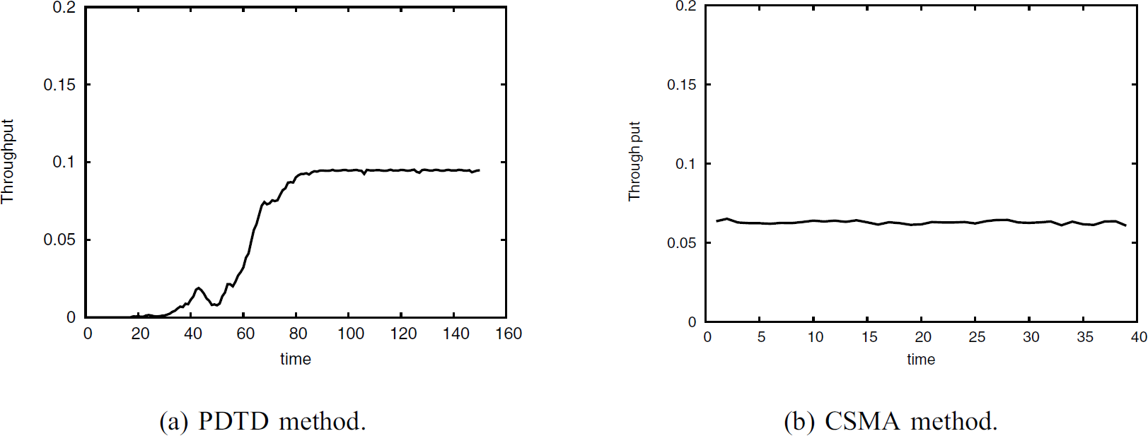
Comparison of average throughput.

FIGURE 17

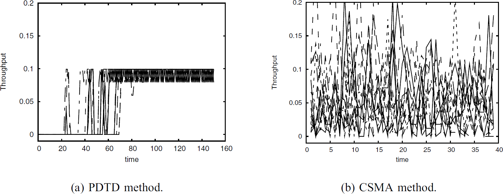
Comparison of throughput of nodes in 2hop neighborhood node 189.

FIGURE 18

Comparison of frequency of communication.

TABLE 2

Throughput value around center corresponding to Fig. 18

Node ID	149	168	169	170	187	188	189	190	191	208	209	210	229
PDTD	0.094	0.095	0.094	0.094	0.094	0.094	0.094	0.094	0.094	0.094	0.094	0.094	0.094
CSMA	0.044	0.036	0.064	0.066	0.049	0.056	0.054	0.078	0.074	0.053	0.066	0.054	0.052

C) Hardware Experiment

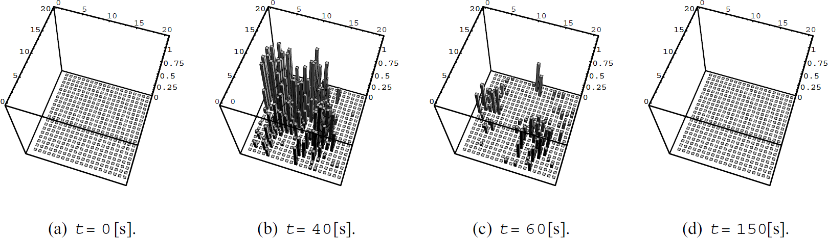
Preliminary hardware experiment is implemented to verify a basic functioning of the proposed method. The virtual node dynamics is installed on wireless sensor node devices, which features ZigBee protocols or IEEE 802.15.4 for WPAN (Wireless Personal Area Network). Figure 19 is a hardware experiment snapshot. In this system, the laptop computer monitors all of the pulse signals from the wireless devises, and displays the phase relation of them. The white circle in the screen shows the node under pulse transmission. This is a simplified case, so there are no hidden terminal nodes. Figure 19 (a) shows a case that the phase difference pattern comprised of 4 nodes is properly formed without communication collisions. With addition of the wireless devises to 8, collision occurs as shown in Figure 19 (b), where two phases are very close. Each node generates the virtual node according to the incremental pulse signals, then the phase dynamics modifies the phase difference distribution as shown in 19 (c) to avoid a collisional state. Meanwhile, if a device is removed (or turned off), a virtual node is deleted and the phase distribution is reformed as shown in 19 (d). Where, node id is not referred for the adaptation. From this result, the principle of the method is confirmed by the hardware experiment, but this experiment does not deal with a stochastic adaptation for which a large number of nodes must be provided and tested in a large fields.

FIGURE 19

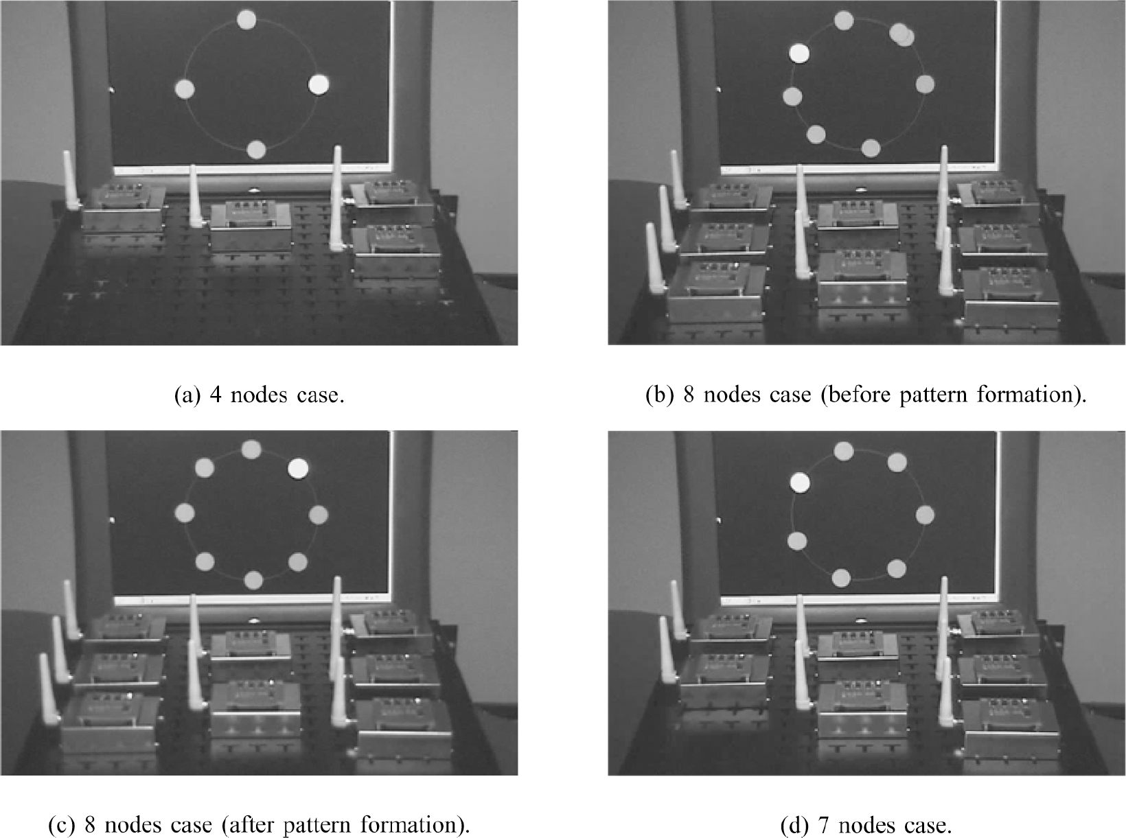
Hardware experiment.

5. Conclusion

In this paper we proposed a novel communication timing control method for the wireless sensor networks, named Phase Diffusion Time Division method. The PDTD method realizes a fully distributed and local information based timing control, which can be an alternative media access control to CSMA and the other related methods. The feature of PDTD is summarized as a self-organization of the phase difference division pattern through the coupled phase oscillatory dynamics with the stochastic adaptation. In addition to realization of the collision avoidance in a large scale network, assuring communication throughputs is also an important issue. Simulation experiments showed satisfactory results for a sufficiently large scale network for practical applications. However, it should be noted that we idealized the properties of wireless communication, where the communication range is represented as a circle. It may be asymmetrical according to the location in real fields because of influences from mobile objects. Therefore, it is required to discuss these aspects for more realistic and difficult situations. Also, hardware experiments are essential to reflect actual constraints and conditions to the theory. The virtual node dynamics is implemented to the wireless communication devises to verify basic functions to cope with addition and deletion of arbitrary nodes. A large scale experiment in the real fields is also on going work.