Sage Journals: Discover world-class research

Abstract

The original minimal exposure path problem in wireless sensor networks did not consider path constraint conditions. To consider the actual demand, this article proposes a minimal exposure path problem that requires the passage of the path through the boundary of a certain region. In this situation, because a corresponding weighted graph model cannot be developed, the methods that are used to solve the original minimal exposure path problem (the grid method and the Voronoi diagram method) are ineffective. Thus, this article first converts the problem into an optimization problem with constraint conditions. Because of the difficulty in finding a solution due to the model’s high nonlinearity and high dimensional complexity, as well as the special characteristics of the problem, a hybrid genetic algorithm is proposed to find the solutions. This article also provides a proof for the convergence of the designed algorithm. A series of simulation experiments demonstrates that the designed optimization model with constraints and the hybrid genetic algorithm can effectively solve the proposed minimal exposure path problem.

Keywords

Wireless sensor networks minimal exposure path hybrid genetic algorithm constraint condition

Introduction

Wireless sensor networks (WSNs) are composed of large numbers of sensor nodes that have sensing, data processing, and wireless communication functionalities. Because of their advantages of low cost and expendability, WSNs have been widely used in commercial and military fields (e.g. environmental monitoring, earthquake and weather forecasts, underground and deep-water probes). Research and applications of WSNs have attracted the attention of many researchers and manufacturers.

Coverage is one of the key fundamental technologies of WSNs; it reflects the WSN’s perceptibility of the monitored region. The coverage quality directly influences the performance of the monitoring system, and the measurement of coverage quality helps to describe the coverage of the entire network for the monitored targets (stationary or moving targets); it is also helpful in guiding the adjustment and optimization of sensor node deployments.

There have been many discussions about measuring coverage for target detection,^1–7 and most have concentrated on fence coverage problems. From the perspective of the characteristics of the monitored objects,¹ the coverage problem in WSNs can be categorized into regional coverage, scanning coverage, and fence coverage. The goal of research on fence coverage is to find one or multiple paths that connect the starting point to the end point, so these paths can describe the quality of detection and monitoring of moving targets under different definitions of coverage quality. “Exposure crossing”^2,8 simultaneously considers the temporal factor of “target exposure” and the special factor of the “sensing strength” of the sensor node on the target. Mathematically, it can be described as the integration of the sensing strength curve along the crossing path over time and space, and it is used to judge the quality of the coverage of a deployed sensor node on the exposure path. This measuring method was first discussed for the fence coverage problem and is currently the most widely used method.^2,8 The path that corresponds to the minimal exposure crossing is called the minimal exposure path; the problem of searching for this path is called the minimal exposure path problem.

It is pretty remarkable that in the practical WSN coverage problems, the importance of each location in the covered region might not be the same; for example, some regions in the area might be more sensitive. In addition, due to particular conditions (such as high temperatures, harsh environments, or sensitive and dangerous regions), some regions are not accessible; sensor nodes cannot be deployed within these regions, and the only option to protect these regions is to deploy sensors in the surrounding area. The moving target starts at a fixed point. When it reaches a sensitive region, it can only move along the boundary of the region (a small portion of the path in Figure 1 belongs to the boundary of this sensitive region) and then reaches the fixed end point. Thus, the ability of the WSN to monitor the moving target from the starting point to the end point along a certain path needs to be quantified, and the path with minimal exposure must be obtained. For convenience, this type of sensitive region is called a special protection region and corresponds to the problem discussed in previous studies.^2,8 The path that is sought is called the minimum exposure path problem with constraint conditions (MEP-CC problem). The proposed MEP-CC problem in this article considered that the mobile target only can move along some part border of a special region as it cannot get through this special region. There is no restriction that the region is whether in the middle of the monitoring area.

Figure 1.

A minimal exposure problem that contains special protection region boundary condition constraints.

The main contributions of this article are as follows:

To consider realistic scenarios, this article proposes a minimal exposure path problem with constraint conditions. The problem considers the special requirement that the moving target can only move along the boundary of an inaccessible area of the covered area because sensors cannot be deployed in that region.

In contrast to the traditionally used grid-based method and Voronoi-diagram-based method, this article first abstracts the proposed MEP-CC problem into an optimization model with constraints, which allows the use of mathematical optimization methods to solve the MEP problem.

Due to the difficulty in solving the designed complex high dimensionality and highly nonlinear optimization model with constraint conditions, this article considers the characteristics of the actual problem and designs a reasonable form of the fitness function and a local searching method that can eliminate paths with sawtooth patterns. A hybrid genetic algorithm is designed to solve the proposed MEP-CC problem, and the proof of the overall convergence of the algorithm is provided.

The MEP-CC problem proposed in this article is an expansion of the original MEP problem; the designed solution method is suitable for large-scale sensor node deployments.

The remaining content and structure of this article are as follows: In section “Related works,” we present some related works in MEP problem. Section “Problem description” introduces the basic concepts and limitations of the traditional MEP problem and proposes a MEP-CC problem that contains a special protection region. Section “Multivariate optimization model for the minimal exposure path problem with special protection region boundary condition constraints” analyses the reason that traditional MEP problem-solving methods are ineffective for the proposed problem and then develops a multi-variant optimization model. Section “A hybrid genetic algorithm” analyses the highly nonlinear characteristics of the new model, combines the characteristics of the practical problem, and designs a hybrid genetic algorithm. Section “Global convergence analysis of the hybrid genetic algorithm” provides a proof for the convergence of the designed algorithm. Section “Experiments and discussions” develops and analyses six experimental scenarios (including deterministic, random, and large-scale deployments of sensor nodes), and section “Conclusion” presents the conclusions.

Related works

The essence of the minimal exposure path (MEP) problem is the curve extreme problem in mathematics,⁹ which is also called the functional extreme variational problem.¹⁰ A common mathematical method of solving the variational problem is to solve the corresponding Euler–Lagrange differential equation;⁵ an analytical solution of this differential equation can provide a precise expression of this path. However, in the multiple sensor nodes scenario, the Euler–Lagrange differential equation is difficult to express and is even more difficult to solve due to its high nonlinearity. Thus, an accurate analytical solution cannot be obtained even when the mathematical essence of this problem had been determined.^11–13 Currently, the only available accurate analytical solution is for a single sensor node scenario;¹¹ only approximation solutions are available for the minimal exposure path problem in the multiple sensor nodes scenario. Approximation solution methods mainly include grid-based searching methods and the Voronoi-diagram-based computational geometric method. Meguerdichian et al.¹⁴ first designed an exposure crossing problem-solving method based on the idea of grids. This method first divides the sensing region into square grids, calculates the degree of exposure of each side of the grid based on the node distribution, and uses a shortest path algorithm, such as the Dijkstra algorithm, to find the path that crosses the sensing region and has the minimum exposure. The Voronoi-diagram-based computational geometric method was proposed by Veltri et al.¹⁵ The set of next candidate positions of the moving target is analyzed through a Voronoi diagram; at the same time, the degree of exposure of the moving object that follows the path during a certain time period is defined as the sensing strength of the sensor nodes along the path. Improvements to these two methods and applications to various scenarios have been proposed: several studies^11,12 have combined the Voronoi diagram method with the Euler–Lagrange differential equation for a single sensor node and have proposed an improved method, while another study¹³ applied the grid method to solve for the minimal exposure path of anisotropic sensor nodes. These studies address variants and applications of the grid method and the Voronoi diagram method for specific situations.

The mathematical problem that corresponds to the MEP-CC problem is the curve extreme fitting problem,⁹ and the essence is a variational problem (unilateral variational problem with functional extremes).^9,10 Similar to the original MEP problem, under the multiple sensor nodes scenario, the MEP-CC problem cannot be solved by solving Euler–Lagrange partial differential equations. Due to the constraints of the protected region boundary conditions, a corresponding weighted diagram model cannot be developed; the two basic types of approximation solution methods, the grid-based method and the Voronoi-diagram-based method, are also no longer appropriate. To solve this type of problem, this article first abstracts the MEP-CC problem with a special protection region into an optimization problem with constraints. This optimization problem is a complex problem of high dimensionality and high nonlinearity; it is difficult for traditional mathematical optimization methods to find an overall optimized solution. Under the framework of a genetic algorithm, this article combines the characteristics of the problem and designs a hybrid genetic algorithm solution method. A series of experiments demonstrates that the designed model and solution method can solve this new minimal exposure path problem. Compared with the grid-based and Voronoi-diagram-based methods, the designed method can not only be applied to the MEP-CC problem but also to the original MEP problem and is more general than the existing method.

Problem description

Degree of exposure and the minimal exposure path problem

The degree of exposure was first defined by Meguerdichian and colleagues.^2,8 Assume that m sensors, s₁, s₂, …, s_m, are distributed within the range of sensing region A to monitor a moving target crossing A. These sensor nodes can capture their own position information through some defined mechanism^16–18 and can ensure the reliability of coverage of the areas surrounding them.^19–21 A moving target travels from a fixed starting point s along a path P across region A to a fixed end point. The mathematical definition of the degree of exposure is^2,8

E (P, s, d) = \int_{P} I (p) dp

(1)

where I(P) represents the sensing strength of m sensors, s₁, s₂, …, s_m, when detecting the moving target at a certain point p on path P. Common expressions of I(P) include the full sensing mode $I (p) = \sum_{i = 1}^{m} I_{s_{i}} (p)$ and the maximum sensing value sensing mode $I (p) = \max_{i = 1, \dots, m} (I_{s_{i}} (p))$ , where $I_{s_{i}} (p)$ represents the sensing value of sensor node s_i when detecting a target at position p.^2,8,14 The sensing value of a commonly seen single sensor node s_i is $I_{s_{i}} (p) = λ / [d (s_{i}, p)]^{μ}$ , where λ and µ are device-related constants^2,8 and $d (s_{i}, p)$ represents the Euclidean distance between s_i and p. For convenience, in subsequent discussions, I(P) is the mode with the maximum sensing value; however, the designed method is not limited to this mode.

The MEP problem (for convenience, this is called the original MEP problem in the remainder of this article) is to find the path that connects the starting point s to the end point d that has the minimum degree of exposure. Assuming that path P can be expressed in the form y = y(x), equation (1) is a function of the function y(x), and it can be described mathematically as a functional^11–13

\begin{array}{l} J_{1} (y) = E (P, s, d) = \int_{P} I (p) d p \\ = \int_{y = y (x)} I (x, y) d s = \int_{y = y (x)} I (x, y) \sqrt{1 + {y^{'}}^{2}} d x \end{array}

The MEP problem can thus be expressed as

y^{*} = \underset{y}{\arg \min} J_{1} (y) = \underset{y}{\arg \min} \int_{y = y (x)} I (x, y) \sqrt{1 + {y'}^{2}} dx

(2)

A minimal exposure path problem with constraint conditions

In practical field applications, certain regions within the sensing region A need to be protected. However, limitations that are caused by some conditions, such as geospatial restrictions; harsh environments; or unreachable, dangerous, and sensitive regions, prevent sensor nodes from being deployed in some locations, and the only option is to pre-deploy sensor nodes around these regions. The moving target cannot enter this region; when it approaches the region from the starting point, it can only move along the boundary of the region. It will then leave the boundary at a certain point and eventually reach the end point. In the example shown in Figure 1, the region within the curve f(x, y) = 0 is a sensitive region that needs to be protected. Due to the local conditions, sensor nodes cannot be deployed within the region f(x, y) < 0 and can only be deployed in the region f(x, y) > 0. The moving target departs from the starting point s, follows a path, reaches point c on the boundary of the protected region, moves along the boundary to point k, and then follows a path from k to point d. The goal is to find the path with the minimal degree of exposure. This is the MEP problem with a special protected region boundary constraint condition, which corresponds to the curve extreme fitting problem in mathematics⁹ (unilateral variational problems with functional extremes).^9,10

The path in Figure 1 can be expressed as being composed of three path segments, $\overset{⌢}{sc}$ , $\overset{⌢}{cnk}$ , and $\overset{⌢}{kd}$ . By letting the set of $\overset{⌢}{cnk}$ points on the curve be $C_{f} = {〈 x, y 〉 | y = f (x)}$ , the degree of exposure can then be expressed as

\begin{array}{l} J_{2} (y) = \int_{\overset{⌢}{s c}} I (x, y) \sqrt{1 + {y^{'}}^{2}} d x + \int_{\overset{⌢}{c n k}} I (x, y) \sqrt{1 + {y^{'}}^{2}} d x \\ + \int_{\overset{⌢}{k d}} I (x, y) \sqrt{1 + {y^{'}}^{2}} d x \end{array}

The MEP problem that contains a must-pass region boundary can then be expressed as

\begin{matrix} y^{*} = \underset{y}{\arg \min} J_{2} (y) \\ s . t . \overset{⌢}{cnk} \subseteq Cf \end{matrix}

(3)

The constraint condition represents that the integration path $\overset{⌢}{cnk}$ is part of the curve f = f(x, y). This proposed MEP-CC problem considers the actual conditions, including the requirement that the moving target can only move along a portion of the boundary because sensors cannot be deployed in part of the covered area due to inaccessibility.

Multivariate optimization model for the minimal exposure path problem with special protection region boundary condition constraints

The common solution methods for the original MEP problem^2,8 include the grid-based method¹⁴ and the Voronoi-diagram-based method;¹⁵ both methods abstract the problem into a diagram model to obtain the solution. However, the grid method is ineffective for the minimal exposure path problem with a must-pass region boundary constraint proposed in this article because the constraint condition makes it impossible to calculate the weight of the grid node that corresponds to the boundary position of the constraint region; thus, the corresponding weighted diagram model cannot be developed. The Voronoi diagram method is also ineffective for the proposed problem because the constraint condition destroys the connection between the boundary of the protected region and the Voronoi vertex, so the corresponding weighted diagram model cannot be developed. As discussed in section “Introduction,” the core of the MEP-CC problem with a special protection region boundary (3) is a functional extreme with constraints problem, and the variational method cannot be used to obtain accurate analytical solutions of functional extreme problems.^11–13

Based on these considerations and analysis, this article employs an indirect functional extreme solving method: the finite difference method.¹⁰Figure 2 illustrates the path $\overset{⌢}{scnkd}$ from Figure 1 after being discretized by the finite difference method. The region $[x_{s}, x_{d}]$ is divided into n equal segments; the series of coordinate points $y_{0}, y_{1}, \dots, y_{n - 1}$ that correspond to $x_{0}, x_{1}, \dots, x_{n - 1}$ , $〈 x_{0}, y_{0} 〉, 〈 x_{1}, y_{1} 〉, \dots, 〈 x_{n - 1}, y_{n - 1} 〉$ can be used to approximate the path $\overset{⌢}{scnkd}$ . For convenience, let $F (x, y, y') = I (x, y) \sqrt{1 + {y'}^{2}}$ ; then, $J_{2} (y)$ can be expressed as

\begin{matrix} J_{2} (y) & = \int_{\overset{⌢}{sc}} I (x, y) \sqrt{1 + {y'}^{2}} dx + \int_{\overset{⌢}{cnk}} I (x, y) \sqrt{1 + {y'}^{2}} dx \\ + \int_{\overset{⌢}{kd}} I (x, y) \sqrt{1 + {y'}^{2}} dx \\ = \int_{x_{0}}^{x_{c}} F (x, y, y') dx + \int_{x_{c}}^{x_{k}} F (x, y, y') dx \int_{x_{k}}^{x_{d}} F (x, y, y') dx \\ \approx \sum_{i = 0}^{n - 1} F (x_{i}, y_{i}, \frac{Δ y_{i}}{Δ x_{i}}) Δ x \\ = \sum_{i = 0}^{p - 1} F (x_{i}, y_{i}, \frac{Δ y_{i}}{Δ x_{i}}) Δ x + \sum_{p}^{q - 1} F (x_{i}, y_{i}, \frac{Δ y_{i}}{Δ x_{i}}) Δ x \\ + \sum_{q}^{n - 1} F (x_{i}, y_{i}, \frac{Δ y_{i}}{Δ x_{i}}) Δ x \end{matrix}

(4)

where $x_{i}, i = 0, \dots, n - 1$ are pre-determinable constants, $x_{0} = x_{s}$ , $x_{n} = x_{d} = x_{0} + n Δ x$ , $y_{0} = y (x_{s}) = y_{s}$ , $y_{n} = y (x_{d}) = y_{d}$ , $x_{p} = x_{0} + (p - 1) Δ x$ , $x_{q} = x_{0} + (q - 1) Δ x$ , and p and q are integers that satisfy $x_{p - 1} \leq x_{c} \leq x_{p}$ and $x_{q - 1} \leq x_{c} \leq x_{q}$ , respectively.

Figure 2.

A path that has been discretized by the finite difference method.

The constraint condition $\overset{⌢}{cnk} \subseteq Cf$ can be stated as follows: when $p \leq j \leq q$ , $y_{j} = f (x_{j})$ . The variables to be determined in equation (4) are p, q, and $y_{i}, i = 0, \dots, n - 1$ . By inserting constraint conditions, the MEP problem expressed in equation (3) can be expressed as the following multi-variant optimization problem with constraint conditions

\begin{matrix} (p^{*}, q^{*}, y_{1}^{*}, y_{2}^{*}, \dots, y_{n - 1}^{*}) = \underset{p, q, y_{1}, y_{2}, \dots, y_{n - 1}}{\arg \min} \\ (\begin{matrix} \sum_{i = 0}^{p - 1} F (x_{i}, y_{i}, \frac{Δ y_{i}}{Δ x_{i}}) Δ x + \sum_{p}^{q - 1} F (x_{i}, y_{i}, \frac{Δ y_{i}}{Δ x_{i}}) Δ x \\ + \sum_{q}^{n - 1} F (x_{i}, y_{i}, \frac{Δ y_{i}}{Δ x_{i}}) Δ x) + \sum_{p}^{q - 1} F (x_{i}, y_{i}, \frac{Δ y_{i}}{Δ x_{i}}) Δ x + \sum_{q}^{n - 1} F (x_{i}, y_{i}, \frac{Δ y_{i}}{Δ x_{i}}) Δ x \end{matrix}) \\ s . t . \forall p \leq j \leq q, y_{j} = f (x_{j}) \end{matrix}

(5)

A hybrid genetic algorithm

Many mathematical deterministic optimization methods can be used to find solutions to optimization problems, such as the steepest descent method,²² the quasi-Newton method,²³ and the filled function method.²⁴ However, these methods require information such as the derivative of the function and can only be used in global optimization problems with well-behaved functions; they are difficult to use for complex engineering optimization problems. The form of the derivative of the optimization object function $\sum_{i = 0}^{n - 1} F (x_{i}, y_{i}, (y_{i + 1} - y_{i}) / Δ x) Δ x$ in equation (5) is very complex, and the dimensionality of the continuous variable $y_{1}, y_{2}, \dots, y_{n - 1}$ is quite high; thus, classical deterministic optimization methods are not suitable for solving this optimization problem.

Compared to the deterministic optimization methods described above, stochastic optimization methods have fewer requirements for the functions; only the values of the functions are needed, and there are few requirements for the properties of the objective functions (e.g. differentiability, continuity). They can be used to solve most optimization problems and are well suited for complex engineering optimization problems. This article uses the genetic algorithm,²⁵ which is a relatively mature stochastic optimization method, to design a method to solve the MEP-CC problem. However, the direct application of the standard genetic algorithm would result in a sawtooth-shaped path (Figure 3) because of the difficulty in controlling the amount of computation of the genetic algorithm when solving high-dimensional nonlinear optimization problems; thus, the rate of convergence toward the global optimized solution is slow. Many researchers^26–32 have studied the fundamental theory and techniques of the genetic algorithm in detail and have designed operators to speed up the convergence and improve the quality of the optimized solutions as well as the corresponding hybrid genetic algorithms. This article designed a key fitness function and a highly efficient local search method by considering the actual problem, which can effectively eliminate the occurrence of the sawtooth path solution and increase the convergence speed. The specific analysis and design process is as follows.

Figure 3.

Part of a path that corresponds to the continuous component $(y_{i}, y_{i + 1}, y_{i + 2}, \dots, y_{i + k})$ . The dashed line represents the sawtooth-shaped path obtained by connecting the point sequence $〈 x_{i}, y_{i} 〉, 〈 x_{i + 1}, y_{i + 1} 〉, 〈 x_{i + 2}, y_{i + 2} 〉, \dots, 〈 x_{i + k}, y_{i + k} 〉$ ; the solid line represents the curve $y^{*} = g (x)$ after curve fitting the point sequence.

Fitness function

Only a well-designed fitness function can guide the algorithm in a desired searching direction. The genetic algorithm is an iterative searching algorithm; thus, designing a fitness function with a good form is critical. In the optimization problem equation (5), the continuous variable to be optimized is $Y = [y_{1}, y_{2}, \dots, y_{n - 1}]$ , which has a dimensionality of n − 1. If the calculated values of the degree of exposure in equation (4) are used directly as the fitness function, for convenience, let $φ (y_{1}, y_{2}, \dots, y_{n - 1}) = \sum_{i = 0}^{n - 1} F (x_{i}, y_{i}, (Δ y_{i} / Δ x_{i}) Δ x = \sum_{i = 0}^{n - 1} F (x_{i}, y_{i}, ((y_{i + 1} - y_{i}) / Δ x) Δ x = \sum_{i = 0}^{n - 1} I (x_{i}, y_{i}) \sqrt{1 + {((y_{i + 1} - y_{i}) / Δ x)}^{2}} Δ x$ . The degree of path jumping cannot be accurately reflected; the sensing strength value $I (x, y)$ changes dramatically in segments that contain large jumps, which will lead to significant calculation errors. If we let $d_{i} = \sqrt{{(x_{i + 1} - x_{i})}^{2} + {(y_{i + 1} - y_{i})}^{2}}$ express the distance between points $〈 x_{i}, y_{i} 〉$ and $〈 x_{i + 1}, y_{i + 1} 〉$ , then $\max_{i} (d_{i}), i = 1, \dots, n - 1$ can reflect the degree of sawtooth jumping of the path; the smaller the value, the better the result. The ideal situation is to hope that the change in the sensing strength value $I (x, y)$ is as small as possible on every line segment and that the minimum amount of jumping occurs. By considering both of these factors, this article changed the fitness function to $φ (y_{1}, y_{2}, \dots, y_{n - 1}) = \sum_{i = 0}^{n - 1} (\max_{p \in (〈 x_{i}, y_{i} 〉, 〈 x_{i + 1}, y_{i + 1} 〉)} I (p)) d_{i} + \max_{i} (d_{i}) \sum_{i = 0}^{n - 1} d_{i}$ , where the first sum replaces the original $I (x, y)$ value by the upper limit of the sensing strength value $\max (I (x, y))$ in that line segment, which represents the penalty for the first factor, and the second sum represents the penalty for the second factor; the bigger the sawtooth jump, the larger the value of $\max_{i} (d_{i})$ and the larger the value after being multiplied by the path length $\sum_{i = 0}^{n - 1} d_{i}$ . This design is based on the idea of penalty functions but reduces the discussion of penalty parameters compared to the common penalty function method. It also considers the degree of approximation of the degree of exposure as well as the way to reduce the occurrence of sawtooth jumping, and it can help an individual population member evolve in a good direction.

Coding and constraint condition treatment

The variables to be optimized in the optimization problem (5) include the n − 1dimensional continuous variables $y_{1}, y_{2}, \dots, y_{n - 1}$ . Based on the analysis presented above, the constraint condition $\overset{⌢}{cnk} \subseteq Cf$ can be stated as follows: when $p \leq j \leq q$ , $f (x_{j}, y_{j}) = 0$ must be satisfied. Thus, the variables to be optimized include the integers p and q in addition to $y_{1}, y_{2}, \dots, y_{n - 1}$ . Hybrid coding can be used to treat these variables, $C = [p, q, y_{1}, y_{2}, \dots, y_{n - 1}]$ , in which p and q are integers between 1 and n − 1 and $p \leq q$ . The allowed range of the continuous variables $y_{1}, y_{2}, \dots, y_{n - 1}$ can be expressed as follows: when $p \leq j \leq q$ , $y_{j} = f (x_{j})$ ; other values of $y_{j}$ are in the sensing region A.

Population initialization

Following the normal method, the individual population members $C = [p, q, y_{1}, y_{2}, \dots, y_{n - 1}]$ are initialized randomly

\begin{matrix} p = rand int (c, k); \\ q = rand int (c, k); \\ Y_{i, j} = {\begin{matrix} Y_{\min, j} + rand (0, 1) (Y_{\max, j} - Y_{\min, j}) & if j < c or j > k \\ f (x_{j}) & if c \leq j \leq k \end{matrix} \end{matrix}

(6)

where $rand int (c, k)$ represents a random integer between c and k, and c and k represent integers that correspond to the upper limit $x_{left}$ and lower limit $x_{right}$ , respectively, of the horizontal components of the boundary.

Crossover operator

For two different individual members $C_{a} = [p_{a}, q_{a}, y_{a, 1}, y_{a, 2}, \dots, y_{a, n - 1}]$ and $C_{b} = [p_{b}, q_{b}, y_{b, 1}, y_{b, 2}, \dots, y_{b, n - 1}]$ , consider using the convex combination method to search for a new member. If the newly generated member is represented by $C_{v} = [p_{v}, q_{v}, y_{v, 1}, y_{v, 2}, \dots, y_{v, n - 1}]$ , then the searching equation is

{\begin{matrix} p_{v} = int (λ p_{a} + (1 - λ) p_{b}) \\ q_{v} = int (λ q_{a} + (1 - λ) q_{b}) \\ y_{v, i} = f (x_{i}), if p_{v} \leq i \leq q_{v}, \\ y_{v, i} = y_{a, i} + φ_{a, b} (y_{b, i} - y_{a, i}), if i \leq p_{v} or i \geq q_{v} \\ i = 1, \dots, n \end{matrix}

(7)

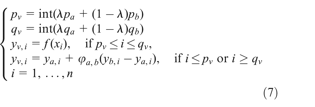
where int represents a rounding function, $λ$ is a random number between 0 and 1, and $φ_{a, b}$ is a random number within [−1, 1].

To ensure that the individual is legitimate, for the $y_{v, i}$ component outside the allowed range, take the nearest boundary value. The design of equation (7) ensures that the algorithm has the ability to conduct a global search.

Mutation

Multiple Gaussian mutations are used; every component of the continuous variable $Y = (y_{1}, y_{2}, \dots, y_{n - 1})$ of the individual $C = [p, q, y_{1}, y_{2}, \dots, y_{n - 1}]$ is Gaussian perturbed to obtain a new individual $Y^{m}$ ; that is, $Y^{m} = Y + η$ , where $i \leq p$ or $i \geq q$ , $η = (η_{1}, η_{2}, \dots, η_{n - 1})$ , $η_{i} ~ N (0, σ^{2}), i = 1, \dots, n - 1$ , $N (0, σ^{2})$ represents a Gaussian distribution with a mean of zero and a variance $σ^{2}$ , and each component $(η_{1}, η_{2}, \dots, η_{n - 1})$ is independent. The integral component $N = [p, q]$ of $C = [p, q, y_{1}, y_{2}, \dots, y_{n - 1}]$ only needs Gaussian mutation to obtain $N_{m} = [p_{m}, q_{m}]$ , where $p^{m} = p + η_{p}$ , $η_{p}$ is an integer that is obtained by rounding a zero mean Gaussian distribution with a variance of $σ^{2}$ , and $η_{p} = int (N (0, σ_{p}^{2}))$ ; the same process is used for $q^{m} = q + η_{q}$ , $η_{q} = int (N (0, σ_{q}^{2}))$ . The mutated individual is

C_{m} = [N_{m}, Y_{m}] = [p + η_{p}, q + η_{q}, Y + η]

(8)

where $η$ is an independently distributed multiple-dimension Gaussian distribution function.

Local search operator

For the integral component and continuous component contained in the individual $C = [p, q, y_{1}, y_{2}, \dots, y_{n - 1}]$ , corresponding local search methods must be designed separately.

Local search for the continuous component

Because equation (5) is a highly nonlinear and high-dimensional optimization problem, the convergence rate is not sufficiently fast when the standard genetic algorithm is used, and a solution with a sawtooth-shaped curve is often obtained (Figure 3). For a high dimensionality and highly nonlinear complex fitness value function $φ (y_{1}, y_{2}, \dots, y_{n - 1}) = \sum_{i = 0}^{n - 1} (\max_{p \in (< x_{i}, y_{i} >, < x_{i + 1}, y_{i + 1} >)} I (p)) d_{i} + \max_{t} (d_{i}) \sum_{i = 0}^{n - 1} d_{i}$ , when dealing with the continuous component $y_{i}$ , and $j \leq p$ or $j \geq q$ , we consider obtaining the local extreme value of these continuous components $y_{i}$ , $y_{i}^{*}$ . Due to the existence of penalty operators, designing a practical local search operator is very difficult. Thus, one can avoid analyzing the complex function form $φ (y_{1}, y_{2}, \dots, y_{n - 1})$ and instead consider a simple function form $\sum_{i = 0}^{n - 1} I (x_{i}, y_{i}) \sqrt{Δ x^{2} + {(y_{i + 1} - y_{i})}^{2}}$ . The local search operator for the continuous component $y_{i}$ is designed as follows.

A gene segment $(y_{i}, y_{i + 1}, y_{i + 2}, \dots, y_{i + k})$ of the continuous component $Y = (y_{1}, y_{2}, \dots, y_{n - 1})$ is locally optimized; the goal is to hope that the value of the gene segment $({\bar{y}}_{i}, {\bar{y}}_{i + 1}, {\bar{y}}_{i + 2}, \dots, {\bar{y}}_{i + k})$ after the optimization not only reduces the sawtooth pattern in Figure 3 but also minimizes the value of the function $\sum_{i = 0}^{n - 1} I (x_{i}, y_{i}) \sqrt{Δ x^{2} + {(y_{i + 1} - y_{i})}^{2}}$ , which achieves the effect of the local search. For this, we first consider performing a curve fitting (such as polynomial fitting) for the coordinate points $〈 x_{i}, y_{i} 〉, 〈 x_{i + 1}, y_{i + 1} 〉, 〈 x_{i + 2}, y_{i + 2} 〉, \dots, 〈 x_{i + k}, y_{i + k} 〉$ , which are represented by $(y_{i}, y_{i + 1}, y_{i + 2}, \dots, y_{i + k})$ . Let the fitted function be represented by $y^{*} = g (x)$ , as shown by the solid line in Figure 3; thus, the significant sawtooth pattern can be eliminated. Second, we consider designing a local optimization method that would decrease the value of $\sum_{i = i}^{i + k} I (x_{i}, y_{i}) \sqrt{Δ x^{2} + {(y_{i + 1} - y_{i})}^{2}}$ . Because the fitted function obtained previously can reduce the distance between two adjacent points $\sqrt{Δ x^{2} + {(y_{i + 1} - y_{i})}^{2}}$ , it is only necessary for the sensing strength $I (x_{i}, y_{i})$ to take the local minimum to decrease the overall value of the product $I (x_{i}, y_{i}) \sqrt{Δ x^{2} + {(y_{i + 1} - y_{i})}^{2}}$ and thus obtain a local optimization. For this, the value of the fitted function $(y_{i}^{*}, y_{i + 2}^{*}, y_{i + 2}^{*}, \dots, y_{i + k}^{*})$ will be within a range of $(y_{i}^{*}, y_{i + 2}^{*}, y_{i + 2}^{*}, \dots, y_{i + k}^{*})$ so that the corresponding $I (x, y)$ is minimized; that is

\begin{matrix} {\bar{y}}_{i + j} = \underset{y_{i + j} \in [y_{i + j}^{*} + Δ, y_{i + j}^{*} - Δ]}{\arg \min} I (x_{i + j}, y_{i + j}) \\ j = i, i + 1, i + 2, \dots, i + k \end{matrix}

(9)

where $Δ$ is a predetermined constant, which is used to limit the search range of $I (x_{i}, y_{i})$ .

The gene segment value $({\bar{y}}_{i}, {\bar{y}}_{i + 1}, {\bar{y}}_{i + 2}, \dots, {\bar{y}}_{i + k})$ obtained in this manner can guarantee that $I (x_{i}, y_{i}) \sqrt{Δ x^{2} + {(y_{i + 1} - y_{i})}^{2}}$ , $I (x_{i + 1}, y_{i + 1}) \sqrt{Δ x^{2} + {(y_{i + 2} - y_{i + 1})}^{2}} \dots$ , $I (x_{i + k}, y_{i + k}) \sqrt{Δ x^{2} + {(y_{i + k + 1} - y_{i + k})}^{2}}$ are minimized for each k, which will make the sum $\sum_{j = i}^{i + k} I (x_{j}, y_{j}) \sqrt{Δ x^{2} + {(y_{j + 1} - y_{j})}^{2}}$ have a local minimum value and achieve the local search effect for the $k + 1$ dimensional components $y_{i}, y_{i + 1}, \dots, y_{i + k}$ .

Local search for the integral component

For the integral component $N = [p, q]$ of the individual $C = [p, q, y_{1}, y_{2}, \dots, y_{n - 1}]$ , the corresponding points $〈 x_{p}, y_{p} 〉$ and $〈 x_{q}, y_{q} 〉$ are both on the curve f = f(x), and the distance between two adjacent points $\sqrt{Δ x^{2} + {(y_{i + 1} - y_{i})}^{2}}$ can be determined by the curve f = f(x). Thus, we only need to search for the minimum value of the sensing strength $I (x, y)$ near $〈 x_{p}, y_{p} 〉$ and $〈 x_{q}, y_{q} 〉$ . The obtained integral component is represented by $\bar{N} = [\bar{p}, \bar{q}]$ ; thus, the local search for the integral component can be expressed as

\begin{matrix} \bar{p} = \underset{p \in [p - 1, p + 1]}{\arg \min} I (x_{p}, y_{p}) \\ \bar{q} = \underset{q \in [q - 1, q + 1]}{\arg \min} I (x_{q}, y_{q}) \end{matrix}

(10)

Selection method and production of the child population

In all of the individuals in the current population (parent generation) and all of the child populations (which are produced by crossovers and mutations), we select the first pop individuals to form the seed population for the next generation.

Hybrid genetic algorithm

Algorithm 1
Step 1 (Parameter initialization). Initialize the population size pop, the maximum number of generations GenMax, the crossover operator parameter $σ^{2}$ and the local search parameters k and $Δ$ .
Step 2 (Population initialization). For each individual C in the population, use hybrid coding $C = [p, q, y_{1}, y_{2}, \dots, y_{n - 1}]$ , initialize pop individuals via equation (6) as the initial population P(0), use $φ (y_{1}, y_{2}, \dots, y_{n - 1}) = \sum_{i = 0}^{n - 1} (\max_{p \in (〈 x_{i}, y_{i} 〉, 〈 x_{i + 1}, y_{i + 1} 〉)} I (p)) d_{i} + \max_{i} (d_{i}) \sum_{i = 0}^{n - 1} d_{i}$ as the fitness function of the individual object to calculate the fitness value for each individual, and let the generation number t = 0.
Step 3 (Crossover operator). Randomly select two individuals from the current population P(t), produce two child individuals via equation (7), and repeat the crossover operation a certain number of times. All of the individuals from these crossover operations form a set, which is denoted as O₁.
Step 4 (Local search). For every individual $C = [p, q, y_{1}, y_{2}, \dots, y_{n - 1}]$ in O₁, use equation (9) to perform a local search for $k + 1$ components of the continuous component $Y = (y_{1}, y_{2}, \dots, y_{n - 1})$ after randomly selecting a location i. For the integral component $N = [p, q]$ , use equation (10) to perform a local search; the new individual set is denoted as O₂.
Step 5 (Mutation operator). Select the individuals in O₂ according to the probability p_m and use equation (8) to conduct the mutation operation. The new individual set is denoted as O₃.
Step 6 (Selection operation). Select the first pop individuals with the best fitness values from the set P(t)∪O₁∪O₂∪O₃ as the seed population for the next generation P(t + 1), and let t = t + 1.
Step 7 (Termination condition). Let t = t + 1. If the current generation number t is equal to the maximum number of generations GenMax, record the optimal seed population individuals and output them as the globally optimized approximation solution; if not, jump to Step 3 and continue the operations.

Global convergence analysis of the hybrid genetic algorithm

This section presents the mathematical analysis and proof of convergence for the designed algorithm. It is a kind of stochastic search iterative algorithm, during each iteration, the population is modified by a number of successive probabilistic transformations such as crossover operator, mutation operator, and designed local search operator. The resulting new population depends only on the state of the current population in a probabilistic manner. This property reveals that Algorithm 1 is of a stochastic nature. Notice that the deterministic concept of “convergence to the optimum” is not appropriate to define exact stochastic convergence as follows.

Let $X^{*} = {x^{*} \in S | f (x^{*}) = \min f (x), x \in S}$ denote the set of globally optimal solutions for the global optimization problem $\min_{x \in S} f (x)$ , where S represents the feasible region for x.

Definition 1

Let $x^{*} \in S$ denote one of the globally optimal solution for the global optimization problem $\min_{x \in S} f (x)$ . If

Prob {lim_{t \to \infty} x^{*} \in P (t)} = 1

then the proposed algorithm is called to converge to the global optimal solution with probability 1, where Prob{ } represents the probability of random event { }.

To discuss the globally convergent properties of the proposed Algorithm 1 , we need to introduce the following concepts.

Definition 2

For the given two chromosomes a and b, if

Prob {MC (a) = b} > 0

then b is called to be reachable from a by crossover and mutation, where MC(a) represents the offspring that were generated from chromosome a by crossover operator and mutation operator.

Bäck³³ and Rudolph³⁴ have proved the following Lemma 1.

Lemma 1

If a genetic algorithm with a finite search space S satisfies the following conditions, it will converge to the global optimal solution with probability 1 regardless of the initial population distribution.

Hypothesis 1. For any two chromosomes a, b ∈ S, b is reachable from a by crossover and mutation.

Hypothesis 2. The population sequence $P (0), P (1), \dots, P (k), \dots$ is monotone, that is, for ∀k

\min {f (x) | x \in P (k + 1)} \leq \min {f (x) | x \in P (k)}

For the proposed Algorithm 1 , the following conclusion applies.

Theorem 1

The proposed Hybrid Genetic Algorithm for the MEP-CC model (5) of the MEP problem converges to the global optimal solution with probability 1 regardless of the initial population distribution.

Proof of Theorem 1

According to the initial population generation method as described in section “Population initialization,” a solution $Y = (y_{1}, y_{2}, \dots, y_{n - 1})$ represents a path for the MEP problem, the feasible region is the vertical coordinates (denoted by $A_{y}$ ) of the sensing field F. Obviously, the object function in model (5) is a function in the feasible region with a certain lower bound; this demonstrates that the set of global optimal solutions is not empty.

First, it is proved that Algorithm 1 satisfies the Hypothesis 1,that is, for any two chromosomes $Y^{a} = (y_{1}^{a}, y_{2}^{a}, \dots, y_{n - 1}^{a})$ and $Y^{b} = (y_{1}^{b}, y_{2}^{b}, \dots, y_{n - 1}^{b})$ , $Y^{b}$ is reachable from $Y^{a}$ by crossover and mutation, in Steps 3, 4, and 5. Suppose that $Y^{c}$ is any offspring generated from a crossover in Step 3 and $Y^{d}$ is the individual generated from $Y^{c}$ by the proposed local search operation in Step 4. The probability of choosing $Y^{c}$ or $Y^{d}$ to take part in crossover is p_m > 0.

After applied local search operation in Step 4, if $Y^{d}$ is not improved, $Y^{c}$ should remain, then the probability of $Y^{b}$ being generated from $Y^{a}$ satisfies $Prob {MC (Y^{a}) = Y^{b}} = p_{m} • Prob {M (Y^{c}) = Y^{b}}$ , otherwise, replace $Y^{c}$ with $Y^{d}$ , then the probability of $Y^{b}$ being generated from $Y^{a}$ satisfies $Prob {MC (Y^{a}) = Y^{b}} = p_{m} • Prob {M (Y^{c}) = Y^{d} \in M_{ε}} • Prob {M (Y^{d}) = Y^{b}} = p_{m} • Prob {M (Y^{d}) = Y^{b}}$ .

Consider the probability of $Y^{b}$ being generated from $Y^{a}$ by mutation operator $Prob {M (Y^{c}) = Y^{b}}$ . According to the Gauss Mutation as described in section “Mutation,” every component is independent normal distribution, $y_{i}^{b} = y_{i}^{c} + η_{i}$ , then the probability density function of $η_{i}$ is $p (η_{i}) = (1 / \sqrt{2 π} σ) e^{- η_{i}^{2} / 2 σ^{2}}$ , and the probability density function of $η = (η_{1}, η_{2}, \dots, η_{n - 1})$ is $p (η) = 1 / (\sqrt{2 π} σ)^{n - 1} e^{- (η_{1}^{2} + η_{2}^{2} + \dots + η_{n - 1}^{2}) / 2 σ^{2}}$ ; we have $Prob {M (y^{c}) = y^{b}} = \int_{M_{F}} 1 / ({(\sqrt{2 π} σ)}^{n - 1}) e^{- (η_{1}^{2} + η_{2}^{2} + \dots + η_{n - 1}^{2}) / 2 σ^{2}} d η$ , where $M_{F}$ represents the feasible region corresponding to the plan F. For the bounded feasible region, there is a positive $θ > 0$ such that $η_{i}^{2} < θ$ . This conveys the conclusion $Prob {M (y^{c}) = y^{b}} \geq \int_{M_{F}} 1 / ({(\sqrt{2 π} σ)}^{n - 1}) e^{- (n - 1) θ / 2 σ^{2}} d η = 1 / (\sqrt{2 π} σ)^{n - 1} e^{- (n - 1) θ / 2 σ^{2}} m (M_{F}) > 0$ , where $m (M_{F})$ means the measure of the feasible region. So, we have $Prob {MC (Y^{a}) = Y^{b}} = p_{m} • Prob {M (Y^{c}) = Y^{b}} > 0$ . This proves that $Y^{b}$ is reachable from $Y^{a}$ .

The proof is similar for $Prob {MC (Y^{a}) = Y^{b}} = p_{m} • Prob {M (Y^{d}) = Y^{b}} > 0$ which also conveys the conclusion that $Y^{b}$ is reachable from $Y^{a}$ .

So, Algorithm 1 holds Hypothesis 1. Now, Algorithm 1 is proved to satisfy Hypothesis 2. In fact, it can be seen from the selection scheme at Step 6 of the proposed algorithm that P(k + 1) consists of the best pop chromosomes chosen from P(t)∪O₁∪O₂∪O₃ for t = 0, 1, … Thus, the population sequence P(0), P(1), …, P(t), … is proved to be monotone.

From Lemma 1, we have the conclusion Algorithm 1 that converges to the global optimal solution with probability 1 regardless of the initial population distribution.▪

Experiments and discussions

To test the effectiveness of the designed algorithm in solving the MEP-CC problem that contains protected regions, we designed a series of simulation experiments that include scenarios with deterministic and random distributions of sensor nodes outside the protected region.

The computer used as the test platform was configured with a 2.8 GHz Pentium(R) Dual-Core CPU E5500, 2 GB of RAM internal memory, and the Win XP (SP3) operating system. MATLAB 7.6.0 was used as the simulation software. Deterministic and random distributions (including the large-scale random node distribution) of the sensor nodes were established. The experimental parameters for the nodes were $λ = 4$ and $μ = 2$ . If not otherwise mentioned, the maximum sensing strength model was used. The parametric settings in the designed algorithm were a population size pop of 50 and a maximum number of generations GenMax between 150 and 300; if the number of nodes was less than 100, then GenMax was set to 150, and if the number of nodes was greater than 100, then GenMax was set to 300. The curve fitting results indicated that the average code size occupied by each sensor node should be at least 5. Thus, the code size dimension of the continuous component in the hybrid code $C = [p, q, y_{1}, y_{2}, \dots, y_{n - 1}]$ , codeSize, is set to the integer nearest to $5 (\sqrt{m} + 1)$ , where m is the number of sensor nodes. The value of k in the k-dimensional local search is critical. If the value is too small, then the effect of the multi-dimensional local search is very weak. When $k = 1$ , the search becomes a one-dimensional local search, which will affect the convergence speed; however, if the value is too large, then the algorithm can easily become trapped in local optima. Generally, a reasonable value for k is an integer between [codeSize/5] and [codeSize/6].

Scenario of the deterministic deployment of sensor nodes and experimental results

Experimental scenarios for the deterministic deployment of equilateral triangular and square sensor node distributions outside the protected region were designed; the specifics are as follows.

Scenario 1

The sensing region is a 10 m × 10 m square, and the bound of protected region is a parabola, which is marked by the solid blue line in Figure 4. In total, 31 sensor nodes are deployed deterministically outside the protected region, and no sensor nodes are deployed within the protected region. The adjacent sensor nodes outside the protected region form squares. The path starts at (0, 3.5) and ends at (10, 4.5); this scenario is shown in Figure 4(a) (the descriptions of these items in Figure 4 that shows the subsequent scenarios will not be repeated). The black stars mark the locations of the sensor nodes. The red plus signs and the red dashed line mark the minimal exposure path obtained; the number of every fifth point on the path is marked. The black dashed line marks the sides of the Voronoi diagram (usually called the Voronoi sides) that correspond to the sensor nodes; because the sensor nodes are distributed in squares, the corresponding Voronoi sides form a square grid. The values of the relevant parameters in the algorithm are as follows: the individual code size is 56, the population size is 50, and the local search parameters are Δ = 2 and k = 10. With the exception of the portion along the protected region boundary, the minimal exposure path outside the protected region almost always lies along Voronoi sides; this is consistent with the conclusions of traditional MEP problems.^1,14,15 The final fitness value is 57.2942. The curves in Figure 4(b) show the evolution of the optimum path during the 1st, 10th, 20th, 40th, 75th, and 150th generations of the seed populations.

Figure 4.

Scenario 1: starting point (0, 3.5); end point (10, 4.5); the special protection region is a parabola; and 31 sensors form a square distribution: (a) node deployment and final path result and (b) optimum path evolution process.

Scenario 2

In total, 30 sensor nodes are deployed deterministically in a 10 m × 10 m region; the adjacent sensor nodes outside the protected region are arranged in equilateral triangles. The path starts at (0, 3) and ends at (10, 5). The boundary of the protected region is a parabola, which is marked by the solid blue line in Figure 5, and no sensors were deployed within the protected region; this scenario is shown in Figure 5(a). Because the sensor nodes outside the protected region are deployed in equilateral triangles, the corresponding Voronoi diagram is a regular hexagonal grid. The values of the relevant parameters in the algorithm are as follows: the individual code size is 64, the population size is 50, and the local search parameters are Δ = 1.8516 and k = 10. As in the previous scenario, the minimal exposure path almost always follows Voronoi sides; this is consistent with the conclusions of traditional MEP problems.^1,14,15 The final fitness value is 95.3662. The curves in Figure 5(b) show the evolution of the optimum path during the 1st, 10th, 20th, 40th, 75th, and 150th generations of the seed populations.

Figure 5.

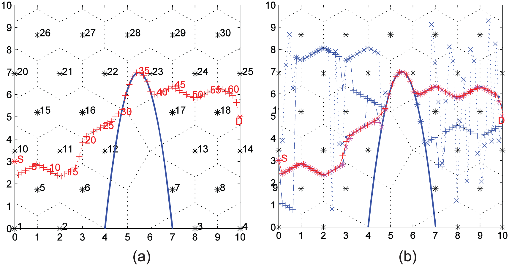
Scenario 2: starting point (0, 3); end point (10, 5); the special protection region is a parabola; and 30 sensors form a triangular distribution: (a) node deployment and final path result and (b) optimum path evolution process.

The minimal exposure paths outside the protected region follow Voronoi sides in both scenarios, which is consistent with the conclusions from previous studies.^1,14,15 This demonstrates the accuracy and reliability of this method of determining the minimal exposure path in scenarios with deterministic sensor node deployments.

Uniform random deployment of sensor nodes

To generate a uniform random deployment of sensor nodes, we produced coordinate locations for each sensor node $(x_{i}, y_{i})$ by generating uniform random numbers for the horizontal ( X ) and vertical ( Y ) components of a two-dimensional coordinate system. Four scenarios were generated.

Scenario 3 is in a 10 m × 10 m region, and the special protected region is a parabola marked by a solid blue line. A total of 46 sensor nodes are randomly deployed outside the protected region, and no sensors are located inside the protected region. This scenario is shown in Figure 6. Scenarios 4–6 use 160, 250, and 350 sensor nodes in a 100 m × 100 m region; these scenarios are shown in Figures 7 –9, respectively.

Figure 6.

Scenario 3: starting point (0, 40); end point (100, 50); 46 randomly distributed sensors; population size 50; codeSize = 72; total evolution generation 150; search range Δ = 16.9706, k = 8; and final fitness value 861.47: (a) node deployment and final path result and (b) optimum path evolution process.

Figure 7.

Scenario 4: starting point (0, 40); end point (100, 50); 160 randomly distributed sensors; population size 50; codeSize = 128; total evolution generation 150; search range Δ = 4.2, k = 10; and final fitness value 520.1987: (a) node deployment and final path result and (b) optimum path evolution process.

Figure 8.

Scenario 5: starting point (0, 40); end point (100, 50); 250 randomly distributed sensors; population size 50; codeSize = 152; total evolution generation 300; search range Δ = 6, k = 9; and final fitness value 1290.6453: (a) node deployment and final path result and (b) optimum path evolution process.

Figure 9.

Scenario 6: starting point (0, 40); end point (100, 50); 350 randomly distributed sensors; population size 50; codeSize = 176; total evolution generation 300; search range Δ = 5, k = 9; and final fitness value 758.4164: (a) node deployment and final path result and (b) optimum path evolution process.

The four scenarios with randomly deployed sensor nodes use increasing numbers of nodes and include situations with small- and large-scale random sensor node deployments; the corresponding dimensionality of the model (5) gradually increases as well. In Scenarios 4–6, the dimensionality of the continuous component exceeded 100; the dimensionality of the problem (individual code size) was very high. The algorithm can solve these problems very well. Outside the protected region, the obtained minimal exposure paths still follow Voronoi sides, which is consistent with the conclusions from previous studies.^1,14,15

Algorithm convergence speed

Due to space limitations, only the convergence performance of Scenario 4 is presented. The curves in Figure 10 represent the changing relationship between the optimal fitness value and the generation number that corresponds to Scenario 4. The curves decrease rapidly and converge to a stable state, which demonstrates that the designed algorithm rapidly converges to the global optimal solution and is highly efficient.

Figure 10.

Relationship between the optimal fitness value and evolution generation number. The horizontal axis is the generation number, and the vertical axis is the fitness value.

Conclusion

The original minimal exposure path problem considers a path from a fixed starting point to a fixed end point with no intermediate constraints. This article discusses the minimal exposure path problem with constraint conditions that arise from restrictions from the conditions (such as high temperatures, harsh environments, or sensitive or dangerous regions) that prevent the deployment of sensors in some inaccessible regions; thus, the sensor nodes can only be deployed in the areas surrounding these regions. The moving target departs from a fixed starting point, and when it encounters a sensitive region, it can only move along the boundary of the region. The target then reaches the fixed end point. The problem proposed and discussed in this article is a variant and extension of the original minimal exposure path problem. By considering the ineffectiveness of the original methods, this article abstracts the proposed problem into an optimization model. Despite the difficulty in solving the problem, which has a high model dimensionality and is highly nonlinear, the designed hybrid genetic algorithm can effectively obtain solutions. The minimal exposure path problem with constraint conditions uses isomorphic nodes. The MEP-CC problem proposed in this article is only related to one special restricted region in the monitor area. When there are multiple special regions in the monitor area, it indeed become more complex as the visited order of these regions must be considered. But it can be researched from the problem introduced in our article. When the number of these special regions is less (for example, there are two special regions), we can modify equation (7) twice again to solve the proposed problem. It will be our further work in the future when the number of the special regions is more. Future studies will also investigate methods of solving problems with anisotropic node arrangements with different sensor types and distances between sensors as well as problems that involve the redeployment of nodes to improve the coverage quality based on the obtained minimal exposure path while considering the cost of the nodes and their isotropic or anisotropic characteristics.

Footnotes

Acknowledgements

The authors would like to thank the (associate) editors and reviewers for their valuable and constructive comments and suggestions for improving this article. L.L. and M.Y. contributed equally to this work.

Academic Editor: Tiziana Calamoneri

Declaration of conflicting interests

The author(s) declared no potential conflicts of interest with respect to the research, authorship, and/or publication of this article.

Funding

The author(s) disclosed receipt of the following financial support for the research, authorship, and/or publication of this article: This research work obtained the subsidization of National Natural Science Foundation of China (Nos. 61363070, 61163058, and 61662018), Guangxi Key Laboratory of Automatic Detecting Technology and Instruments (No. YQ16205), the General Programs of the Scientific Research Project of Guangxi Educational Committee (No. YB2014148), Guangxi Colleges and Universities Key Laboratory of Cloud Computing and Complex Systems (No. 2015209), and Guangxi University Key Laboratory Fund of Embedded Technology and Intelligent Information Processing (Guilin University of Technology) under grant no. 2016-01-06.

References

Megerian

Koushanfar

Potkonjak

Worst and best-case coverage in sensor networks. IEEE T Mobile Comput 2005; 4(1): 84–92.

Meguerdichian

Koushanfar

Exposure in wireless ad hoc sensor networks. In: Proceedings of the ACM MobiCom, Rome, 16 July 2001.

Ferrari

Foderaro

A potential field approach to finding minimum-exposure paths in wireless sensor networks. In: 2010 IEEE international conference on robotics and automation (ICRA), Anchorage, AK, 3–7 May 2010.

Amaldi

Capone

Cesana

. Design of wireless sensor networks for mobile target detection. IEEE/ACM Transactions Netw 2012; 20(3): 784–797.

Deif

Gadallah

Classification of wireless sensor networks deployment techniques. IEEE Commun Surv Tutorials 2014; 16(2): 834–855.

Jie

Guiling

Tan

. Detect smart intruders in sensor networks by creating network dynamics. Comput Netw 2014; 62: 182–196.

Cuijuan

Guilin

Chengchao

. An efficient target tracking mechanism for guaranteeing user-defined tracking quality in WSNs. IEEE Sens J 2015; 15(9): 5258–5271.

Clouqueur

Phipatanasuphorn

Ramanathan

. Sensor deployment strategy for detection of targets traversing a region. Mobile Netw Appl 2003; 8(4): 453–461.

Arfken

Weber

Harris

FE.

Mathematical methods for physicists. 7th edn.Orlando, FL: Academic Press, 2013, pp.1081–1124.

10.

Harris

FE.

Mathematics for physical science and engineering. Waltham, MA: Academic Press, 2014, pp.593–612.

11.

Hristo

Djidjev

Approximation algorithms for computing minimum exposure paths in a sensor field. ACM T Sensor Network 2010; 7(23): 1–23.

12.

Hristo

Djidjev

Efficient computation of minimum exposure paths in a sensor network field. In: Third IEEE international conference on distributed computing in sensor systems (DCOSS), Santa Fe, NM, 18–20 June 2007.

13.

Liang

Huadong

Minimal exposure path algorithms for directional sensor networks. In: IEEE Global telecommunications conference (GLOBECOM’09). Honolulu, HI, 30 November–4 December 2009.

14.

Meguredichian

Koushanfar

Potkonjak

. Coverage problems in wireless ad-hoc sensor networks. In: Proceedings of INFOCOM, 2001, pp.1380–1387.

15.

Veltri

Huang

. Minimal and maximal exposure path algorithms for wireless embedded sensor networks. In: Proceedings of the ACM international conference on embedded networked sensor systems (SenSys’03) (ed Akyildiz

Estion

). New York, 5–7 November 2003, pp.40–50. New York: ACM.

16.

Weiyu

Borsen

Changyi

Robust relative location estimation in wireless sensor networks with inexact position problems. IEEE T Mobile Comput 2012; 11(6): 935–946.

17.

Yawen

Yong

. Lightweight location verification algorithms for wireless sensor networks. IEEE T Parall Distr 2013; 24(): 938–950.

18.

Vaghefi

Gholami

Buehrer

. Cooperative received signal strength-based sensor localization with unknown transmit powers. IEEE T Signal Proces 2013; 61(6): 1389–1403.

19.

Ataul

Arunita

Jin

. Design of fault tolerant wireless sensor networks satisfying survivability and lifetime requirements. Comput Commun 2012; 35(3): 320–333.

20.

Xiaobing

Guihai

Das

SK.

Avoiding energy holes in wireless sensor networks with non uniform node distribution. IEEE T Parall Distr 2008; 19(5): 710–720.

21.

Robert

Ing-Ray

A survey of intrusion detection in wireless network applications. Comput Commun 2014; 42: 1–23.

22.

Guangming

Chunsheng

The steepest descent algorithm without line search for p-Laplacian. Appl Math Comput 2013; 224: 36–45.

23.

Khiyabani

Leong

WJ.

Quasi-Newton methods based on ordinary differential equation approach for unconstrained nonlinear optimization. Appl Math Comput 2014; 233: 272–291.

24.

Hongwei

Yuping

Lei

. A new discrete filled function method for finding global minimizer of the integer programming. Appl Math Comput 2012; 219: 4371–4378.

25.

Deb

Pratap

Agarwal

. A fast and elitist multiobjective genetic algorithm: NSGA-II. IEEE T Evolut Comput 2002; 6(2): 182–197.

26.

Yuping

Chuangyin

An evolutionary algorithm for global optimization based on level-set evolution and Latin squares. IEEE T Evolut Comput 2007; 11(5): 579–595.

27.

Yuping

Yongchang

. An evolutionary algorithm for solving nonlinear bilevel programming based on a new constraint-handling scheme. IEEE T Syst Man Cy C 2005; 35(2): 221–232.

28.

Xingsi

Yuping

Optimizing ontology alignments through a memetic algorithm using both matchFmeasure and unanimous improvement ratio. Artif Intell 2015; 223: 65–81.

29.

Xingsi

Yuping

. Using memetic algorithm for instance coreference resolution. IEEE T Knowl Data En 2015; 27: 1–18.

30.

Xiaoli

Yuping

Yue

Energy and locality aware load balancing in cloud computing. Integr Comput-Aid E 2013; 20(4): 361–374.

31.

Ren

Yuping

Inventory based two-objective job shop scheduling model and its hybrid genetic algorithm. Appl Soft Comput 2013; 13(3): 1400–1406.

32.

Wang

Dai

. A hybrid genetic algorithm for the minimum exposure path problem of wireless sensor networks based on a numerical functional extreme model. IEEE T Veh Technol. Epub ahead of print 17 December 2015. doi: 10.1109/TVT.2015.2508504.

33.

Bäck

Evolutionary algorithms in theory and practice. New York: Oxford University Press, 1996.

34.

Rudolph

Finite Markov chain results in evolutionary computation: a tour d’horizon. Fund Inform 1998; 35(2): 67–89.

A novel minimal exposure path problem in wireless sensor networks and its solution algorithm

Abstract

Keywords

Introduction

Related works

Problem description

Degree of exposure and the minimal exposure path problem

A minimal exposure path problem with constraint conditions

Multivariate optimization model for the minimal exposure path problem with special protection region boundary condition constraints

A hybrid genetic algorithm

Fitness function

Coding and constraint condition treatment

Population initialization

Crossover operator

Mutation

Local search operator

Local search for the continuous component

Local search for the integral component

Selection method and production of the child population

Hybrid genetic algorithm

Global convergence analysis of the hybrid genetic algorithm

Definition 1

Definition 2

Lemma 1

Theorem 1

Proof of Theorem 1

Experiments and discussions

Scenario of the deterministic deployment of sensor nodes and experimental results

Scenario 1

Scenario 2

Uniform random deployment of sensor nodes

Algorithm convergence speed

Conclusion

Footnotes

Acknowledgements

Declaration of conflicting interests

Funding

References