A non-asymptotic analysis of adaptive TD(λ) learning in wireless sensor networks

Abstract

Wireless sensor network has been widely used in different fields, such as structural health monitoring and artificial intelligence technology. The routing planning, an important part of wireless sensor network, can be formalized as an optimization problem needing to be solved. In this article, a reinforcement learning algorithm is proposed to solve the problem of optimal routing in wireless sensor networks, namely, adaptive TD( $\lambda$ ) learning algorithm referred to as ADTD( $\lambda$ ) under Markovian noise, which is more practical than i.i.d. (identically and independently distributed) noise in reinforcement learning. Moreover, we also present non-asymptotic analysis of ADTD( $\lambda$ ) with both constant and diminishing step-sizes. Specifically, when the step-size is constant, the convergence rate of $\mathcal{O}(1/T)$ is achieved, where $T$ is the number of iterations; when the step-size is diminishing, the convergence rate of $\tilde{\mathcal{O}}(1/\sqrt{T})$ is also obtained. In addition, the performance of the algorithm is verified by simulation.

Introduction

The application of artificial intelligence (AI) technology makes the network more intelligent such as improve network resources intelligently, ¹ intelligent firewall, ² invasion defense, ³ congestion control,^4,5 and privacy protection. ⁶ In addition, AI technology has also been gradually applied to wireless sensor networks, for instance.^7–9 Wireless sensor networks collect, process, and transmit data through sensors and routing strategy is a key problem in data transmission, so we can model it as an optimization problem to be solved by reinforcement learning. Reinforcement learning is the process of interaction between an agent and the environment. That is, the agent observes the states of the environment and takes according actions; then, the environment feeds back corresponding rewards to the agent and transforms to the next state. The goal of reinforcement learning is to find a policy that maximizes the cumulative rewards and this process can be generally formalized as a Markov decision process (MDP). To achieve this goal, we need to design reinforcement learning algorithms.

Under a given strategy, how to evaluate cumulative rewards is considerable for designing a reinforcement learning algorithm and this problem is also known as the policy evaluation problem. Temporal-difference (TD) learning can effectively solve this problem, which was proposed by Sutton. ¹⁰ People generally combine TD learning with function approximation methods and use function approximator to update the parameter of value function. Furthermore, many scholars have analyzed the performance of TD learning in previous studies.^11–14 Recently, the asymptotic analysis of TD learning was presented.^15–17 Although the asymptotic analysis is also useful for algorithms, finite-time bounds can be used to quantify convergence rates. Therefore, the finite-time analysis for TD learning has been proved in previous studies.^18–21 However, they all studied the non-asymptotic convergence analysis of TD(0) and its variants. In fact, TD(0) is an extreme case of TD( $\lambda$ ), but the difference is that TD( $\lambda$ ) introduces the eligibility traces vector, which is the weighted sum of the previous gradients. Eligibility traces have obvious computing advantages and can improve the algorithm performance obviously in practical. Therefore, TD( $\lambda$ ) is known to perform better than TD(0), whereas the finite-time analysis is more intricate.

Recently, there are many theoretical analyses of TD ( $\lambda$ ).^22,23 etc. In addition, in Srikant and Ying, ²⁴ the finite-time bound for TD( $\lambda$ ) with constant step-size was proved. In Bhandari et al., ²⁵ non-asymptotic analysis of TD( $\lambda$ ) was proved by projection. Nevertheless, both of them used SGD algorithm to update parameters and adopted constant step-size, which made the algorithm sensitive to the choice of step-size. In recent years, Adam-type algorithms are a good application in reinforcement learning, such as Gupta et al., ²⁶ Stooke and Abbeel, ²⁷ and Papini et al. ²⁸ Lately, the finite-time analysis of Adam-type TD(0) under Markov sampling was performed and used the information theory technique to control gradient bias in Xiong et al. ²⁰ But this article didn’t extend to TD( $\lambda$ ). In addition, Sun et al. ²⁹ proved the asymptotic convergence of TD( $\lambda$ ) with adaptive gradient descent. Although they used the Adam algorithm, they assumed that the sampling process was independently identically distribution, which is rare in practice and is more subject to Markov distribution. Therefore, how to design an Adam-type TD( $\lambda$ ) algorithm under Markov sampling and analyze its convergence rate is a problem needs to be solved.

To fill this gap, we propose an adaptive TD( $\lambda$ ) algorithm under Markovian noise, referred to as ADTD( $\lambda$ ). We adopt an Adam-type algorithm to accelerate the convergence rate and reduce sensitivity to step-size selection. Moreover, we also present a non-asymptotic analysis of ADTD( $\lambda$ ) with constant and decreasing step-size, respectively. In addition, we employ projection operators and information theory techniques to control the gradient bias.

Our main contributions are elaborated below:

• To solve the routing planning problem in wireless sensor networks, we present an adaptive TD( $\lambda$ ) algorithm referred to as ADTD( $\lambda$ ) under Markov sampling with linear approximation. Moreover, ADTD( $\lambda$ ) combines Adam-type methods, projection operators, and information theory techniques.

• Through rigorous convergence analysis, we obtain the error upper bounds between the estimated parameter and the optimal parameter under the condition of different step-sizes. That is to say, when the step-size is constant, the convergence rate of $\mathcal{O}(1/T)$ is achieved; when the step-size is diminishing, the convergence rate is $\tilde{\mathcal{O}}(1/\sqrt{T})$ , where $T$ is the number of iterations.

The main structure of the rest of the article is as follows: In “Related work” section, we comb through the literature. In “Preliminaries” section, we will introduce some basics of TD algorithm. In “Algorithm design and assumptions” section, we present our main algorithm ADTD( $\lambda$ ) and some necessary assumptions. In “Main results” section, we first show the convergence results of ADTD( $\lambda$ ). In “Convergence analysis” section, which is the most important part of the article, we will prove the convergence analysis in detail. In “Simulations” section, we verify the performance of the algorithm through simulation experiments. In the end, we summarize the work of this article in “Conclusion” section.

Notations: The notation $||y||$ denotes the ${\ell }_2$ norm of $y$ , and $||y|{|}_{\infty }$ denotes the ${\ell }_{\infty }$ norm of $y$ . The symbol $x\odot y$ denotes the Hadamard product between the vectors $x$ and $y$ , and $\mathrm{\Pi }$ denotes a projection operator. The symbol $(·{)}^{\mathrm{T}}$ denotes the transpose of a matrix or vector. The symbol $\tilde{\mathcal{O}}(·)$ means the $\log T$ term is eliminated when we perform complexity analysis of the algorithm.

Related work

In this section, we will sort out the literature of TD learning and adaptive algorithm and divide it into two parts.

TD learning

As one of the most popular research directions in recent years, reinforcement learning has improved a lot. People constantly enrich its theoretical system especially, which also makes reinforcement learning more widely used in practice than ever before. The TD( $\lambda$ ) algorithm was first proposed by Sutton. ¹⁰ After this, Dayan ³⁰ proved the mean convergence of TD( $\lambda$ ) in. Several scholars proved that TD( $\lambda$ ) can converge with probability 1. Tsitsiklis and Van Roy proved asymptotic error bounds for linear TD( $\lambda$ ) in Dayan and Sejnowski. ¹¹ In the last decade, people have put forward GQ( $\lambda$ ), ³¹ HTD( $\lambda$ ), ³² emphasis TD( $\lambda$ ), ³³ and so on. Recently, Bhandari et al. ²⁵ used projection proved the finite-time analysis of centralized TD( $\lambda$ ) under Markov sampling, Similarly, in Srikant and Ying, ²⁴ although they didn’t use the projection method, they use the Lyapunov function to prove the finite-time bound with constant step-size; however, neither of them took into account the adaptive step-size. Sun et al. ²⁹ proved the convergence of adaptive gradient descent TD( $\lambda$ ), but they assumed that the samples are under i.i.d. noise, which is less practical than Markovian noise. Therefore, we will propose a TD( $\lambda$ ) variant, that is TD( $\lambda$ ) under Markov sampling and combine it with Adam to accelerate the convergence while implementing adaptive step-size.

Adaptive algorithms

Kingma and Ba ³⁴ first proposed Adam algorithm in and Adam performs well in practical application. But Reddi et al. ³⁵ showed that the Adam algorithm in Kingma and Ba ³⁴ might not converge. Therefore, they proposed AMSGrad, which proved the convergence performance of Adam although it only made some modifications to Adam. In addition, many Adam-related analyses were proposed, such as Zou and Shen ³⁶ and Li and Orabona. ³⁷ We afford the convergence analysis for adaptive TD( $\lambda$ ) with Markov noise.

Preliminaries

In wireless sensor networks, sensor node can be regarded as an agent, the routing table saved by the node represents its environment, and sensor nodes can determine their actions through the routing table and return, that is, the next hop address. General routing strategies have three optimization objectives: the first is to find the fastest path to the target node, the second is to ensure that the information can still be transmitted to the target node when some nodes are interrupted in the transmission process, and the third is to ensure load balancing. We can choose different return functions for different optimization objectives; to ensure load balancing, the goal is to average the number of work times of each node, so the corresponding return $r_t$ at instant $t$ can set a function inversely proportional to the number of forwarding times. It can be seen that this process can correspond to the reinforcement learning model; therefore, we can use reinforcement learning algorithm to solve the routing planning problem in wireless sensor networks.

To prepare for the following content, we will introduce some preliminaries about reinforcement learning and TD algorithm.

TD algorithm

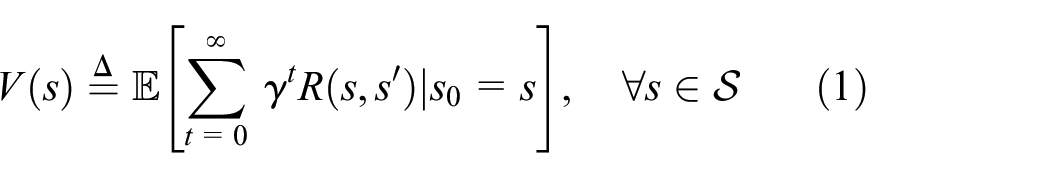
MDP describes the main elements of reinforcement learning in a 5-tuple: $(\mathcal{S},\mathcal{A},P,R,\gamma )$ , where $\mathcal{S}$ means the finite state space of the environment, $\mathcal{A}$ represents the actions set that the agent is likely to take, $P$ is the probability of transition from one state to the next state, $R$ is the reward for moving on to the next state after taking a certain action, and $\gamma$ is a discounting factor, indicating that the further away the moment, the less influence on the present. The goal of reinforcement learning is to maximize the cumulative discount reward, which can be named as value function and expressed by $V(s)$ , and the form is as follows

$$V\left(s\right)\stackrel{\mathrm{\Delta }}{=}\mathbb{E}\left[\sum _{t=0}^{\infty }{\gamma }^{t}R(s,s\prime )|s_0=s\right],\forall s\in \mathcal{S}$$

(1)

where $s\prime$ is the next state of $s$ and $R(s,s\prime )$ is the return from the transition from state $s$ to state $s\prime$ .

The above equation can be written as Bellman equation

$$V\left(s\right)=R(s,s\prime )+\gamma \sum _{s\prime \in \mathcal{S}}{P}_{\mathrm{ss}\prime }V(s\prime ),\forall s\in \mathcal{S}$$

(2)

where $P_{\mathrm{ss}\prime }$ is the probability of transition from state $s$ to $s\prime$ .

In general, we can parameterize the value function $V_{\mu }$ as ${\tilde{V}}_x$ , and the approximation function ${\tilde{V}}_x$ can be used to approximate real value function $V$ . Here we also use linear function approximation, which is more conducive to the subsequent proof. ${\tilde{V}}_x$ takes the form

$$V\left(s\right)\approx {\tilde{V}}_x\left(s\right)=\varphi {\left(s\right)}^{\mathrm{T}}x$$

where $\varphi (s)=({\varphi }_1(s),\dots ,{\varphi }_d(s){)}^{\mathrm{T}}\in {\mathbb{R}}^d$ is basis function of $\tilde{V}(s)$ , and $x\in {\mathbb{R}}^d$ is characteristic parameters. Just to make the notation more concise, let $\mathrm{\Phi }\in {\mathbb{R}}^{|S|\times d}$ as a compact matrix

$$\mathrm{\Phi }=\left[\begin{array}{ccc}|\hfill & \hfill & |\hfill \\ \multicolumn{1}{c}{{\varphi }_1}& \cdots \hfill & {\varphi }_d\hfill \\ \multicolumn{1}{c}{|}& \hfill & |\hfill \end{array}\right]=\left[\begin{array}{ccc}-\hfill & \varphi {\left(1\right)}^{\mathrm{T}}\hfill & -\hfill \\ \multicolumn{1}{c}{⋮}& ⋮\hfill & ⋮\hfill \\ \multicolumn{1}{c}{-}& \varphi {\left(\left|S\right|\right)}^{\mathrm{T}}\hfill & -\hfill \end{array}\right]\in {\mathbb{R}}^{|S|\times d}$$

where $|S|$ is the number of states space, and $d<<|S|$ . Then, we get

$$\tilde{V}\left(x\right)=\mathrm{\Phi }x$$

(3)

Thus, $\nabla {\tilde{V}}_x(s)=\varphi (s)$ and $\nabla \tilde{V}(x)=\mathrm{\Phi }$ . The parameters of TD algorithm update follow the following rules:

$d_t$ is the estimated error at the current time, which is called TD error. It can be written as

$$d_t=r_t+\gamma \tilde{\upsilon }(s_{t+1},x_t)-\tilde{\upsilon }(s_t,x_t)$$

(4)

The parameters are updated as follows

$$x_{t+1}=x_t+\alpha d_t\nabla \tilde{\upsilon }(s_t,x_t)$$

(5)

We can view $d_t\nabla \tilde{\upsilon }(s_t,x_t)$ as the gradient “ $g$ ” in the traditional stochastic gradient descent method, although it’s not a real gradient. Then, we define $g(x_t,{\xi }_t)$ as

$$\begin{array}{c}g(x_t,{\zeta }_t):=d_t\nabla \tilde{\upsilon }(s_t,x_t)\hfill \\ =\varphi \left(s_t\right)[\gamma \varphi {\left(s_{t+1}\right)}^{\mathrm{T}}{x}_t+r_t-\varphi {\left(s_t\right)}^{\mathrm{T}}{x}_t]\hfill \end{array}$$

(6)

where ${\zeta }_t$ is the information observed in environment at the $t$ th state transition, like $(s_t,s_{t+1},r_t)$ .

The parameters update rule can also be written as

$$x_{t+1}=x_t+\alpha g(x_t,{\zeta }_t)$$

(7)

TD(λ) algorithm

The TD( $\lambda$ ) algorithm perfectly explains the relationship between Monte Carlo algorithm and TD algorithm, in which $\lambda \in [0,1]$ . When $\lambda =0$ , it is TD (0) algorithm, and when $\lambda =1$ , it is Monte Carlo algorithm. Generally speaking, when $\lambda$ takes the middle value, it will perform better than the first two extreme algorithms.

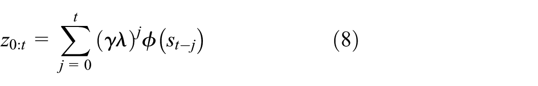
Unlike TD(0), TD( $\lambda$ ) has an extra eligibility traces vector $z\in {\mathbb{R}}^d$ . In TD(0), we used the direction $\varphi (s_t)$ of the eigenvector to updating parameter. In TD( $\lambda$ ), instead of using the direction $\varphi (s_t)$ , the updating parameter uses the direction of the eligibility traces $z_{0:t}$ , and $z_{0:t}$ follows the update function

$$z_{0:t}=\sum _{j=0}^t{\left(\gamma \lambda \right)}^j\varphi \left(s_{t-j}\right)$$

(8)

$z_{0:t}$ is used to capture the influence of each feature on TD error, and by simplifying it, we can write it as

$$z_{0:t}=\gamma \lambda z_{0:t-1}+\varphi \left(s_t\right)$$

(9)

The parameters are updated as follows

$$x_{t+1}=x_t+\alpha d_t{z}_{0:t}$$

(10)

Like TD (0), we can also define $g_t(x_t,z_{0:t})$ , which acts the same as “ $g$ ” in the gradient descent method. The definition of $g_t(x_t,z_{0:t})$ is as follows

$$g_t(x_t,z_{0:t})=d_t{z}_{0:t}$$

(11)

$$\overline{g}(x)=\underset{t\to \infty }{lim}\mathbb{E}\left[d_t{z}_{0:t}\right]$$

(12)

Parameter updates can also be represented by the following equation

$$x_{t+1}=x_t+\alpha g_t(x_t,z_{0:t})$$

(13)

That’s the basics of the original TD( $\lambda$ ) algorithm, but in this article, we consider to add Adam-type algorithm on the original TD( $\lambda$ ). Therefore, in the next section, we will further improve the algorithm.

Algorithm design and assumptions

In this section, we present the main algorithm in detail and propose some basic assumptions for subsequent convergence analysis.

Algorithm design

Our algorithm combines TD( $\lambda$ ) and AMSGrad. ${\beta }_1$ and ${\beta }_2$ are hyper-parameters, and ${\beta }_{1,t}={\beta }_1{\gamma }^t$ . $m_t$ is first-order momentum and ${\upsilon }_t$ is second-order momentum. ${\hat{V}}_t$ is a diagonal matrix composed of ${\hat{\upsilon }}_t$ . Moreover, ${\mathrm{\Pi }}_{D,V_t^{-1/4}}$ is a projection operator onto a norm ball less than $D_{\infty }$ . The details are in Algorithm 1:

Algorithm 1. ADTD( $\lambda$ ): Adaptive TD( $\lambda$ ) under Markov Sampling.

for $t=0,1,2,\dots ,\mathrm{T}$ do   $d_t=(r_t+\gamma \varphi {\left(s_{t+1}\right)}^{\mathrm{T}}{x}_t-\varphi {\left(s_t\right)}^{\mathrm{T}}{x}_t)$   $z_{0:t}=\gamma \lambda z_{0:t-1}+\varphi \left(s_t\right)$   $g_t(x_t,z_{0:t})=d_t{z}_{0:t}$   $m_t={\beta }_{1,t}{m}_{t-1}+(1-{\beta }_{1,t})g_t(x_t,z_{0:t})$   ${\upsilon }_t={\beta }_2{\upsilon }_{t-1}+(1-{\beta }_2)g_t(x_t,z_{0:t})\odot g_t(x_t,z_{0:t})$   ${\hat{\upsilon }}_t=max({\hat{\upsilon }}_{t-1},{\upsilon }_t),{\hat{V}}_t=\mathrm{diag}\left({\hat{\upsilon }}_t\right)$   $x_{t+1}={\mathrm{\Pi }}_{D,V_t^{1/4}}(x_t+{\alpha }_t{\hat{V}}_t^{-1/2}{m}_t)$  where ${\mathrm{\Pi }}_{D,V_t^{1/4}}(x\prime )=\underset{x\in D}{min}\Vert V_t^{1/4}(x\prime -x)\Vert$ end for

Assumptions

We specify some fundamental assumptions, which are also standard assumptions in previous stuides,^24,25,29 and these assumptions always hold throughout the rest of this article.

Assumption 1

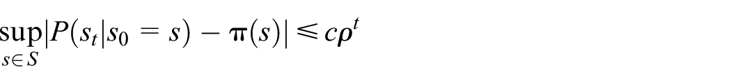
The Markov chain associated is ergodic with $P$ , which also means the Markov chain mixes uniformly, and the following inequality holds

$$\underset{s\in S}{sup}|P(s_t|s_0=s)-\mathrm{\pi }\left(s\right)|\le c{\rho }^t$$

where $\mathrm{\pi }$ is a stationary distribution, and $c\ge 0$ and $0\le \rho \le 1$ are all constant.

Assumption 2

We assume that the matrix $\mathrm{\Phi }$ is linearly independent. Moreover, we assume that $\parallel \varphi (s)\parallel \le 1$ .

Assumption 3

We assume that rewards are uniformly bounded. That is, $|r(s_t,s{\prime }_t)|\le r_{max}$ , where $r_{max}$ is a constant.

Assumption 4

We assume $x_k$ is uniformly bounded. That is, $\parallel x_k\parallel \le D_{\infty }$ , where $D_{\infty }$ is a constant.

Main results

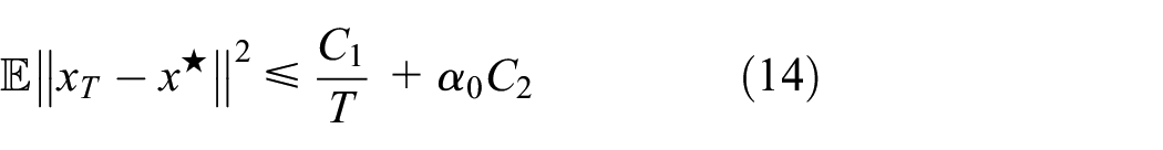
The following content will show the main theoretical results. Specifically, we obtain an upper bound on the error between the estimated parameter and the optimal parameter under the condition of different step-sizes. In the next section, we will prove it in detail.

Theorem 1

Under above Assumptions 1–4, we assume that $\parallel x_i-x_j\parallel \le D_{\infty }$ for any $i,j\in \mathbb{N}$ , and $\parallel \varphi (s)\parallel \le 1$ , $|r(s_t,s{\prime }_t)|\le r_{max}$ , for $\forall s\in \mathcal{S}$ . Moreover, we set $B=(r_{max}+2D_{\infty })/(1-\gamma \lambda )$ , and ${\epsilon }^{*}=max\{min\{\epsilon :(m\rho {)}^{\epsilon }\le {\alpha }_T\},min\{\epsilon :(\gamma \lambda {)}^{\epsilon }\le {\alpha }_T\}\}$ . Let ${\alpha }_t={\alpha }_0$ , where ${\alpha }_0$ is a constant, and $t=1\dots T$ represents the number of iterations. Then, Algorithm 1 satisfies

• (a) when $T\ge 2{\epsilon }^{*}$

$$\mathbb{E}\Vert x_T-x^{★}{\Vert }^2\le \frac{C_1}{T}+{\alpha }_0{C}_2$$

(14)

where

$$\begin{array}{c}{C}_1=\frac{1}{2\omega (1-\kappa )(1-{\beta }_1)}\hfill \\ \{\frac{2{\mathrm{dBD}}_{\infty }^2}{{\alpha }_0}+\frac{{\beta }_1\gamma {\mathrm{dBD}}_{\infty }^2}{(1-\gamma ){\alpha }_0}+\frac{32B^2{\epsilon }^{*2}{\alpha }_0}{B_0}+4{\epsilon }^{*}B{D}_{\infty }-\frac{4{\epsilon }^{*}{B}^2(8{\epsilon }^{*}+3B_0){\alpha }_0}{B_0}\}\hfill \\ C_2=\frac{1}{2\omega (1-\kappa )(1-{\beta }_1)}\left\{\frac{(1+{\beta }_1)B^2+2B^2(8{\epsilon }^{*}+3B_0)}{B_0}\right\}\hfill \end{array}$$

• (b) when $T\le 2{\epsilon }^{*}$

$$\mathbb{E}\Vert x_T-x^{★}{\Vert }^2\le \frac{C_3}{T}+{\alpha }_0{C}_4$$

(15)

where

$$\begin{array}{c}{C}_3=\frac{1}{2\omega (1-\kappa )(1-{\beta }_1)}[\frac{{\beta }_1\gamma {\mathrm{dBD}}_{\infty }^2}{{\alpha }_0(1-\gamma )}+\frac{2{\mathrm{dBD}}_{\infty }^2}{{\alpha }_0}]\hfill \\ C_4=\frac{1}{2\omega (1-\kappa )(1-{\beta }_1)}[\frac{(1+{\beta }_1)B^2+16B^2{\epsilon }^{*}}{B_0}+\frac{B{D}_{\infty }}{{\alpha }_0}]\hfill \end{array}$$

Remark 1

Under the constant step-size and some hyper-parameters, the results of Theorem 1 show that ADTD( $\lambda$ ) can converge to a neighborhood of $x^{*}$ by the rate of $\mathcal{O}(1/T)$ , where $C_1-C_4$ are constants. Moreover, the error upper bounds between the estimated parameter and the optimal parameter are relative to the number of dimensions of ${\hat{V}}_t$ , and the ${\alpha }_0$ is proportional to the size of the neighborhood.

Theorem 2

Under above Assumptions 1–4, we assume that $\parallel x_i-x_j\parallel \le D_{\infty }$ for any $i,j\in \mathbb{N}$ , and $\parallel \varphi (s)\parallel \le 1$ , $|r(s_t,s{\prime }_t)|\le r_{max}$ , for $\forall s\in \mathcal{S}$ . In addition, we initialize ${\hat{\upsilon }}_{0,i}\ge B_0^2$ , ${\beta }_{1,t}={\beta }_1{\gamma }^t$ . We set $B=(r_{max}+2D_{\infty })/(1-\gamma \lambda )$ , and ${\epsilon }^{*}=max\{min\{\epsilon :(m\rho {)}^{\epsilon }\le {\alpha }_T\},min\{\epsilon :(\gamma \lambda {)}^{\epsilon }\le {\alpha }_T\}\}$ , let ${\alpha }_t={\alpha }_0/(\sqrt{t}+1)$ , where $\alpha$ is a constant, and $t=1\dots T$ is the number of iterations. Then, we have

• (a) when $T\ge 2{\epsilon }^{*}$

$$\mathbb{E}\Vert x_T-x^{★}{\Vert }^2\le \frac{C_5}{\sqrt{T}}+\frac{C_6}{T}+{\alpha }_0{C}_7$$

(16)

where

$$\begin{array}{l}{C}_5:\frac{dB{D}_{\infty }^2}{2{\alpha }_0\omega \left(1-\kappa \right)\left(1-{\beta }_1\right)}\\ C_6:\frac{1}{2\omega \left(1-\kappa \right)\left(1-{\beta }_1\right)}\\ \{\frac{dB{D}_{\infty }^2}{{\alpha }_0}+\frac{{\beta }_{1}dB{D}_{\infty }^2}{{\alpha }_0{(1-\gamma )}^2}+\frac{32B^2{\alpha }_0{\epsilon }^{\ast 2}}{B_0}+4{\epsilon }^{\ast }B{D}_{\infty }-\frac{4{\epsilon }^{\ast }{B}^2(8{\epsilon }^{\ast }+3B_0){\alpha }_0}{B_0}\}\\ C_7:\frac{1}{2\omega \left(1-\kappa \right)\left(1-{\beta }_1\right)}\left\{\frac{\left(1+{\beta }_1\right)B^2}{B_0}+\frac{2B^2\left(8{\epsilon }^{\ast }+3B_0\right)}{B_0}\right\}\end{array}$$

• (b) when $T\le 2{\epsilon }^{*}$

$$\mathbb{E}\Vert x_T-x^{★}{\Vert }^2\le \frac{C_5}{\sqrt{T}}+\frac{C_8}{T}+{\alpha }_0{C}_4$$

where

$$C_8:=\frac{1}{2\omega T(1-\kappa )(1-{\beta }_1)}[\frac{{\mathrm{dBD}}_{\infty }^2}{{\alpha }_0}+\frac{{\beta }_1\mathrm{dB}{D}_{\infty }}{{\alpha }_0{(1-\gamma )}^2}]$$

Remark 2

Similar to Theorem 1, $C_5-C_{10}$ are also constants and time-independent; we can adjust ${\alpha }_t$ to make a trade-off between convergence speed and convergence accuracy. Let ${\alpha }_t={\alpha }_0/(\sqrt{t}+1)$ ; ADTD( $\lambda$ ) converges to a neighborhood of $x^{*}$ by the rate of $\tilde{\mathcal{O}}(1/\sqrt{T})$ . Moreover, $\mathbb{E}\parallel x_T-x^{★}{\parallel }^2$ is relative to the number of dimensions of ${\hat{V}}_t$ .

Convergence analysis

In this section, we will analyze the convergence performance of ADTD( $\lambda$ ). In order to get Theorem 1 and Theorem 2, we need some Lemmas to set the stage first.

Lemma 1

To limit the update direction of $\mathrm{TD}(\lambda )$ , for $\forall x\in {\mathbb{R}}^d$ , we have (Lemma 3) ²⁵

$$(x^{*}-x)\overline{g}\left(x\right)\ge (1-\kappa )\Vert V_{x^{*}}-V_x{\Vert }^2\ge (1-\kappa )\omega \Vert x^{*}-x{\Vert }^2$$

(17)

where $\kappa :=(\gamma (1-\lambda ))/(1-\gamma \lambda )$ and $\omega \ge 0$ .

Since the gradient estimation is biased under Markov sampling, we also use information theory techniques to control this bias in this article.

Lemma 2

Under Assumption 1, we assume that A and B are two random variables, $t\in \mathbb{N}$ , and $\epsilon \ge 0$ ; A to B can be described as a Markov process, such that $A\to s_t\to s_{t+\epsilon }\to B$ . Let $A\prime$ and $B\prime$ are independent, drawn from the marginal distributions of $A$ and $B$ , so $\mathbb{P}(A\prime =·,B\prime =·)=\mathbb{P}(A=·)\times \mathbb{P}(B=·).$ For any bounded function $f$ , we have (information theory technology, Lemma 3) ²⁵

$$\left[f(A,B)\right]-\mathbb{E}\left[f(A\prime ,B\prime )\right]|\le 2\Vert f{\Vert }_{\infty }c{\rho }^{\epsilon }$$

(18)

where $c>0$ and $\rho \in (0,1)$ .

Furthermore, in order to obtain the final conclusion, we need to get the following results. To ensure the integrity of the article, we repeat the proof of Lemma 3.

Lemma 3

Under Assumptions 2–4, for $\forall s\in \mathcal{S}$ , we assume that $\parallel \varphi (s)\parallel \le 1$ , $|r(s_t,s{\prime }_t)|\le r_{max}$ . Then, for $\forall x\in {\mathbb{R}}^d$ , we have (Lemma 17) ²⁵

$$\Vert g_t(x_t,z_{0:t})\Vert \le B,\Vert \overline{g}(x)\Vert \le B$$

(19)

Proof

According to the definition of $g_t(x_t,z_{0:t})$ , we have

$$\Vert g_t(x,z_{0:t})\Vert =\Vert d_t\left(x\right)z_{0:t}\Vert =\left|d_t\left(x\right)\right|\Vert z_{0:t}\Vert$$

(20)

and then take the bounds of $|d_t(x)|$ and $\parallel z_{0:t}\parallel$ , respectively

$$\begin{array}{c}\multicolumn{1}{c}{\left|d_t\left(x\right)\right|=|\gamma \varphi {\left(s_{t+1}\right)}^{\mathrm{T}}x+r_t-\varphi {\left(s_t\right)}^{\mathrm{T}}x|}\\ \le \Vert \varphi \left(s_{t+1}\right)\Vert \Vert x\Vert +r_{max}+\Vert \varphi \left(s_t\right)\Vert \Vert x\Vert \hfill \\ \le (r_{max}+2D_{\infty })\hfill \end{array}$$

(21)

where the first equation holds because of the definition of $d_t(x)$ , the first inequality is based on the norm inequality, and the last inequality uses Assumption 1 that $\parallel \varphi (s_t)\parallel \le 1$ , $\parallel x\parallel \le D_{\infty }$ , and $|r_t|\le r_{max}$ .

Next bound $\parallel z_{0:t}\parallel$

$$\begin{array}{c}\Vert z_{0:t}{\Vert }^2=\Vert \sum _{j=0}^t{\left(\gamma \lambda \right)}^j\varphi \left(s_{t-j}\right){\Vert }^2\hfill \\ \le {\left(\sum _{j=0}^t{\left(\gamma \lambda \right)}^j\right)}^2\le {\left(\sum _{j=0}^{\infty }{\left(\gamma \lambda \right)}^j\right)}^2=\frac{1}{{(1-\gamma \lambda )}^2}\hfill \end{array}$$

(22)

where the first inequality holds since $\parallel \varphi (s_{t-j})\parallel \le 1$ . Plugging (21) and (22) into (20), we can obtain

$$\Vert g_t(x,z_{0:t})\Vert =\left|d_t\left(x\right)\right|\Vert z_{0:t}\Vert \le \frac{(r_{max}+2D_{\infty })}{(1-\gamma \lambda )}$$

(23)

We note that $B=(r_{max}+2D_{\infty })/(1-\gamma \lambda )$ . Similarly, we can get $\parallel d_t(x)z_{l:t}\parallel \le B$ for $l\le t$ . Let $l\to -\infty$ ; we can get $\parallel d_t(x)z_{-\infty :t}\parallel \le B$ . As $\overline{g}(x)=\mathbb{E}[d_t(x)z_{-\infty :t}]$ , so $\parallel \overline{g}(x)\parallel \le B$ , we omit this proof here.

Next, we need to get some useful bounds that will prepare for the final theorem proof.

Lemma 4

Under Assumptions 2–4, for $\forall s\in \mathcal{S}$ , we assume that $\parallel \varphi (s)\parallel \le 1$ , $|r(s_t,s{\prime }_t)|\le r_{max}$ . By Lemma 3, we have $B=(r_{max}+2D_{\infty })/(1-\gamma \lambda )$ . For any $x\in {\mathbb{R}}^d$ , we can obtain the bound as follows

$$\Vert m_t\Vert \le B,\Vert {\hat{\upsilon }}_t{\Vert }_{\infty }\le B^2$$

(24)

Proof

We use the inductive hypothesis to bound $\parallel m_t\parallel$ and $\parallel {\hat{\upsilon }}_t{\parallel }_{\infty }$ . We first assume that $\parallel m_0\parallel =0\le B$ and $\parallel m_t\parallel \le B$ ; by the definition of $m_{t+1}$ , we obtain

$$\begin{array}{c}\Vert m_{t+1}\Vert \Vert {\beta }_{1,t+1}{m}_t+(1-{\beta }_{1,t+1})g_{t+1}(x_{t+1},z_{0:t+1}))\Vert \hfill \\ \le {\beta }_{1,t+1}\Vert m_t\Vert +(1-{\beta }_{1,t+1})\Vert g_{t+1}(x_{t+1},z_{0:t+1}))\Vert \hfill \\ \le {\beta }_{1,t+1}B+(1-{\beta }_{1,t+1})B=B\hfill \end{array}$$

(25)

Therefore, we obtain $\parallel m_t\parallel \le B$ , for $t\ge 0$ .

Next, we bound $\parallel {\hat{\upsilon }}_t{\parallel }_{\infty }\le B^2$ . We also first assume that $\parallel {\upsilon }_0{\parallel }_{\infty }=\parallel {\hat{\upsilon }}_0{\parallel }_{\infty }=0\le B^2$ , and $\parallel {\upsilon }_t{\parallel }_{\infty }\le B^2$ . By the definition of ${\upsilon }_{t+1}$ , we obtain

$$\begin{array}{c}\multicolumn{1}{c}{\Vert {\upsilon }_{t+1}{\Vert }_{\infty }=\Vert {\beta }_2{\upsilon }_t+(1-{\beta }_2)g_{t+1}(x_{t+1},z_{0:t+1})){\Vert }_{\infty }}\\ \le {\beta }_2\Vert {\upsilon }_t{\Vert }_{\infty }+(1-{\beta }_2)\Vert g_{t+1}(x_{t+1},z_{0:t+1})){\Vert }_{\infty }\hfill \\ \le {\beta }_2{B}^2+(1-{\beta }_2)B^2=B^2\hfill \end{array}$$

(26)

where the second inequality holds due to Lemma 3

$$\Vert g_{t+1}(x_{t+1},z_{0:t+1})){\Vert }_{\infty }\le \Vert g_{t+1}(x_{t+1},z_{0:t+1}))\Vert \le B$$

(27)

We have $\parallel {\hat{\upsilon }}_{t+1}{\parallel }_{\infty }=max\{\parallel {\hat{\upsilon }}_t{\parallel }_{\infty },\parallel {\upsilon }_{t+1}{\parallel }_{\infty }\}\le B^2$ . Therefore, we obtain that $\parallel {\hat{\upsilon }}_t{\parallel }_{\infty }\le B^2$ , for all $t\ge 0$ .

Next, we will discuss the function ${\xi }_t$ , which represents the error in the updating direction at instant $t$ . We define it as follows

$${\xi }_t(x,z_{l:t})={(d_t\left(x\right)z_{l:t}-\overline{g}\left(x\right))}^{\mathrm{T}}(x-x^{*})$$

(28)

where $x\in {\mathbb{R}}^d$ , and $l\le t$ .

To obtain $E[{\xi }_t(x,z_{l:t})]$ , we first need to obtain some properties of $|{\xi }_t(x,z_{l:t})|$ .

Lemma 5

Under Assumptions 2–4, for $\forall s\in \mathcal{S}$ , we assume that $\parallel \varphi (s)\parallel \le 1$ , $|r(s_t,s{\prime }_t)|\le r_{max}$ . Besides, $\parallel x_i-x_j\parallel \le D_{\infty }$ for any $i,j\in \mathbb{N}$ . Combining the results of Lemma 3 and Lemma 4, for any $x\in {\mathbb{R}}^d$ , we can obtain the properties as follows (Lemma 19) ²⁵

$$\begin{array}{c}(a)|{\xi }_t(x,z_{l:t})|\le 2B{D}_{\infty }.\hfill \\ (b)|{\xi }_t(x,z_{0:t})-{\xi }_t(x,z_{t-\epsilon :t})|\le B{D}_{\infty }(\gamma \lambda {)}^{\epsilon },\mathrm{for}\forall \epsilon \le t.\hfill \\ (c)|{\xi }_t(x,z_{0:t})-{\xi }_t(x,z_{-\infty :t})|\le B{D}_{\infty }(\gamma \lambda {)}^t.\hfill \\ (d)|{\xi }_t(x,z_{l:t})-{\xi }_t(x\prime ,z_{l:t})|\le 4B\parallel (x-x\prime )\parallel .\hfill \end{array}$$

Proof

We just prove the part ( $d$ ) of Lemma 5 here. That is to say, ${\xi }_t(x,z_{l:t})$ satisfies $L$ -Lipschitz property. The other parts of Lemma 5 are similar to Bhandari et al. ²⁵ and we omit them here

$$\begin{array}{c}|{\xi }_t(x,z_{l:t})-{\xi }_t(x\prime ,z_{l:t})|\hfill \\ =|{(d_t\left(x\right)z_{l:t}-\overline{g}\left(x\right))}^{\mathrm{T}}(x-x^{*})-{(d_t(x\prime )z_{l:t}-\overline{g}(x\prime ))}^{\mathrm{T}}(x\prime -x^{*})|\hfill \\ \le \Vert d_t\left(x\right)z_{l:t}-\overline{g}\left(x\right)\Vert \Vert x-x\prime \Vert \hfill \\ +\Vert x\prime -x^{*}\Vert \Vert (d_t\left(x\right)z_{l:t}-\overline{g}\left(x\right))-(d_t(x\prime )z_{l:t}-\overline{g}(x\prime ))\Vert \hfill \\ \le [\Vert d_t\left(x\right)z_{l:t}\Vert +\Vert \overline{g}\left(x\right)\Vert ]\Vert x-x\prime \Vert \hfill \\ +\Vert x\prime -x^{*}\Vert \Vert (d_t\left(x\right)z_{l:t}-\overline{g}\left(x\right))-(d_t(x\prime )z_{l:t}-\overline{g}(x\prime ))\Vert \hfill \\ \le 2B\Vert x-x\prime \Vert +D_{\infty }[\Vert z_{l:t}(d_t\left(x\right)-d_t(x\prime ))\Vert +\Vert \overline{g}\left(x\right)-\overline{g}(x\prime )\Vert ]\hfill \\ \le 2B\Vert x-x\prime \Vert +\frac{4D_{\infty }}{(1-\gamma \lambda )}\Vert x-x\prime \Vert \le 4B\Vert x-x\prime \Vert \hfill \end{array}$$

(29)

the first inequality holds since $|a^{\mathrm{T}}b-c^{\mathrm{T}}d|=|a^{\mathrm{T}}(b-d)+d^{\mathrm{T}}(a-c)|\le \parallel a\parallel \parallel b-d\parallel +\parallel d\parallel \parallel a-c\parallel$ , where $a,b,c,\mathrm{and}d$ are four vectors. The last inequality establishes because $2D_{\infty }/(1-\gamma \lambda )\le B$ . In the penultimate inequality, we can easily prove $\parallel z_{l:t}(d_t(x)-d_t(x\prime ))\parallel$ and $\parallel \overline{g}(x)-\overline{g}(x\prime )\parallel$ as follows

$$\begin{array}{c}\Vert z_{l:t}(d_t\left(x\right)-d_t(x\prime ))\Vert \le \Vert z_{l:t}\Vert \left|(d_t\left(x\right)-d_t(x\prime ))\right|\hfill \\ \le \Vert \sum _{j=0}^{\infty }{\left(\gamma \lambda \right)}^j\varphi \left(s_{t-j}\right)\Vert \left|(d_t\left(x\right)-d_t(x\prime ))\right|\hfill \\ \le \frac{1}{(1-\gamma \lambda )}\left|{(\gamma \varphi \left(s{\prime }_t\right)-\varphi \left(s_t\right))}^{\mathrm{T}}(x-x\prime )\right|\hfill \\ \le \frac{(\Vert \varphi \left({s\prime }_t\right)\Vert +\Vert \varphi \left(s_t\right)\Vert )}{(1-\gamma \lambda )}\Vert x-x\prime \Vert \le \frac{2}{(1-\gamma \lambda )}\Vert x-x\prime \Vert \hfill \end{array}$$

(30)

Similarly, we can obtain $\parallel \overline{g}(x)-\overline{g}(x\prime )\parallel \le 2/(1-\gamma \lambda )\parallel x-x\prime \parallel$ .

Using Lemma 5, we obtain some properties of $|{\xi }_t(x_t,z_{0:t})|$ , and then we can solve for $\mathbb{E}[{\xi }_t(x_t,z_{0:t})]$ .

Lemma 6

Under Assumptions 1–4 and Lemma 5, considering the step-size sequence is non-increasing, ${\epsilon }^{*}=max\{min\{\epsilon :(m\rho {)}^{\epsilon }\le {\alpha }_T\},min\{\epsilon :(\gamma \lambda {)}^{\epsilon }\le {\alpha }_T\}\}$ , we can obtain

• (1) For $2{\epsilon }^{*}<t\le T$

$$\mathbb{E}\left[{\xi }_t(x_t,z_{0:t})\right]\le \frac{B^2(8{\epsilon }^{*}+3B_0){\alpha }_{t-2{\epsilon }^{*}}}{B_0}$$

(31)

• (2) For all $t\in \mathbb{N}$

$$\mathbb{E}\left[{\xi }_t(x_t,z_{0:t})\right]\le \frac{4B^2}{B_0}\sum _{j=0}^{t-1}{\alpha }_j+B{D}_{\infty }{\left(\gamma \lambda \right)}^t$$

(32)

• (3) For $0\le t\le 2{\epsilon }^{*}$

$$\mathbb{E}\left[{\xi }_t(x_t,z_{0:t})\right]\le \frac{8B^2{\alpha }_0{\epsilon }^{*}}{B_0}+B{D}_{\infty }{\left(\gamma \lambda \right)}^t$$

(33)

Proof

• Case (1): When $t>2{\epsilon }^{*}$ , we obtain

$$\begin{array}{c}\multicolumn{1}{c}{\mathbb{E}\left[{\xi }_t(x_t,z_{0:t})\right]\le \underset{I}{\underbrace{|\mathbb{E}\left[{\xi }_t(x_t,z_{0:t})\right]-\mathbb{E}\left[{\xi }_t(x_{t-2\epsilon },z_{0:t})\right]|}}}\\ +\underset{\mathrm{II}}{\underbrace{|\mathbb{E}\left[{\xi }_t(x_{t-2\epsilon },z_{0:t})\right]-\mathbb{E}\left[{\xi }_t(x_{t-2\epsilon },z_{t-\epsilon :t})\right]|}}\hfill \\ +\underset{\mathrm{III}}{\underbrace{\left|\mathbb{E}\left[{\xi }_t(x_{t-2\epsilon },z_{t-\epsilon :t})\right]\right|}}\hfill \end{array}$$

(34)

To get the bound on $\mathbb{E}[{\xi }_t(x_t,z_{0:t})]$ , we have to figure out the three terms, respectively.

• Item I: According to the Lipschitz property of ${\xi }_t(x_t,z_{0:t})$ in Lemma 5, we can obtain

$$\begin{array}{c}\multicolumn{1}{c}{|{\xi }_t(x_t,z_{0:t})-{\xi }_t(x_{t-2\epsilon },z_{0:t})|\le 4B\Vert x_t-x_{t-2\epsilon }\Vert }\\ \le \frac{4B^2}{B_0}\sum _{j=t-2\epsilon }^{t-1}{\alpha }_j\hfill \end{array}$$

(35)

In equation (35), the term $\parallel x_t-x_{t-2\epsilon }\parallel$ is proved as follows

$$\begin{array}{c}\multicolumn{1}{c}{\Vert x_t-x_{t-2\epsilon }\Vert \le \sum _{j=t-2\epsilon }^{t-1}\Vert {\mathrm{\Pi }}_{D,V_j^{1/4}}(x_{j+1}+{\alpha }_j{\hat{V}}_j^{-1/2}{m}_j)-x_j\Vert }\\ \le \sum _{j=t-2\epsilon }^{t-1}{\alpha }_j\Vert V_j^{-1/2}{m}_j\Vert \le \frac{B}{B_0}\sum _{j=t-2\epsilon }^{t-1}{\alpha }_j\hfill \end{array}$$

(36)

where the last inequality holds since

$$\Vert {\hat{V}}_t^{-1/2}{m}_t{\Vert }^2=\sum _{i=1}^d\frac{m_{t,i}^2}{{\hat{\upsilon }}_{t,i}}\le \frac{1}{B_0^2}\sum _{i=1}^d{m}_{t,i}^2\le \frac{B^2}{B_0^2}$$

(37)

we assume that ${\hat{\upsilon }}_{t,i}\ge {\hat{\upsilon }}_{1,i}\ge B_0^2,\forall t,\forall i.$

• Item II: By Lemma 5, we can directly obtain

$$|\mathbb{E}\left[{\xi }_t(x_{t-2\epsilon },z_{0:t})\right]-\mathbb{E}\left[{\xi }_t(x_{t-2\epsilon },z_{t-\epsilon :t})\right]|\le B{D}_{\infty }{\left(\gamma \lambda \right)}^{\epsilon }$$

(38)

• Item III: Using the information theory technology to bound $\mathbb{E}[{\xi }_t(x_{t-2\epsilon },z_{t-\epsilon :t})]$ , we define that ${\vartheta }_{t-\epsilon :t}$ is a state sequence from $s_{t-\epsilon }$ to $s_t$ ; it is also a Markov chain

$$x_{t-2\epsilon }\to s_{t-2\epsilon }\to s_{t-\epsilon }\to s_t\to O_t$$

(39)

We define a function $h(x_{t-2\epsilon },{\vartheta }_{t-\epsilon :t})$

$$h(x_{t-2\epsilon },{\vartheta }_{t-\epsilon :t}):={\xi }_t(x_{t-2\epsilon },z_{t-\epsilon :t})$$

(40)

where random variables $x{\prime }_{t-2\epsilon }$ and $\vartheta {\prime }_{t-\epsilon :t}$ were drawn independently from the marginal distributions of $x_{t-2\epsilon }$ and ${\vartheta }_{t-\epsilon :t}$ , respectively. So $\mathbb{P}(x{\prime }_{t-2\epsilon }=·,\vartheta {\prime }_{t-\epsilon :t}=·)=\mathbb{P}(x_{t-\epsilon }=·)\times \mathbb{P}({\vartheta }_{t-\epsilon :t}=·)$

$$\begin{array}{c}\left|\mathbb{E}\left[{\xi }_t(x_{t-2\epsilon },z_{t-\epsilon :t})\right]\right|=\left|\mathbb{E}\left[h(x_{t-2\epsilon },{\vartheta }_{t-\epsilon :t})\right]\right|\hfill \\ \le |\mathbb{E}\left[h(x_{t-2\epsilon },{\vartheta }_{t-\epsilon :t})\right]-\mathbb{E}\left[h({x\prime }_{t-2\epsilon },{\vartheta \prime }_{t-\epsilon :t})\right]|\hfill \\ +\left|\mathbb{E}\left[h({x\prime }_{t-2\epsilon },{\vartheta \prime }_{t-\epsilon :t})\right]\right|\hfill \end{array}$$

(41)

According to Lemma 2, we get

$$|\mathbb{E}\left[h(x_{t-2\epsilon },{\vartheta }_{t-\epsilon :t})\right]-\left[h({x\prime }_{t-2\epsilon },{\vartheta \prime }_{t-\epsilon :t})\right]\mathbb{E}|\le 4B{D}_{\infty }c{\rho }^{\epsilon }$$

(42)

Using Lemma 5, we obtain

$$\begin{array}{c}\mathbb{E}[h(x,{\vartheta }_{t-\epsilon :t})]={(\mathbb{E}\left[d_t\left(x\right)z_{t-\epsilon :t}\right]-\overline{g}\left(x\right))}^{\mathrm{T}}(x-x^{*})\hfill \\ \le \left|{(d_t(x)z_{-\infty :t-\epsilon })}^{\mathrm{T}}(x-x^{*})\right|\le B{D}_{\infty }{\left(\gamma \lambda \right)}^{\epsilon }\hfill \end{array}$$

(43)

Plugging (42) and (43) into (41), we can obtain

$$\left|\mathbb{E}\left[{\xi }_t(x_{t-2\epsilon },z_{t-\epsilon :t})\right]\right|\le 4B{D}_{\infty }c{\rho }^{\epsilon }+B{D}_{\infty }{\left(\gamma \lambda \right)}^{\epsilon }$$

(44)

Now, let $\epsilon ={\epsilon }^{*}$ , merging (35), (38), and (44), we can obtain

$$\begin{array}{c}\mathbb{E}\left[{\xi }_t(x_t,z_{0:t})\right]\le \frac{4B^2}{B_0}\sum _{j=t-2\epsilon }^{t-1}{\alpha }_j+4B{D}_{\infty }c{\rho }^{\epsilon }+2B{D}_{\infty }{\left(\gamma \lambda \right)}^{\epsilon }\hfill \\ \le \frac{8B^2{\epsilon }^{*}{\alpha }_{t-2{\epsilon }^{*}}}{B_0}+3B^2{\alpha }_T\le \frac{B^2(8{\epsilon }^{*}+3B_0){\alpha }_{t-2{\epsilon }^{*}}}{B_0}\hfill \end{array}$$

(45)

where the second inequality holds because step-size sequence is non-increasing, $2D_{\infty }\le B$ , and $(\gamma \lambda {)}^{\epsilon }\le {\alpha }_T$ , $c{\rho }^{\epsilon }\le {\alpha }_T$ . The last inequality follows from ${\alpha }_T\le {\alpha }_{t-2{\epsilon }^{*}}$ .

• Case (2): For all $t\in \mathbb{N}$ , we obtain

$$\begin{array}{c}\mathbb{E}\left[{\xi }_t(x_t,z_{0:t})\right]\le |\mathbb{E}\left[{\xi }_t(x_t,z_{0:t})\right]-\mathbb{E}\left[{\xi }_t(x_0,z_{0:t})\right]|\hfill \\ +|\mathbb{E}\left[{\xi }_t(x_0,z_{0:t})\right]-\mathbb{E}\left[{\xi }_t(x_0,z_{-\infty :t})\right]|+\left|\mathbb{E}\left[{\xi }_t(x_0,z_{-\infty :t})\right]\right|\hfill \end{array}$$

(46)

Combining (35) and (38), we can obtain

$$\begin{array}{c}|\mathbb{E}\left[{\xi }_t(x_t,z_{0:t})\right]-\mathbb{E}\left[{\xi }_t(x_0,z_{0:t})\right]|\hfill \\ +|\mathbb{E}\left[{\xi }_t(x_0,z_{0:t})\right]-\mathbb{E}\left[{\xi }_t(x_0,z_{-\infty :t})\right]|\hfill \\ \le \frac{4B^2}{B_0}\sum _{j=0}^{t-1}{\alpha }_j+B{D}_{\infty }{\left(\gamma \lambda \right)}^t\hfill \end{array}$$

(47)

For the last term of (46)

$$\begin{array}{c}\multicolumn{1}{c}{\mathbb{E}\left[{\xi }_t(x_0,z_{-\infty :t})\right]={(\mathbb{E}\left[d_t\left(x_0\right)z_{-\infty :t}\right]-\overline{g}\left(x_0\right))}^{\mathrm{T}}(x_0-x^{*})=0}\end{array}$$

(48)

This last equation follows from $\overline{g}(x)=\mathbb{E}[d_t(x)z_{-\infty :t}]$ .

Therefore, combining (47) with (48), we can obtain

$$\mathbb{E}\left[{\xi }_t(x_t,z_{0:t})\right]\le \frac{4B^2}{B_0}\sum _{j=0}^{t-1}{\alpha }_j+B{D}_{\infty }{\left(\gamma \lambda \right)}^t,\forall t\in \mathbb{N}$$

(49)

• Case (3): For $t\le 2{\epsilon }^{*}$ , similar to case (2), we can easily obtain

$$\begin{array}{c}\mathbb{E}\left[{\xi }_t(x_t,z_{0:t})\right]\le \frac{4B^2}{B_0}\sum _{j=0}^{t-1}{\alpha }_j+B{D}_{\infty }{\left(\gamma \lambda \right)}^t\hfill \\ \le \frac{4B^{2}t{\alpha }_0}{B_0}+B{D}_{\infty }{\left(\gamma \lambda \right)}^t\hfill \\ \le \frac{8B^2{\epsilon }^{*}{\alpha }_0}{B_0}+B{D}_{\infty }{\left(\gamma \lambda \right)}^t\hfill \end{array}$$

(50)

where the second and the last inequality holds since $\sum _{j=0}^{t-1}{\alpha }_j\le t{\alpha }_0$ and $t\le 2{\epsilon }^{*}.$

With the assumptions and lemmas in mind, we start to prove Theorem 1; detailed proofs are shown below.

Proof

First, according to the definition of $x_{t+1}$ , we have

$$\begin{array}{c}\Vert {\hat{V}}_t^{1/4}(x_{t+1}-x^{★}){\Vert }^2=\Vert {\mathrm{\Pi }}_{\mathcal{D},{\hat{V}}_t^{1/4}}{\hat{V}}_t^{1/4}(x_t-{\alpha }_t{\hat{V}}_t^{-1/2}{m}_t-x^{★}){\Vert }^2\hfill \\ \le \Vert {\hat{V}}_t^{1/4}(x_t-{\alpha }_t{\hat{V}}_t^{-1/2}{m}_t-x^{★}){\Vert }^2=\Vert {\hat{V}}_t^{1/4}(x_t-x^{★}){\Vert }^2\hfill \\ +\Vert {\alpha }_t{\hat{V}}_t^{-1/4}{m}_t{\Vert }^2-2{\alpha }_t{(x_t-x^{★})}^{\mathrm{T}}{m}_t=\Vert {\hat{V}}_t^{1/4}(x_t-x^{★}){\Vert }^2\hfill \\ +\Vert {\alpha }_t{\hat{V}}_t^{-1/4}{m}_t{\Vert }^2-2{\alpha }_t{(x_t-x^{★})}^{\mathrm{T}}[{\beta }_{1t}{m}_{t-1}+(1-{\beta }_{1t})g_t(x_t,z_{0:t})]\hfill \\ \le \Vert {\hat{V}}_t^{1/4}(x_t-x^{★}){\Vert }^2+\Vert {\alpha }_t{\hat{V}}_t^{-1/4}{m}_t{\Vert }^2-2{\alpha }_t(1-{\beta }_{1t}){(x_t-x^{★})}^{\mathrm{T}}\hfill \\ g_t(x_t,z_{0:t})+{\alpha }_t{\beta }_{1t}(\frac{1}{{\alpha }_t}{\Vert {\hat{V}}_t^{1/4}(x_t-x^{★})\Vert }^2+{\alpha }_t{\Vert {\hat{V}}_t^{-1/4}{m}_{t-1}\Vert }^2)\hfill \\ =\Vert {\hat{V}}_t^{1/4}(x_t-x^{★}){\Vert }^2+\Vert {\alpha }_t{\hat{V}}_t^{-1/4}{m}_t{\Vert }^2-2{\alpha }_t(1-{\beta }_{1t}){(x_t-x^{★})}^{\mathrm{T}}\hfill \\ g_t(x_t,z_{0:t})+{\beta }_{1t}\Vert {\hat{V}}_t^{1/4}(x_t-x^{★}){\Vert }^2+{\alpha }_t^2{\beta }_{1t}\Vert {\hat{V}}_t^{-1/4}{m}_{t-1}{\Vert }^2\hfill \\ \le \Vert {\hat{V}}_t^{1/4}(x_t-x^{★}){\Vert }^2+{\alpha }_t^2(1+{\beta }_{1t})\Vert {\hat{V}}_t^{-1/4}{m}_t{\Vert }^2+{\beta }_{1t}\Vert {\hat{V}}_t^{1/4}(x_t-x^{★}){\Vert }^2\hfill \\ -2{\alpha }_t(1-{\beta }_{1t}){(x_t-x^{★})}^{\mathrm{T}}{g}_t(x_t,z_{0:t})\hfill \end{array}$$

(51)

where the second inequality is established due to Young’s inequality and the last inequality holds because $m_{t-1}\le m_t$ .

Next, we take the expectation of (51)

$$\begin{array}{c}\mathbb{E}\Vert {\hat{V}}_t^{1/4}(x_{t+1}-x^{★}){\Vert }^2\le \mathbb{E}\Vert {\hat{V}}_t^{1/4}(x_t-x^{★}){\Vert }^2\hfill \\ +{\alpha }_t^2(1+{\beta }_{1t})\mathbb{E}\Vert {\hat{V}}_t^{-1/4}{m}_t{\Vert }^2+{\beta }_{1t}\mathbb{E}\Vert {\hat{V}}_t^{1/4}(x_t-x^{★}){\Vert }^2\hfill \\ -2{\alpha }_t(1-{\beta }_{1t})\mathbb{E}\left[{(x_t-x^{★})}^{\mathrm{T}}{g}_t(x_t,z_{0:t})\right]\hfill \\ =\mathbb{E}\Vert {\hat{V}}_t^{1/4}(x_t-x^{★}){\Vert }^2+{\alpha }_t^2(1+{\beta }_{1t})\Vert {\hat{V}}_t^{-1/4}{m}_t{\Vert }^2\hfill \\ +{\beta }_{1t}\mathbb{E}\Vert {\hat{V}}_t^{1/4}(x_t-x^{★}){\Vert }^2-2{\alpha }_t(1-{\beta }_{1t})\mathbb{E}\left[{(x_t-x^{★})}^{\mathrm{T}}{\overline{g}}_t(x_t,z_{0:t})\right]\hfill \\ +2{\alpha }_t(1-{\beta }_{1t})\mathbb{E}[{(x_t-x^{★})}^{\mathrm{T}}\left({\overline{g}}_t(x_t,z_{0:t})\right)-g_t(x_t,z_{0:t})]\hfill \\ \le \mathbb{E}\Vert {\hat{V}}_t^{1/4}(x_t-x^{★}){\Vert }^2+{\alpha }_t^2(1+{\beta }_{1t})\Vert {\hat{V}}_t^{-1/4}{m}_t{\Vert }^2\hfill \\ +{\beta }_{1t}\mathbb{E}\Vert {\hat{V}}_t^{1/4}(x_t-x^{★}){\Vert }^2+2{\alpha }_t(1-{\beta }_{1t})\mathbb{E}\left[{\xi }_t(x_t,z_{0:t})\right]\hfill \\ -2{\alpha }_t\omega (1-{\beta }_{1t})(1-\kappa )\mathbb{E}\Vert x_t-x^{★}{\Vert }^2\hfill \\ \le \mathbb{E}\Vert {\hat{V}}_t^{1/4}(x_t-x^{★}){\Vert }^2+{\alpha }_t^2(1+{\beta }_{1t})\Vert {\hat{V}}_t^{-1/4}{m}_t{\Vert }^2\hfill \\ +{\beta }_{1t}\mathbb{E}\Vert {\hat{V}}_t^{1/4}(x_t-x^{★}){\Vert }^2+2{\alpha }_t(1-{\beta }_{1t})\mathbb{E}\left[{\xi }_t(x_t,z_{0:t})\right]\hfill \\ -2{\alpha }_t\omega (1-{\beta }_1)(1-\kappa )\mathbb{E}\Vert x_t-x^{★}{\Vert }^2\hfill \\ \le \mathbb{E}\Vert {\hat{V}}_t^{1/4}(x_t-x^{★}){\Vert }^2+{\alpha }_t^2(1+{\beta }_1)\Vert {\hat{V}}_t^{-1/4}{m}_t{\Vert }^2+{\beta }_{1t}{\mathrm{dBD}}_{\infty }^2\hfill \\ +2{\alpha }_t(1-{\beta }_{1t})\mathbb{E}\left[{\xi }_t(x_t,z_{0:t})\right]-2{\alpha }_t\omega (1-{\beta }_1)(1-\kappa )\mathbb{E}\Vert x_t-x^{★}{\Vert }^2\hfill \end{array}$$

(52)

where the second inequality holds because of Lemma 1 and the third inequality holds since ${\beta }_{1,t}\le {\beta }_1\le 1$ . The last inequality is obtained by Lemma 5 and $\parallel {\hat{V}}_t\parallel \le \sqrt{d}\parallel {\hat{V}}_t{\parallel }_{\infty }\le \sqrt{d}{B}^2$ . $d$ is the dimension of ${\hat{V}}_t$ , and $\parallel x_t-x^{*}\parallel \le D_{\infty }$ in Assumption 4.

By rearranging terms of (52) and summing terms from $t=1$ to $t=T$ , we obtain

$$\begin{array}{c}2\omega (1-\kappa )(1-{\beta }_1)\sum _{t=1}^T\mathbb{E}\Vert x_t-x^{★}{\Vert }^2\hfill \\ \le \sum _{t=1}^T\frac{1}{{\alpha }_t}(\mathbb{E}{\Vert {\hat{V}}_t^{1/4}(x_t-x^{★})\Vert }^2-\mathbb{E}{\Vert {\hat{V}}_t^{1/4}(x_{t+1}-x^{★})\Vert }^2)\hfill \\ +\sum _{t=1}^T\frac{{\beta }_{1t}{\mathrm{dBD}}_{\infty }^2}{{\alpha }_t}+(1+{\beta }_1)\sum _{t=1}^T{\alpha }_t\Vert {\hat{V}}_t^{-1/4}{m}_t{\Vert }^2\hfill \\ +2\sum _{t=1}^T(1-{\beta }_{1t})\mathbb{E}\left[{\xi }_t(x_t,z_{0:t})\right]=\frac{\mathbb{E}{\Vert {\hat{V}}_1^{1/4}(x_t-x^{★})\Vert }^2}{{\alpha }_1}\hfill \\ -\frac{\mathbb{E}{\Vert {\hat{V}}_T^{1/4}(x_T-x^{★})\Vert }^2}{{\alpha }_T}+\sum _{t=1}^T\frac{{\beta }_{1t}{\mathrm{dBD}}_{\infty }^2}{{\alpha }_t}+(1+{\beta }_1)\hfill \\ \sum _{t=1}^T{\alpha }_t\Vert {\hat{V}}_t^{-1/4}{m}_t{\Vert }^2+\sum _{t=2}^T\mathbb{E}(\frac{{\Vert {\hat{V}}_t^{1/4}(x_t-x^{★})\Vert }^2}{{\alpha }_t}-\frac{{\Vert {\hat{V}}_{t-1}^{1/4}(x_t-x^{★})\Vert }^2}{{\alpha }_{t-1}})\hfill \\ +2\sum _{t=1}^T(1-{\beta }_{1t})\mathbb{E}\left[{\xi }_t(x_t,z_{0:t})\right]=\frac{\mathbb{E}{\Vert {\hat{V}}_1^{1/4}(x_t-x^{★})\Vert }^2}{{\alpha }_1}\hfill \\ -\frac{\mathbb{E}{\Vert {\hat{V}}_T^{1/4}(x_T-x^{★})\Vert }^2}{{\alpha }_T}+\sum _{t=1}^T\frac{{\beta }_{1t}{\mathrm{dBD}}_{\infty }^2}{{\alpha }_t}+(1+{\beta }_1)\sum _{t=1}^T{\alpha }_t\Vert {\hat{V}}_t^{-1/4}{m}_t{\Vert }^2\hfill \\ +\sum _{t=2}^T\mathbb{E}(\frac{\sum _{j=1}^d{\hat{\upsilon }}_{t,j}^{1/2}{(x_{t,j}-x_j^{*})}^2}{{\alpha }_t}-\frac{\sum _{i=j}^d{\hat{\upsilon }}_{t-1,j}^{1/2}{(x_{t,j}-x_j^{*})}^2}{{\alpha }_{t-1}})\hfill \\ +2\sum _{t=1}^T(1-{\beta }_{1t})\mathbb{E}\left[{\xi }_t(x_t,z_{0:t})\right]\hfill \\ =\frac{\mathbb{E}{\Vert {\hat{V}}_1^{1/4}(x_t-x^{★})\Vert }^2}{{\alpha }_1}-\frac{\mathbb{E}{\Vert {\hat{V}}_T^{1/4}(x_T-x^{★})\Vert }^2}{{\alpha }_T}\hfill \\ +\sum _{t=1}^T\frac{{\beta }_{1t}{\mathrm{dBD}}_{\infty }^2}{{\alpha }_t}+(1+{\beta }_1)\hfill \\ \sum _{t=1}^T{\alpha }_t\Vert {\hat{V}}_t^{-1/4}{m}_t{\Vert }^2+\sum _{t=2}^T\sum _{j=1}^d\mathbb{E}{(x_{t,j}-x_j^{*})}^2(\frac{{\hat{\upsilon }}_{t,j}^{\frac{1}{2}}}{{\alpha }_t}-\frac{{\hat{\upsilon }}_{t-1,j}^{\frac{1}{2}}}{{\alpha }_{t-1}})\hfill \\ +2\sum _{t=1}^T(1-{\beta }_{1t})\mathbb{E}\left[{\xi }_t(x_t,z_{0:t})\right]\le \frac{\mathbb{E}{\Vert {\hat{V}}_1^{1/4}(x_t-x^{★})\Vert }^2}{{\alpha }_1}\hfill \\ +D_{\infty }^2\sum _{j=1}^d\mathbb{E}\frac{{\hat{\upsilon }}_{T,j}^{1/2}}{{\alpha }_T}+\sum _{t=1}^T\frac{{\beta }_{1t}{\mathrm{dBD}}_{\infty }^2}{{\alpha }_t}+(1+{\beta }_1)\sum _{t=1}^T{\alpha }_t\Vert {\hat{V}}_t^{-1/4}{m}_t{\Vert }^2\hfill \\ +2\sum _{t=1}^T(1-{\beta }_{1t})\mathbb{E}\left[{\xi }_t(x_t,z_{0:t})\right]\hfill \end{array}$$

(53)

where the last inequality holds due to $\mathbb{E}||{\hat{V}}_T^{1/4}(x_T-x^{★})|{|}^2/{\alpha }_T\ge 0$ , and $(\sqrt{{\hat{\upsilon }}_{t,i}}/{\alpha }_t)\ge (\sqrt{{\hat{\upsilon }}_{t-1,i}}/{\alpha }_{t-1})$ .

Next, we will discuss the case of ${\alpha }_t={\alpha }_0$

$$\begin{array}{c}2\omega (1-\kappa )(1-{\beta }_1)\sum _{t=1}^T\mathbb{E}\Vert x_t-x^{★}{\Vert }^2\le \frac{\mathbb{E}{\Vert {\hat{V}}_1^{1/4}(x_t-x^{★})\Vert }^2}{{\alpha }_1}\hfill \\ +\sum _{t=1}^T\frac{{\beta }_{1t}{\mathrm{dBD}}_{\infty }^2}{{\alpha }_t}+(1+{\beta }_1)\sum _{t=1}^T{\alpha }_t\Vert {\hat{V}}_t^{-1/4}{m}_t{\Vert }^2+D_{\infty }^2\sum _{i=1}^d\hfill \\ \mathbb{E}\frac{{\hat{\upsilon }}_{T,i}^{1/2}}{{\alpha }_T}+2\sum _{t=1}^T(1-{\beta }_{1t})\mathbb{E}\left[{\xi }_t(x_t,z_{0:t})\right]\le \frac{2{\mathrm{dBD}}_{\infty }^2}{{\alpha }_0}+\frac{{\beta }_1\gamma {\mathrm{dBD}}_{\infty }^2}{(1-\gamma ){\alpha }_0}\hfill \\ +\frac{{\alpha }_0(1+{\beta }_1)T{B}^2}{B_0}+2\sum _{t=1}^T(1-{\beta }_{1t})\mathbb{E}\left[{\xi }_t(x_t,z_{0:t})\right]\le \frac{2{\mathrm{dBD}}_{\infty }^2}{{\alpha }_0}\hfill \\ +\frac{{\beta }_1\gamma {\mathrm{dBD}}_{\infty }^2}{(1-\gamma ){\alpha }_0}+\frac{{\alpha }_0(1+{\beta }_1)T{B}^2}{B_0}+2\sum _{t=1}^T\mathbb{E}\left[{\xi }_t(x_t,z_{0:t})\right]\hfill \end{array}$$

(54)

where the second inequality holds since $\parallel {\hat{V}}_t\parallel \le \sqrt{d}\parallel {\hat{V}}_t{\parallel }_{\infty }\le \sqrt{d}{B}^2$ , $\parallel x_t-x^{★}\parallel \le D_{\infty }$ , ${\beta }_{1,t}=\beta {\gamma }^t$ , and $||{\hat{V}}_t^{-1/4}{m}_t||\le B^2/B_0$ , and the last inequality follows from $(1-{\beta }_{1t})\le 1$

$$\Vert {\hat{V}}_t^{-1/4}{m}_t{\Vert }^2=\sum _{i=1}^d\frac{m_{t,i}^2}{\sqrt{{\hat{\upsilon }}_{t,i}}}\le \frac{1}{B_0}\sum _{i=1}^d{m}_{t,i}^2\le \frac{B^2}{B_0}$$

(55)

We assume that ${\hat{\upsilon }}_{t,i}\ge {\hat{\upsilon }}_{1,i}\ge B_0^2$

When $T\ge 2{\epsilon }^{*}$ , we obtain

$$\begin{array}{c}\sum _{t=1}^T\mathbb{E}\Vert x_t-x^{★}{\Vert }^2\le \frac{1}{2\omega (1-\kappa )(1-{\beta }_1)}\{\frac{2{\mathrm{dBD}}_{\infty }^2}{{\alpha }_0}\hfill \\ +\frac{{\beta }_1\gamma {\mathrm{dBD}}_{\infty }^2}{{\alpha }_0(1-\gamma )}+\frac{{\alpha }_0(1+{\beta }_1)T{B}^2}{B_0}+2\sum _{t=1}^T\mathbb{E}\left[{\xi }_t(x_t,z_{0:t})\right]\}\hfill \\ \le \frac{1}{2\omega (1-\kappa )(1-{\beta }_1)}\{\frac{2{\mathrm{dBD}}_{\infty }^2}{{\alpha }_0}+\frac{{\alpha }_0(1+{\beta }_1)T{B}^2}{B_0}\hfill \\ +\frac{{\beta }_1\gamma {\mathrm{dBD}}_{\infty }^2}{(1-\gamma ){\alpha }_0}+2\sum _{t=1}^{2{\epsilon }^{*}}[\frac{8B^2{\alpha }_0{\epsilon }^{*}}{B_0}+B{D}_{\infty }{\left(\gamma \lambda \right)}^t]\hfill \\ +2\sum _{t=2{\epsilon }^{*}+1}^T\frac{B^2(8{\epsilon }^{*}+3B_0){\alpha }_{t-2{\epsilon }^{*}}}{B_0}\}\le \frac{1}{2\omega (1-\kappa )(1-{\beta }_1)}\hfill \\ \{\frac{2{\mathrm{dBD}}_{\infty }^2}{{\alpha }_0}+\frac{{\alpha }_0(1+{\beta }_1)T{B}^2}{B_0}+\frac{{\beta }_1\gamma {\mathrm{dBD}}_{\infty }^2}{(1-\gamma ){\alpha }_0}+\frac{32B^2{\epsilon }^{*2}{\alpha }_0}{B_0}\hfill \\ +4{\epsilon }^{*}B{D}_{\infty }+\frac{2B^2(8{\epsilon }^{*}+3B_0){\alpha }_0(T-2{\epsilon }^{*})}{B_0}\}\hfill \end{array}$$

(56)

the second inequality holds because of Lemma 6, and the last inequality holds since $(\gamma \lambda {)}^t\le 1$ . Therefore, we can obtain

$$\begin{array}{c}\mathbb{E}\Vert x_T-x^{★}{\Vert }^2=\frac{1}{T}\sum _{t=1}^T\mathbb{E}\Vert x_t-x^{★}{\Vert }^2\hfill \\ \le \frac{1}{2\omega T(1-\kappa )(1-{\beta }_1)}\{\frac{2{\mathrm{dBD}}_{\infty }^2}{{\alpha }_0}\hfill \\ +\frac{{\alpha }_0(1+{\beta }_1)T{B}^2}{B_0}+\frac{{\beta }_1\gamma {\mathrm{dBD}}_{\infty }^2}{(1-\gamma ){\alpha }_0}\hfill \\ +\frac{32B^2{\epsilon }^{*2}{\alpha }_0}{B_0}+4{\epsilon }^{*}B{D}_{\infty }\hfill \\ +\frac{2B^2(8{\epsilon }^{*}+3B_0){\alpha }_0(T-2{\epsilon }^{*})}{B_0}\}\le \frac{C_1}{T}+{\alpha }_0{C}_2\hfill \end{array}$$

(57)

where

$$\begin{array}{c}{C}_1=\frac{1}{2\omega (1-\kappa )(1-{\beta }_1)}\{\frac{2{\mathrm{dBD}}_{\infty }^2}{{\alpha }_0}+\frac{{\beta }_1\gamma {\mathrm{dBD}}_{\infty }^2}{(1-\gamma ){\alpha }_0}\hfill \\ +\frac{32B^2{\epsilon }^{*2}{\alpha }_0}{B_0}+4{\epsilon }^{*}B{D}_{\infty }-\frac{4{\epsilon }^{*}{B}^2(8{\epsilon }^{*}+3B_0){\alpha }_0}{B_0}\}\hfill \end{array}$$

(58)

$$C_2=\frac{1}{2\omega (1-\kappa )(1-{\beta }_1)}\left\{\frac{(1+{\beta }_1)B^2+2B^2(8{\epsilon }^{*}+3B_0)}{B_0}\right\}$$

When $T\le 2{\epsilon }^{*}$ , we have

$$\begin{array}{c}\sum _{t=1}^T\mathbb{E}{\Vert x_t-x^{\star }\Vert }^2\le \frac{1}{2\omega \left(1-\kappa \right)\left(1-{\beta }_1\right)}\{\frac{{\alpha }_0\left(1+{\beta }_1\right)T{B}^2}{B_0}+\frac{{\beta }_1\gamma dB{D}_{\infty }^2}{{\alpha }_0\left(1-\gamma \right)}\\ +\frac{2dB{D}_{\infty }^2}{{\alpha }_0}+2\sum _{t=1}^T\left(1-{\beta }_{1t}\right)\mathbb{E}\left[{\xi }_t\left(x_t,z_{0:t}\right)\right]\}\\ \le \frac{1}{2\omega \left(1-\kappa \right)\left(1-{\beta }_1\right)}\{\frac{{\alpha }_0\left(1+{\beta }_1\right)T{B}^2}{B_0}+\frac{{\beta }_1\gamma dB{D}_{\infty }^2}{{\alpha }_0\left(1-\gamma \right)}\\ +\frac{2dB{D}_{\infty }^2}{{\alpha }_0}+2\sum _{t=1}^T\left(1-{\beta }_{1t}\right)\left[\frac{8B^2{\alpha }_0{\epsilon }^{*}}{B_0}+B{D}_{\infty }{\left(\gamma \lambda \right)}^t\right]\}\\ \le \frac{1}{2\omega \left(1-\kappa \right)\left(1-{\beta }_1\right)}\{\frac{{\alpha }_0\left(1+{\beta }_1\right)T{B}^2}{B_0}+\frac{{\beta }_1\gamma dB{D}_{\infty }^2}{{\alpha }_0\left(1-\gamma \right)}\\ +\frac{2dB{D}_{\infty }^2}{{\alpha }_0}+\frac{16B^2{\alpha }_{0}T{\epsilon }^{*}}{B_0}+2TB{D}_{\infty }\}\end{array}$$

(59)

In the same way, we can obtain

$$\begin{array}{c}\mathbb{E}\Vert x_T-x^{★}{\Vert }^2=\frac{1}{T}\sum _{t=1}^T\mathbb{E}\Vert x_t-x^{★}{\Vert }^2\le \frac{1}{2\omega T(1-\kappa )(1-{\beta }_1)}\hfill \\ \{\frac{{\alpha }_0(1+{\beta }_1)T{B}^2}{B_0}+\frac{{\beta }_1\gamma {\mathrm{dBD}}_{\infty }^2}{{\alpha }_0(1-\gamma )}+\frac{2{\mathrm{dBD}}_{\infty }^2}{{\alpha }_0}+\frac{16B^2{\alpha }_{0}T{\epsilon }^{*}}{B_0}+2\mathrm{TB}{D}_{\infty }\}\hfill \\ \le \frac{C_3}{T}+{\alpha }_0{C}_4\hfill \end{array}$$

(60)

where

$$\begin{array}{c}{C}_3:=\frac{1}{2\omega (1-\kappa )(1-{\beta }_1)}[\frac{{\beta }_1\gamma {\mathrm{dBD}}_{\infty }^2}{{\alpha }_0(1-\gamma )}+\frac{2{\mathrm{dBD}}_{\infty }^2}{{\alpha }_0}]\hfill \\ C_4:=\frac{1}{2\omega (1-\kappa )(1-{\beta }_1)}[\frac{(1+{\beta }_1)B^2+16B^2{\epsilon }^{*}}{B_0}+\frac{2B{D}_{\infty }}{{\alpha }_0}]\hfill \end{array}$$

Up to now, we have proved Theorem 1.

Now, we will consider decreasing step-size and the detailed proof is as follows.

Proof

The proof is similar to Theorem 1 before (53). Let ${\alpha }_t={\alpha }_0/\sqrt{t+1}$ , we can prove as follows

$$\begin{array}{c}2\omega (1-\kappa )(1-{\beta }_1)\sum _{t=1}^T\mathbb{E}\Vert x_t-x^{★}{\Vert }^2\le \frac{\mathbb{E}{\Vert {\hat{V}}_1^{1/4}(x_t-x^{★})\Vert }^2}{{\alpha }_1}\hfill \\ +D_{\infty }^2\sum _{i=1}^d\mathbb{E}\frac{{\hat{\upsilon }}_{T,i}^{1/2}}{{\alpha }_T}+(1+{\beta }_1)\sum _{t=1}^T{\alpha }_t\Vert {\hat{V}}_t^{-1/4}{m}_t{\Vert }^2+\sum _{t=1}^T\hfill \\ \frac{{\beta }_{1t}{\mathrm{dBD}}_{\infty }^2}{{\alpha }_t}+2\sum _{t=1}^T(1-{\beta }_{1t})\mathbb{E}\left[{\xi }_t(x_t,z_{0:t})\right]\le \frac{\mathbb{E}{\Vert {\hat{V}}_1^{1/4}(x_t-x^{★})\Vert }^2}{{\alpha }_0}\hfill \\ +D_{\infty }^2\sum _{i=1}^d\mathbb{E}\frac{{\hat{\upsilon }}_{T,i}^{1/2}}{{\alpha }_T}+\sum _{t=1}^T\frac{\sqrt{t}{\beta }_{1t}{\mathrm{dBD}}_{\infty }^2}{{\alpha }_0}+{\alpha }_0(1+{\beta }_1)\hfill \\ \sum _{t=1}^T\Vert {\hat{V}}_t^{-1/4}{m}_t{\Vert }^2+2\sum _{t=1}^T(1-{\beta }_{1t})\mathbb{E}\left[{\xi }_t(x_t,z_{0:t})\right]\le \frac{{\mathrm{dBD}}_{\infty }^2}{{\alpha }_0}+\frac{\sqrt{T}{\mathrm{dBD}}_{\infty }^2}{{\alpha }_0}\hfill \\ +\frac{{\alpha }_0(1+{\beta }_1)T{B}^2}{B_0}+\frac{{\beta }_1{\mathrm{dBD}}_{\infty }^2}{{\alpha }_0{(1-\gamma )}^2}+2\sum _{t=1}^T\mathbb{E}\left[{\xi }_t(x_t,z_{0:t})\right]\hfill \end{array}$$

(61)

where the second inequality holds because ${\alpha }_0\ge {\alpha }_t$ and the last inequality establishes since $\sum _{t=1}^T\frac{{\beta }_{1t}\sqrt{t}}{{\alpha }_0}\le \sum _{t=1}^T\frac{{\beta }_1{\gamma }^{t-1}t}{{\alpha }_0}=\frac{{\beta }_1}{{\alpha }_0}(\frac{1}{(1-\gamma )}\sum _{t=1}^T{\gamma }^{t-1}-T{\gamma }^T)\le \frac{{\beta }_1}{{\alpha }_0{(1-\gamma )}^2}$

When $T\ge 2{\epsilon }^{*}$ , we have

$$\begin{array}{c}\sum _{t=1}^T\mathbb{E}{\Vert x_t-x^{\star }\Vert }^2\le \frac{1}{2\omega \left(1-\kappa \right)\left(1-{\beta }_1\right)}\{\frac{dB{D}_{\infty }^2}{{\alpha }_0}+\frac{{\alpha }_0{\left(1+{\beta }_1\right)}^{2}T{B}^2}{B_0}\\ +\frac{\sqrt{T}dB{D}_{\infty }^2}{{\alpha }_0}+\frac{{\beta }_{1}dB{D}_{\infty }^2}{{\alpha }_0{\left(1-\gamma \right)}^2}+2\sum _{t=1}^T\mathbb{E}\left[{\xi }_t\left(x_t,z_{0:t}\right)\right]\}\\ \le \frac{1}{2\omega \left(1-\kappa \right)\left(1-{\beta }_1\right)}\{\frac{dB{D}_{\infty }^2}{{\alpha }_0}+\frac{\sqrt{T}dB{D}_{\infty }^2}{{\alpha }_0}+\frac{{\beta }_{1}dB{D}_{\infty }^2}{{\alpha }_0{\left(1-\gamma \right)}^2}\\ +\frac{{\alpha }_0\left(1+{\beta }_1\right)T{B}^2}{B_0}+2\sum _{t=1}^{2{\epsilon }^{*}}\left[\frac{8B^2{\alpha }_0{\epsilon }^{*}}{B_0}+B{D}_{\infty }{\left(\gamma \lambda \right)}^t\right]\\ +2\sum _{t=2{\epsilon }^{*}+1}^T\frac{B^2\left(8{\epsilon }^{*}+3B_0\right){\alpha }_{t-2{\epsilon }^{*}}}{B_0}\}\\ \le \frac{1}{2\omega \left(1-\kappa \right)\left(1-{\beta }_1\right)}\{\frac{dB{D}_{\infty }^2}{{\alpha }_0}+\frac{\sqrt{T}dB{D}_{\infty }^2}{{\alpha }_0}\\ +\frac{{\alpha }_0\left(1+{\beta }_1\right)T{B}^2}{B_0}+\frac{{\beta }_{1}dB{D}_{\infty }^2}{{\alpha }_0{\left(1-\gamma \right)}^2}+\frac{32B^2{\alpha }_0{\epsilon }^{*2}}{B_0}\\ +4{\epsilon }^{*}B{D}_{\infty }+\frac{2B^2\left(8{\epsilon }^{*}+3B_0\right){\alpha }_0\left(T-2{\epsilon }^{*}\right)}{B_0}\}\end{array}$$

(62)

Hence, we can simply obtain

$$\begin{array}{c}\mathbb{E}\Vert x_T-x^{★}{\Vert }^2=\frac{1}{T}\sum _{t=1}^T\mathbb{E}\Vert x_t-x^{★}{\Vert }^2\hfill \\ \le \frac{1}{2\omega T(1-\kappa )(1-{\beta }_1)}\{\frac{{\mathrm{dBD}}_{\infty }^2}{{\alpha }_0}+\frac{\sqrt{T}{\mathrm{dBD}}_{\infty }^2}{{\alpha }_0}\hfill \\ +\frac{{\alpha }_0(1+{\beta }_1)T{B}^2}{B_0}+\frac{{\beta }_1{\mathrm{dBD}}_{\infty }^2}{{\alpha }_0{(1-\gamma )}^2}+\frac{32B^2{\alpha }_0{\epsilon }^{*2}}{B_0}\hfill \\ +4{\epsilon }^{*}B{D}_{\infty }+\frac{2B^2(8{\epsilon }^{*}+3B_0){\alpha }_0(T-2{\epsilon }^{*})}{B_0}\}\hfill \\ \le \frac{C_5}{\sqrt{T}}+\frac{C_6}{T}+{\alpha }_0{C}_7\hfill \end{array}$$

(63)

where

$$\begin{array}{c}{C}_5:=\frac{{\mathrm{dBD}}_{\infty }^2}{2{\alpha }_0\omega (1-\kappa )(1-{\beta }_1)}\hfill \end{array}$$

$$\begin{array}{c}\multicolumn{1}{c}{\begin{array}{c}\multicolumn{1}{c}{C_6:=\frac{1}{2\omega (1-\kappa )(1-{\beta }_1)}\{\frac{{\mathrm{dBD}}_{\infty }^2}{{\alpha }_0}+\frac{{\beta }_1{\mathrm{dBD}}_{\infty }^2}{{\alpha }_0{(1-\gamma )}^2}}\\ +\frac{32B^2{\alpha }_0{\epsilon }^{*2}}{B_0}+4{\epsilon }^{*}B{D}_{\infty }-\frac{4{\epsilon }^{*}{B}^2(8{\epsilon }^{*}+3B_0){\alpha }_0}{B_0}\}\hfill \end{array}}\end{array}$$

$$C_7:=\frac{1}{2\omega (1-\kappa )(1-{\beta }_1)}\left\{\frac{(1+{\beta }_1)B^2+2B^2(8{\epsilon }^{*}+3B_0)}{B_0}\right\}$$

When $T\le 2{\epsilon }^{*}$

$$\begin{array}{c}\sum _{t=1}^T\mathbb{E}\Vert x_t-x^{★}{\Vert }^2\le \frac{1}{2\omega (1-\kappa )(1-{\beta }_1)}\{\frac{{\mathrm{dBD}}_{\infty }^2}{{\alpha }_0}+\frac{\sqrt{T}{\mathrm{dBD}}_{\infty }^2}{{\alpha }_0}\hfill \\ +\frac{{\alpha }_0(1+{\beta }_1)T{B}^2}{B_0}+\frac{{\beta }_1{\mathrm{dBD}}_{\infty }^2}{{\alpha }_0{(1-\gamma )}^2}+2\sum _{t=1}^T\mathbb{E}\left[{\xi }_t(x_t,z_{0:t})\right]\}\hfill \\ \le \frac{1}{2\omega (1-\kappa )(1-{\beta }_1)}\{\frac{{\mathrm{dBD}}_{\infty }^2}{{\alpha }_0}+\frac{\sqrt{T}{\mathrm{dBD}}_{\infty }^2}{{\alpha }_0}+\frac{{\beta }_1{\mathrm{dBD}}_{\infty }^2}{{\alpha }_0{(1-\gamma )}^2}\hfill \\ +\frac{{\alpha }_0(1+{\beta }_1)T{B}^2}{B_0}+B{D}_{\infty }{\left(\gamma \lambda \right)}^t+2\sum _{t=1}^T\frac{8B^2{\alpha }_0{\epsilon }^{*}}{B_0}\}\hfill \\ \le \frac{1}{2\omega (1-\kappa )(1-{\beta }_1)}\{\frac{{\mathrm{dBD}}_{\infty }^2}{{\alpha }_0}+\frac{\sqrt{T}{\mathrm{dBD}}_{\infty }^2}{{\alpha }_0}+\frac{{\beta }_1{\mathrm{dBD}}_{\infty }^2}{{\alpha }_0{(1-\gamma )}^2}\hfill \\ +\frac{{\alpha }_0(1+{\beta }_1)T{B}^2}{B_0}+2\mathrm{TB}{D}_{\infty }+\frac{16T{B}^2{\alpha }_0{\epsilon }^{*}}{B_0}\}\hfill \end{array}$$

In the same way, we can obtain

$$\begin{array}{c}\mathbb{E}\Vert x_T-x^{★}{\Vert }^2=\frac{1}{T}\sum _{t=1}^T\mathbb{E}\Vert x_T-x^{★}{\Vert }^2\le \frac{1}{2\omega T(1-\kappa )(1-{\beta }_1)}\hfill \\ \{\frac{{\mathrm{dBD}}_{\infty }^2}{{\alpha }_0}+\frac{\sqrt{T}{\mathrm{dBD}}_{\infty }^2}{{\alpha }_0}+\frac{{\alpha }_0(1+{\beta }_1)T{B}^2}{B_0}+\frac{{\beta }_1{\mathrm{dBD}}_{\infty }^2}{{\alpha }_0{(1-\gamma )}^2}\hfill \\ +\frac{16T{B}^2{\alpha }_0{\epsilon }^{*}}{B_0}+2\mathrm{TB}{D}_{\infty }\}\le \frac{C_5}{\sqrt{T}}+\frac{C_8}{T}+{\alpha }_0{C}_4\hfill \end{array}$$

(64)

where

$$C_8:=\frac{1}{2\omega T(1-\kappa )(1-{\beta }_1)}[\frac{{\mathrm{dBD}}_{\infty }^2}{{\alpha }_0}+\frac{{\beta }_1\mathrm{dB}{D}_{\infty }}{{\alpha }_0{(1-\gamma )}^2}]$$

Simulations

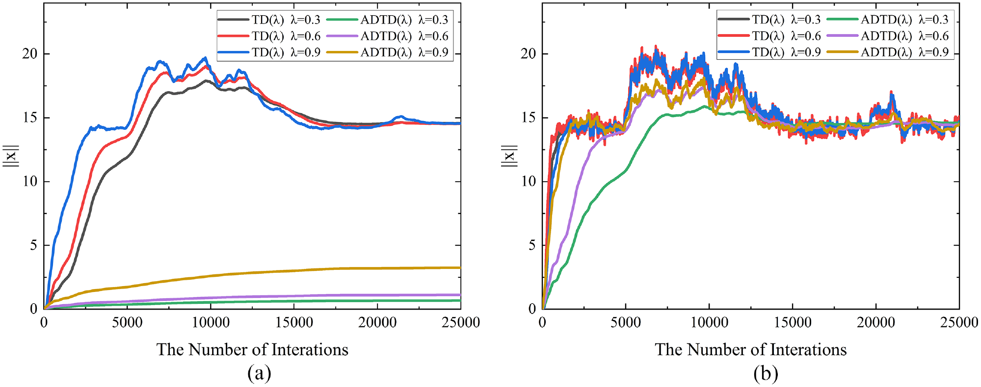
In this section, we verify the theoretical analysis results through a small ball experiment, which is similar to the experiment in Lin and Ling ³⁸ and Lowe et al. ³⁹ The agent interacts with the environment and the goal is to find the target node through continuous learning. The return obtained by the agent after each action is inversely proportional to the proximity of the target node, that is, the closer it is to the target node, the greater the return. The settings of experimental parameters are as follows: the discount factor $\gamma =0.95$ , and hyper-parameters ${\beta }_1=0.9$ , ${\beta }_2=0.999$ . We conducted four groups of comparative experiments, and the experimental results are shown in Figures 1–4. Next, we will introduce these figures separately.

Figure 1.

$\parallel x\parallel$ at the same initial step-size ${\alpha }_0=0.001$ and different $\lambda$ . (a) Decreasing step-size and (b) constant step-size

Figure 2.

$\parallel x\parallel$ at the same initial step-size ${\alpha }_0=0.0001$ and different $\lambda$ . (a) Decreasing step-size and (b) constant step-size

Figure 3.

$\parallel x\parallel$ at the same $\lambda =0.3$ and different initial step-size ${\alpha }_0$ . (a) Decreasing step-size and (b) constant step-size

Figure 4.

$\parallel x\parallel$ at the same $\lambda =0.9$ and different initial step-size ${\alpha }_0$ . (a) Decreasing step-size and (b) constant step-size

The initial step-size in Figures 1 and 2 is ${\alpha }_0=0.001$ and ${\alpha }_0=0.0001$ , respectively, and we compared the ordinary TD( $\lambda$ ) algorithm with the ADTD( $\lambda$ ) algorithm under the case of decreaing step-size (Figures 1(a) and 2(a)) and constant step-size (Figures 1(b) and 2(b)). The decreasing step-size is related to $t$ and the step-size will be smaller with the increase of time. Because our ordinate is $\parallel x\parallel$ , the change of parameter update of ADTD( $\lambda$ ) algorithm in the case of decreasing step-size will be smaller than that of constant step-size, and because ADTD( $\lambda$ ) algorithm combines AMSGrad algorithm, it will perform faster and more stably to ensure convergence. Experimental results show that our ADTD( $\lambda$ ) algorithm converges faster and is more stable in either case.

In Figure 3, we fix $\lambda =0.3$ and make the following experiments for decreasing step-size (Figure 3(a)) and constant step-size (Figure 3(b)). Overall, ADTD( $\lambda$ ) algorithm can always converge first at different initial step-size. In Figure 3(b), the parameter update adopts constant step-size, so the parameter update amplitude will increase as the ${\alpha }_0$ setting increases; it can also be seen that the greater the fluctuation of TD( $\lambda$ ) algorithm with the increase of $\alpha$ , the higher the curve for ADTD( $\lambda$ ) algorithm. Therefore, for constant step-size, the smaller the ${\alpha }_0$ , the more stable the curve. Although the convergence speed is sometimes similar in Figure 3(b), ADTD( $\lambda$ ) algorithm is more stable than TD( $\lambda$ ) algorithm because it uses adaptive algorithm.

In Figure 4, we fixed $\lambda =0.9$ and make the following experiments for decreasing step-size (Figure 4(a)) and constant step-size (Figure 4(b)). It should be clear that in Figure 4(b), when $\alpha =0.01$ , the algorithm cannot converge. The reason is that the larger the lambda and alpha, the worse the performance because $\lambda \in [0,1]$ . At this time, $\lambda =0.9$ , the scope of $\alpha$ is more strict.

Conclusion

We use reinforcement learning to solve the optimal routing problem based on wireless sensor networks. To this end, we propose an adaptive TD( $\lambda$ ) algorithm, referred to as ADTD( $\lambda$ ). We prove the non-asymptotic analysis of the adaptive TD( $\lambda$ ) algorithm under Markovian sampling. Furthermore, for ADTD( $\lambda$ ) with linear function approximation, we show that the algorithm can converge to the global optimal neighborhood in the case of constant step-size and decreasing step-size. However, under some parameter settings, the oscillation of the algorithm is large and the performance of the algorithm is not much different from that of the original $\mathrm{TD}(\lambda )$ algorithm; combining it with variance reduction technology will further improve the performance of the algorithm.