Sage Journals: Discover world-class research

Abstract

In wireless sensor networks, optimizing the network lifetime is an important issue. Most of the existing works define network lifetime as the time when the first sensor node exhausts all of its energy. However, such time is not necessarily important. This is because when a sensor node dies, the whole network is likely to work properly. In this article, we first make an overall consideration of the demand of applications and define the network lifetime in three aspects. Then, we construct a performance evaluation framework for routing protocols. To achieve the optimization of network lifetime in all defined aspects, we propose a reinforcement-learning-based routing protocol. Reinforcement-learning-based routing protocol takes advantage of the intelligent algorithm of reinforcement learning to search for the optimal routing path for data transmission. In the definition of reward function, factors such as link distance, residual energy, and hop count to the sink are taken into account to cut down the total energy consumption, balance the energy consumption, and improve the packet delivery. Simulation results demonstrate that compared with energy-aware routing, BEER, Q-Routing, and MRL-SCSO, reinforcement-learning-based routing protocol optimizes the network lifetime in three aspects and improves the energy efficiency.

Keywords

Wireless sensor networks network lifetime reinforcement learning routing protocol reward function energy efficiency

Introduction

In wireless sensor networks (WSNs), each of the sensor nodes has limited energy supply, constrained computation, and communication ability. Therefore, network lifetime becomes the major concern in WSNs.^1–3 With regard to network lifetime, most of the current researches define it as the time when the first sensor node exhausts all of its energy. However, such time is not necessarily important. This is because when a sensor node dies, the whole network is likely to work properly. For most applications of WSNs, they are concerned about whether the network can provide an acceptable service, which may focus on the percent of alive nodes, the connectivity to the sink, or the status of packet delivery. Thus, we define network lifetime in three aspects that are related to the above factors.

To prolong the network lifetime of WSNs, researchers have proposed methods such as mobile sink,^4–6 cross-layer design,^7–9 MAC protocol,^10–12 and routing protocol.^13–19 In this article, we focus on the research of routing protocol. For the proposed routing protocols for WSNs, according to the network structure, they can be categorized into flat routing and hierarchical routing. Our work is aimed at designing flat routing. Flat routing is suitable for smaller networks. In addition, for large-scale networks, hierarchical routing also demands a flat routing algorithm for intra-cluster communication. Among all of the flat routing protocols, energy-aware routing (EAR)¹⁴ is one of the most typical protocols, and it has also been proved in the surveys^20,21 to have much stronger energy efficiency than other flat routing protocols. To avoid the problem of always using the minimum energy path, EAR maintains multiple paths between source node and destination node and selects one of the paths to transmit data in a probability. This protocol has been compared with directed diffusion (DD), and the experiment results show that EAR can provide an overall improvement of 21.5% energy saving and an increase of 44% in network lifetime which is defined as the time of first-node-death. EAR has its inherent advantages, but it only considers the energy consumption of communication when determining the path selection probability. An improved version of the EAR protocol is presented. Different from EAR, balanced energy efficient routing (BEER)¹⁵ not only considers the energy consumption of communication but also considers the residual energy of nodes and the number of paths including the forwarding node when choosing the routing path. Simulation results show that this protocol can further extend the death time of the first node. However, just as EAR, the flooding process in the setup phase and route maintenance phase will bring about much more additional overhead. In addition, in these two protocols, the data are transmitted in accordance with the established routing table. The routing table which has been built in advance cannot fully reflect the current network status.

In this article, we propose a reinforcement-learning-based routing (RLBR) protocol to solve the problems mentioned above and maximize the lifetime optimization of WSNs. Reinforcement learning (RL) is a sub-area of machine learning technique and deals with how an agent should take actions in an environment to maximize the long-term reward.^22,23 The RL algorithm has its inherent advantages and is well suitable for dealing with distributed problems.^24,25 In this algorithm, each possible action is assigned a Q-value which indicates the approximate goodness of the action.²⁶ In the learning process, according to the Q-value of each action, the agent selects one action. After executing one action, the agent receives a reward. Then, the reward is used to update the Q-value of the action. Over time the agent learns the real Q-value of each action. Since the RL algorithm can achieve optimal results at nearly no additional costs using distributed learning,²⁷ it is suitable for dealing with the routing issue of WSNs. RLBR, the proposed protocol, utilizes the RL algorithm to optimize network lifetime of WSNs in all defined aspects. In RLBR, the equivalent of an agent is a sensor node. When sensor node i generates or receives a data packet, the action of node i is to select one forwarding node j in the light of Q(i, j). Q(i, j) represents the estimated total reward from node i to the sink through node j. The key point here is to properly define the reward function in order to better update Q-values. The main contributions of our work are summarized as follows:

We make an overall consideration of the demand of applications and define the network lifetime of WSNs from these three aspects of the condition of alive nodes, the connectivity to the sink, and the status of packet delivery. Based on this, we further construct a performance evaluation framework for routing protocols of WSNs.

We propose an RL-based routing protocol to optimize the network lifetime of WSNs in all defined aspects. In this proposed protocol, the next forwarder is selected according to the historical learning information and the current estimation information, and the factors such as residual energy, link distance, and hop count are taken into account to learn the best paths. Such a way can make sensor nodes keeping better connectivity to the sink, balance the energy consumption among sensor nodes, decrease the total energy consumption, and increase the packet delivery.

We take schemes such as data packet carrying feedback and transmit power adjusting to further decrease the total energy consumption and improve the energy efficiency.

The rest of the article is organized as follows. In section “Related works,” we introduce the related works. In section “Performance evaluation framework for routing protocols in WSNs,” we discuss the definition of network lifetime and construct a performance evaluation framework for routing protocols. Then, in section “Proposed protocol: RLBR,” we detail the proposed protocol. In section “Performance evaluation,” we take simulation experiments to validate the performance of the proposed protocol. Finally, we conclude the article in section “Conclusion.”

Related works

In recent years, the machine learning technique has gained much attention. RL is a sub-area of machine learning, and it attempts to use computer programs to generate patterns or rules from large data sets. In the RL algorithm, the agent selects one action according to the patterns or rules and receives a reward from the environment. Then, the reward is used to update the patterns or rules. By such a learning process, the optimal results can be achieved. Due to the characteristics of RL, it is very suitable to deal with the distributed problems. Accordingly, some researchers use RL algorithm to solve the routing problem of WSNs. In this section, we will introduce the RL-based routing protocols in WSNs.

JA Boyan and ML Littman²⁸ proposed a basic Q-learning protocol “Q-Routing.” This protocol aims at increasing the rate of packet delivery and takes the minimal delivery time into account to learn the best paths. For each node, its each neighbor is assigned a Q-value. The Q-value of one neighbor indicates the evaluated time spent on the packet delivery from the current node to the sink node through this neighbor. Experimental results show that Q-Routing is able to discover efficient routing policies in a dynamically changing network without knowing the network topology and traffic patterns in advance. P Wang and T Wang²⁹ applied a model-free learning algorithm “Least squares policy iteration (LSPI)” to learn an optimal routing strategy for WSNs and proposed the routing scheme “Adaptive routing (AdaR).” Different from Q-Routing which directly evaluates the optimal action-value function, AdaR approximates the Q-values Q^π for a given policy π with a parametric function, and considers factors such as hop count, residual energy, aggregated ratio, and link reliability. AdaR has been proved to gain a significant improvement in terms of convergence speed and sensitivity to the initial parameters over the basic Q-learning algorithm. Adaptive tree protocol (ATP) was proposed by Y Zhang and QF Huang.³⁰ The main idea of ATP is to use a type of reinforcement-learning-based meta-routing strategy for the constraint-based routing. The reinforcement-learning-based meta-routing strategy consists of three phases—initialization phase, forwarding phase, and confirmation phase—and learning happens in all phases. Based on this RL strategy, a spanning tree is constructed at initialization, but automatically maintained during the routing process. Simulation results show that ATP is robust for unpredictable link failures and mobile sinks.

In addition, there are some RL-based routing protocols for specific scenarios. A Forster and AL Murphy³¹ considered the multi-sink scenario and designed an energy-aware multicast routing protocol “Feedback routing for optimizing multiple sinks (FROMS).” FROMS attempts to minimize the energy dissipation while simultaneously delivering packets to multiple sinks. In FROMS, each node working as an agent learns the best hop costs to any combination of sinks. In the initialization phase, each sink broadcasts an announcement, and the hop counts of nodes to each sink are known. According to the information of hop counts, the initial Q-values of actions are estimated. In the data transmission phase, each node learns the real Q-values of the shared paths in the network. Simulation results show that FROMS can decrease the routing cost and also perform well in case of node failure and sink mobility. QELAR, presented by TS Hu and YS Fei,³² is an adaptive energy-aware distributed routing protocol for underwater wireless sensor networks (UWSNs). This protocol makes use of the RL technique to learn the environment effectively to better adapt to the dynamic topology of UWSNs. In the reward function, the residual energy of each node and the energy distribution among a group of nodes are considered to balance the energy consumption. In addition, the mechanism of detecting transmission failure is adopted to sense failure and update the corresponding Q-values.

In recent years, some researchers still use RL to solve the routing problems of WSNs. MA Razzaque et al.³³ provided a distributed adaptive cooperative routing (DACR) protocol. In the DACR protocol, a lightweight RL method is used to update the routing strategy. In the learning process, the knowledge on reliability and delay is taken into account to determine the reward value. FTIEE, a hierarchical RL-based routing protocol, is proposed by F Kiani et al.³⁴ to prolong the network lifetime of WSNs. In the first step of the protocol, a new clustering method is applied to the network. The size of the clusters increases with increasing distance to the sink, and the RL technique is used to choose cluster heads. Then, the Q-value parameter of RL is used to transmit data. Multi-agent reinforcement learning-based self-configuration and self-optimization (MRL-SCSO), proposed by AP Renold and S Chandrakala,³⁵ is a multi-agent reinforcement-learning-based self-configuration and self-optimization protocol for unattended WSNs. In this protocol, these factors of residual energy and buffer length are considered to define the reward function, and the neighbor with the maximum reward value is selected as the next forwarder. In addition, the sleep scheduling scheme is used to decrease the energy consumption. Compared with collect tree protocol (CTP), MRL-SCSO provides an increased lifetime which is defined as the time when the first node dies.

Our work differs from the previous works. Table 1 lists the main differences. In our work, factors such as residual energy, link distance, and hop count are considered to learn the best paths, and schemes such as data packet carrying feedback and transmit power adjusting are taken. Our goal is to optimize the network lifetime in all defined aspects and improve the energy efficiency.

Table 1.

Differences between our work and the previous works.

Routing protocols	Main characteristics
Q-Routing	Considering the minimal delivery time to learn the best paths.
AdaR	Considering residual energy, hop count, aggregated ratio, and link reliability to learn an optimal routing strategy.
ATP	Considering metrics for energy-aware load balancing and congestion-aware routing to build an adaptive spanning tree.
FROMS	Considering hop costs to learn the best paths to multiple sinks.
QELAR	Considering residual energy and energy distribution among a group of nodes to learn the best paths.
DACR	Considering the knowledge on reliability and delay to learn the best paths.
FTIEE	Dividing nodes into clusters with different sizes and using RL to choose cluster heads;Taking the data retransmission scheme.
MRL-SCSO	Considering residual energy and buffer length to learn the best paths;Taking the sleep scheduling scheme.
RLBR	Considering the factors such as residual energy, link distance, and hop count to learn the best paths;Taking the schemes such as data packet carrying feedback and transmit power adjusting.

AdaR: adaptive routing; ATP: adaptive tree protocol; FROMS: feedback routing for optimizing multiple sinks; RLBR: reinforcement-learning-based routing protocol.

Performance evaluation framework for routing protocols in WSNs

For WSNs, on one hand, network lifetime is an important metric for the performance evaluation. With regard to this issue, the pivotal problem is the particular meaning of network lifetime. On the other hand, for energy-constrained networks such as WSNs, energy efficiency reveals the work efficiency. Figure 1 illustrates our performance evaluation framework for routing protocols in WSNs. We evaluate the performance of routing protocols in terms of network lifetime and energy efficiency. For network lifetime, we define it from three aspects of the condition of alive nodes, the connectivity to the sink, and the status of packet delivery. For energy efficiency, it is related to two factors of the number of packet delivery and the total energy consumption.

Figure 1.

Performance evaluation framework for routing protocols in WSNs.

Network lifetime

There are numerous publications having researched on the lifetime of WSNs. They define network lifetime as:

The time until the first sensor is drained of its energy;^36–39

The time until the first cluster head is drained of its energy;⁴⁰

The time there is a certain fraction of surviving nodes in the network;^41–43

The time until all nodes have been drained of their energy;⁴⁴

The time each target is covered by at least one node;⁴⁵

The time the whole area is covered by at least one node;⁴⁶

The number of successful data-gathering trips;^47,48

The number of total transmitted messages;⁴⁹

The time until connectivity or coverage is lost;⁵⁰

The time period during which the network continuously satisfies the application requirement.⁵¹

Although there are various versions about the definition of network lifetime, they are only based on one of the following factors: number of alive nodes, connectivity, coverage, or quality of service. For most routing protocols proposed for WSNs, the evaluation of network lifetime is always based on a particular definition, and the most usual one is the time until the first node is drained of its energy. However, such time is not necessarily important. This is because when a sensor node dies, the whole network is likely to work properly. Most applications of WSNs care about whether the network can provide an acceptable service, which is related to the condition of alive nodes, the connectivity to the sink, and the status of packet delivery. Thus, we do an overall consideration of the demand of applications and define the network lifetime in three aspects.

Definition 1

Network lifetime: It contains three aspects: (1) the time until the first dead node appears; (2) the time until the first isolated node appears; and (3) the time until the network cannot accomplish any packet delivery.

In the definition, an isolated node is a node that has energy but has no path to the sink. This means that all the neighbor nodes of the isolated node have died. The first and second aspects show the moments at which the condition of alive nodes and the connectivity to the sink are changed. The third aspect denotes the time when the whole network cannot work any more. When evaluating the performance of network lifetime, these three moments rather than just a single one need to be evaluated.

Energy efficiency

The performance of energy efficiency shows the work efficiency of WSNs. We define it as follows:

Definition 2

Energy efficiency: The number of packet delivery by consuming unit energy, which can be calculated by equation (1)

E = N / EC

(1)

where E denotes the energy efficiency, N is the number of packet delivery, and EC represents the total energy consumption.

At a certain point, the energy efficiency of the network is determined by the number of packet delivery and the total energy consumption at that moment.

Proposed protocol: RLBR

In WSNs, when a sensor node generates or receives a packet, it needs to send the packet to the sink node. If the sensor node cannot reach the sink node directly, it is necessary to select one of its neighbors to forward the packet. How to select neighbor nodes is a routing problem, and the routing problem can be considered as a Markov decision process (MDP). Such a problem can be solved by the algorithm of RL. An RL task is described as an MDP (S; A; P; R,^52–54 in which S denotes the set of possible states, A indicates the set of possible actions, P represents the probability of state transition, and R symbolizes the environmental reward). The RL algorithm consists of two main parts: agent and environment. An agent perceives the current state of the environment and selects an action based on the current policy. Once taking an action, the agent will receive a reward from the environment. According to the reward, the agent updates its policy. In our protocol, the algorithm of RL is used and the following measures are taken to achieve the desired routing performance:

In the definition of reward function, residual energy of sensor node and link distance between nodes are taken into account to balance the energy consumption and decrease the total energy consumption.

The hop count to the sink is also considered to define the reward function, which can reduce the delay and indirectly improve the packet delivery.

In the RL-based routing, each node does not need global network information but can still approximate to the global optimization without additional cost.

Once a packet is generated, the correlative nodes find a routing path to deliver the packet to the sink. Each node searches for the next forwarder according to the up-to-date status rather than depending on the built routing table. Thus, the routing process is in accordance with the current condition of the network.

With regard to this condition that a node cannot find a neighbor to forward the packet, RLBR adopts two schemes. If the node has enough energy to reach the sink, it will adjust its transmission power to directly send the packet to the sink. Such a way solves the issue which is analogous to the void problem in geographic routing. Otherwise, the packet is dropped and the node is regarded as an isolated one. An isolated node has energy but has no path to the sink. After that, the isolated node will not be considered in the choice of next forwarder. Accordingly, the efficiency of path selection is improved.

Packet structure

In our model, there are two types of packets: control packet and data packet.

In network initialization phase, control packets are flooded from the sink. The structure of control packet is shown in Figure 2. The fields of node id, location coordinate, residual energy, and hop count indicate the information of the previous forwarder.

Figure 2.

Structure of control packet.

In data communication phase, each sensor node sends a data packet to the sink every interval. The structure of data packet is defined in Figure 3. When a node hears a data packet, it first extracts the information of the previous forwarder including node id, location coordinate, residual energy, hop count to the sink, and Q-value. Among them, Q-value represents the current evaluation of the path quality from the previous forwarder to the sink. Then, if the field of next forwarder indicates that the current node is not the eligible one to forward the packet, it simply drops the packet. Otherwise, the node selects the next hop.

Figure 3.

Structure of data packet.

Energy model

The first-order radio model,¹⁶ a generally accepted energy model for WSNs, is used in RLBR. When a sensor node sends or receives a packet, its energy is lessened according to equation (2)

{\begin{matrix} E_{Tx} (k, d) = E_{elec} k + ε_{amp} k d^{m} \\ E_{Rx} (k) = E_{elec} k \end{matrix}

(2)

where k represents the length of a packet, d indicates the transmission distance, and E_Tx(k,d) and E_Rx(k) denote the energy consumption to transmit and receive a packet with the length of k bits to a distance of d. These three factors of m, E_elec, and ε_amp are constants. E_elec symbolizes the energy consumption for the transmitter or receiver circuitry to transmit or receive unit data, ε_amp represents the energy consumption for the transmitter amplifier to transmit unit data to unit distance, and m is an exponent of propagation attenuation. Referring to Heinzelman et al.,¹⁶E_elec = 50 nJ/bit, ε_amp = 100 pJ/bit/m², and m = 2 or 4.

Protocol operation

In RLBR, each sensor node is an agent. For any sensor node i, when it generates or receives a packet, the state of the packet is the sensor node i, and the action of the sensor node i is to select a neighbor node j as the forwarding node based on the current Q(i, j). Q(i, j) denotes the evaluation of the path quality from node i to the sink through node j. After determining the next forwarder, node i updates its own Q-value according to the corresponding Q(i, j) and puts its latest information into the packet header. Once sending the packet to the next forwarder, the previous node of node i can also overhear this packet, and the Q-value in this packet can be regarded as a feedback of node i to the previous node. For the previous node, the feedback can be used in the next round of data transmission. Through the constant learning, the estimated Q-value of each path is getting closer to the real value. As shown in Figure 4, RLBR works as follows.

Figure 4.

Flowchart of RLBR.

First, the network is initialized. During this phase, starting from the sink node, each node sends a control packet to its neighbor nodes. As shown in Figure 2, the sender’s location, residual energy, and hop count to sink node are included in the control packet. Once receiving a control packet, the node i extracts the sender’s information and calculates the Q-value of the sender according to equation (3). Then, the sender’s information is recorded in the neighbor table of node i. Before sending out the control packet, node i computes its hop count to the sink by equation (4) and puts its own information into the control packet

Q (s) = E (s) / h (s)

(3)

where E(s) is the current energy of the sender, and h(s) is the hop count from the sender to the sink

h (i) = h (s) + 1

(4)

where h(i) and h(s) represent the hop count to the sink from the node i and the sender, respectively.

Then, data packets are transmitted in the network. The structure of the data packet is shown in Figure 2. For each sensor node, when it receives or overhears a packet, it extracts the sender’s information and updates its neighbor table. If the current node is not the sensor node indicated by the field of Next Forwarder, it drops the packet. Otherwise, the current node will undertake the task of forwarding the packet. To forward the packet, the current node first looks up its neighbor table. If there is a record of the sink node in the neighbor table, the current node directly sends the packet to the sink. If not, the current node seeks candidate nodes that can be used as forwarders from its neighbor table. As a candidate neighbor node, it must meet the following conditions: (1) it is not an isolated node. That is, its Q-value is not equal to 0. It needs to be explained here, an isolated node means that the node has no forwarding node to reach sink. (2) The hop count to the sink is less than that of the current node to the sink. (3) Compared to the distance from the current node to the sink, the current node is closer to it. (4) It is closer to the sink than the current node to the sink.

If there is no neighbor node meeting the above conditions, the current node becomes an isolated node and marks its Q-value to 0. Next, two situations are considered. If the current node has enough energy to reach the sink, it adjusts the transmit power and directly sends the packet to the sink. This measure is to enable the node to make the last effort to send the packet so that the packet delivery is improved. Otherwise, the current node throws away the packet.

If there are multiple candidate neighbor nodes, the current node calculates the relevant Q-value of each one according to equation (5)

\begin{matrix} Q_{new} (cur, nbr) = \\ (1 - α) Q_{old} (cur, nbr) + α (R (cur, nbr) + Q (nbr)) \end{matrix}

(5)

where α symbolizes the learning rate, Q(cur,nbr) indicates the estimated quality of the path from the current node to the sink through a certain neighbor node, R(cur,nbr) represents the reward for the current node to send a packet to this neighbor node, and Q(nbr) denotes the quality of the path from this neighbor node to the sink. Q(nbr) can be obtained from the neighbor table, and R(cur,nbr) can be calculated by equation (6)

R (cur, nbr) = E (nbr) / (d^{n} (cur, nbr) \times h (nbr))

(6)

where E(nbr) and h(nbr) represent the residual energy of the neighbor node and the hop count from this neighbor node to the sink. Both of these can be obtained from the neighbor table. d(cur,nbr), as the distance between the current node and this neighbor node, can be computed according to equation (7). In addition, n is a constant and its value is shown in equation (8)

d (cur, nbr) = \sqrt{{(x (nbr) - x (cur))}^{2} + {(y (nbr) - y (cur))}^{2}}

(7)

where (x(cur), y(cur)) and (x(nbr), y(nbr)) are the location coordinates of the current node and the neighbor node

n = {\begin{matrix} 2 & d \leq d_{0} \\ 4 & otherwise \end{matrix}

(8)

where d₀ is a constant of distance threshold.

As equation (6) shows, the reward R(cur,nbr) is determined by three factors. In WSNs, for a sensor node, the more residual energy it has, the more tasks it can undertake. The less the hop count to the sink, the smaller the probability of packet loss. Therefore, in RLBR, the reward is proportional to the residual energy of the neighbor node and inversely proportional to the hop count of the neighbor node to the sink. Such a measure can balance the energy consumption of nodes in the network and improve the packet delivery. Besides, R(cur,nbr) is also determined by the distance between the current node and the neighbor node. If the distance is greater than the threshold d₀, R(cur,nbr) is inversely proportional to the four power of the distance. On the contrary, R(cur,nbr) is inversely proportional to the square of the distance. This is because that there is the same relationship between the energy consumption for transmitting data and the transmission distance, which is shown in equation (2). In this way, the shorter the distance between the current node and the neighbor node, the larger the reward for the current node to send a packet to this neighbor node. Then, the possibility of choosing this neighbor node as a forwarding node is greater. Consequently, the energy consumption for the current node to send a packet to the next forwarder is less. Thus, from a global perspective, this scheme can reduce the total energy consumption of data transmission in the network.

By the calculation of equation (5), the current node selects the candidate neighbor node with the maximal Q(cur,nbr) as the next forwarder and updates its own Q-value and hop count by equations (9) and (10)

Q (cur) = \max_{nbr \in N} Q (cur, nbr)

(9)

where N is the set of the candidate neighbor nodes of the current node, nbr is any of these nodes, and Q(cur) represents the Q-value of the current node. That is to say, the quality of the optimal path from the current node to the sink is equal to the maximal Q(cur,nbr)

h (cur) = h (nbr) + 1

(10)

where nbr is the node chosen as the next forwarder, and h(cur) and h(nbr) denote the hop count of the current node and the chosen node, respectively.

After that, the current node updates the packet header with its own information including node id, location coordinate, residual energy, hop count to the sink, and Q-value and then sends the packet to the next forwarder. The previous node can also overhear this packet, and the Q-value in this packet can be regarded as a feedback of the current node to the previous node. For the previous node, the feedback can be used in the next round of data transmission. Such a measure that the data packet carries the feedback can save energy.

Protocol operation sample

To explain the protocol operation more clearly, we give an example as follows. Figure 5 shows the network topology and the initial conditions of the example. For each node, the network topology in Figure 5 only shows its neighbor nodes that can be used as candidate nodes. After network initialization, node i₁ first collects data and sends it out. Next, node i₂ sends its collected data in the second round of data transmission. In the third round of data transmission, node i₁ sends its collected data again.

Figure 5.

Network topology and initial conditions of the example.

In RLBR, the main steps of data transmission are illustrated in Figures 6 –8. In the first round of data transmission, Table 2 is the neighbor table of node i₁, and Table 3 is the neighbor table of node j₂. In the second round of data transmission, Tables 4 and 5 are the neighbor tables of node i₂ and node j₃. Finally, Tables 6 and 7 are the neighbor tables of node i₁ and node j₂ in the third round of data transmission.

Figure 6.

The first round of data transmission in RLBR.

Figure 7.

The second round of data transmission in RLBR.

Figure 8.

The third round of data transmission in RLBR.

Table 2.

Neighbor table of node i₁ in the first round of data transmission in RLBR.

i ₁	j ₁	j ₂	j ₃
Location coordinate	(35, 10)	(55, 20)	(60, 15)
Residual energy	0.5	0.5	0.5
Hop count	4	2	3
Q-value	0.1250	0.2500	0.1667

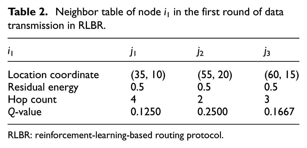
RLBR: reinforcement-learning-based routing protocol.

Table 3.

Neighbor table of node j₂ in the first round of data transmission in RLBR.

j ₂	k ₁	k ₂
Location coordinate	(40, 30)	(70, 45)
Residual energy	0.5	0.5
Hop count	1	1
Q-value	0.5000	0.5000

RLBR: reinforcement-learning-based routing protocol.

Table 4.

Neighbor table of node i₂ in the second round of data transmission in RLBR.

i ₂	j ₃	j ₄
Location coordinate	(60, 15)	(75, 10)
Residual energy	0.5	0.5
Hop count	3	4
Q-value	0.1667	0.1250

RLBR: reinforcement-learning-based routing protocol.

Table 5.

Neighbor table of node j₃ in the second round of data transmission in RLBR.

j ₃	j ₂	k ₃
Location coordinate	(55, 20)	(65, 30)
Residual energy	0.4999	0.5
Hop count	2	1
Q-value	0.2508	0.5000

RLBR: reinforcement-learning-based routing protocol.

Table 6.

Neighbor table of node i₁ in the third round of data transmission in RLBR.

i ₁	j ₁	j ₂	j ₃
Location coordinate	(35, 10)	(55, 20)	(60, 15)
Residual energy	0.5	0.4999	0.4999
Hop count	4	2	2
Q-value	0.1250	0.2508	0.2510

RLBR: reinforcement-learning-based routing protocol.

Table 7.

Neighbor table of node j₂ in the third round of data transmission in RLBR.

j ₂	k ₁	k ₂
Location coordinate	(40, 30)	(70, 45)
Residual energy	0.4999	0.5
Hop count	1	1
Q-value	0.4999	0.5000

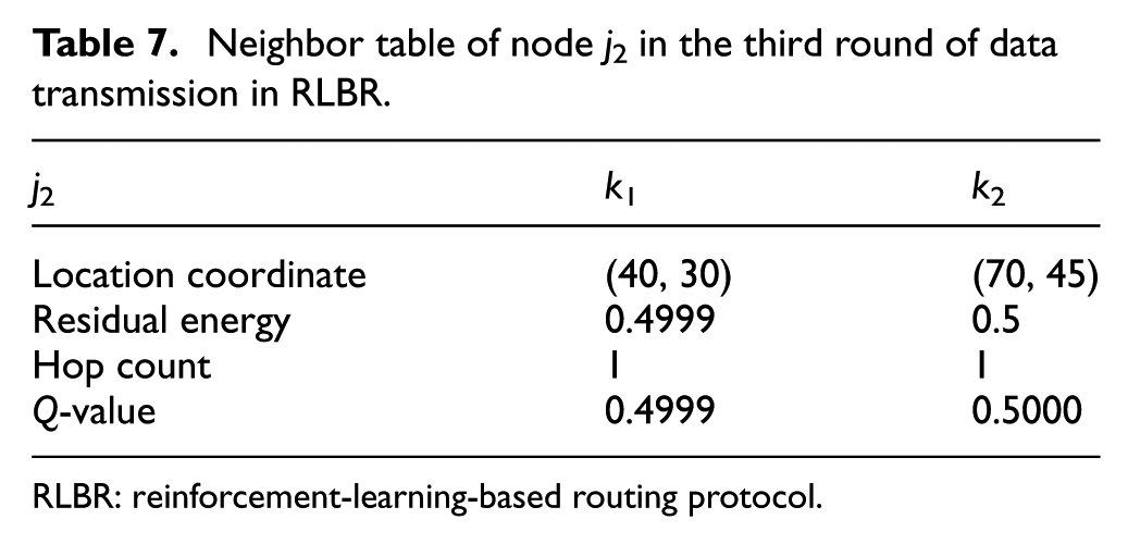
RLBR: reinforcement-learning-based routing protocol.

To show the differences between RLBR and other RL-based routing protocols, we select the most classical RL-based routing protocol “Q-Routing” as an example. Q-Routing considers the minimal delivery time to learn the best paths. In Q-Routing, the Q-value of each node is initialized to 0. In data transmission phase, according to the original definition, the Q-value is computed by equation (11). It should be noted that in order to compare the routing protocols under the same conditions, we do not consider the time in the queue in equation (11)

Δ Q (cur, nbr) = α (\overset{Q_{new} (cur, nbr)}{\overset{︷}{T (cur, nbr) + Q (nbr)}} - Q_{old} (cur, nbr))

(11)

After transformation, equation (11) is equivalent to equation (12)

\begin{matrix} Q_{new} (cur, nbr) = \\ (1 - α) Q_{old} (cur, nbr) + α (T (cur, nbr) + Q (nbr)) \end{matrix}

(12)

where α symbolizes the learning rate, Q(cur,nbr) indicates the minimal delivery time for the current node to send a packet to the sink through a certain neighbor node, T(cur,nbr) represents the time taken to transmit a packet from the current node to this neighbor node, and Q(nbr) denotes the minimal delivery time for this neighbor node to send a packet to the sink by multi-hop forwarding. T(cur,nbr) is mainly determined by link distance, and it can be computed by equation (13)

T (cur, nbr) = d (cur, nbr) / v

(13)

where d(cur,nbr) represents the link distance, and v stands for data transmission rate. Here, we assume that v = 1.

The current node selects the candidate node with the minimal Q(cur,nbr) as the next forwarder and updates its own Q-value by equation (14)

Q (cur) = \min_{nbr \in N} Q (cur, nbr)

(14)

where N is the set of the current node’s neighbor nodes.

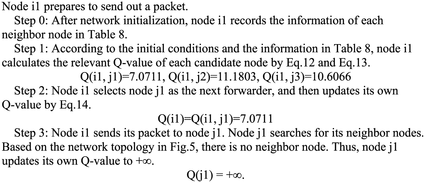
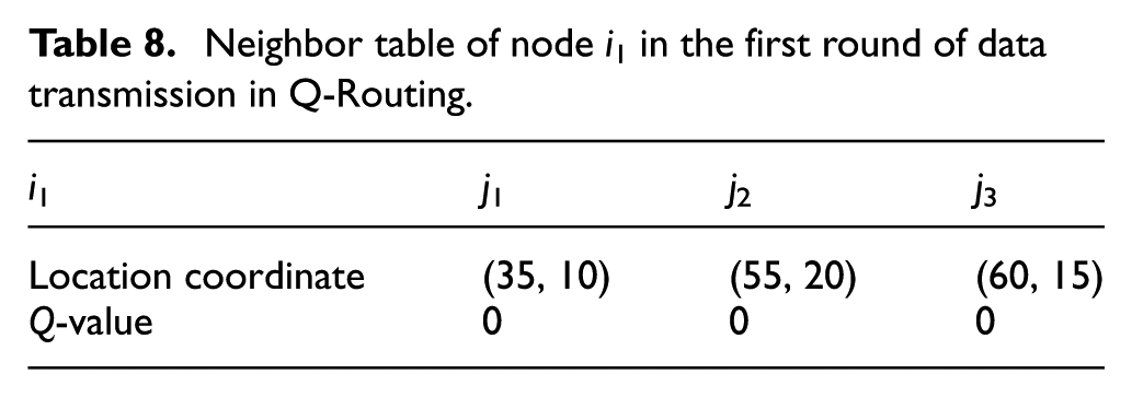
Based on the network topology and initial conditions in Figure 5, the data transmission processes in Q-Routing are shown in Figures 9 –11. In the first round of data transmission, the neighbor table of node i₁ is shown in Table 8. In the second round of data transmission, the neighbor table of node i₂ is shown in Table 9. And Tables 10 –12 show the neighbor tables of node i₁, node j₃, and node j₂ in the third round of data transmission.

Figure 9.

The first round of data transmission in Q-Routing.

Figure 10.

The second round of data transmission in Q-Routing.

Figure 11.

The third round of data transmission in Q-Routing.

Table 8.

Neighbor table of node i₁ in the first round of data transmission in Q-Routing.

i ₁	j ₁	j ₂	j ₃
Location coordinate	(35, 10)	(55, 20)	(60, 15)
Q-value	0	0	0

Table 9.

Neighbor table of node i₂ in the second round of data transmission in Q-Routing.

i ₂	j ₃	j ₄
Location coordinate	(60, 15)	(75, 10)
Q-value	0	0

Table 10.

Neighbor table of node i₁ in the third round of data transmission in Q-Routing.

i ₁	j ₁	j ₂	j ₃
Location coordinate	(35, 10)	(55, 20)	(60, 15)
Q-value	+∞	0	0

Table 11.

Neighbor table of node j₃ in the third round of data transmission in Q-Routing.

j ₃	j ₂	k ₃
Location coordinate	(55, 20)	(65, 30)
Q-value	0	0

Table 12.

Neighbor table of node j₂ in the third round of data transmission in Q-Routing.

j ₂	k ₁	k ₂
Location coordinate	(40, 30)	(70, 45)
Q-value	0	0

To sum up, Figures 12 and 13 illustrate the path selection results in RLBR and Q-Routing. In Q-Routing, the Q-value of each node is initialized to 0. Thus, at the beginning, the current node only considers the distance to the neighbor node to select the next forwarder. In this case, it is equivalent to using greedy algorithm to select routing path. After data transmission, sensor nodes update their Q-value by learning. Then, sensor nodes choose routing path from the perspective of global optimization. However, in RLBR, the Q-value of each node is initialized by residual energy and hop count to the sink. Therefore, RLBR can find a relatively optimal path in the initial phase. After multiple rounds of data transmission, on one hand, the energy of nodes will change more and more. On the other hand, due to the death of nodes, the network topology will also change more and more. Q-Routing only considers the minimal delivery time to learn the best paths, while RLBR considers factors such as residual energy, link distance, and hop count to the sink to learn the best paths. Thus, with the increase in the rounds of data transmission, the advantages of RLBR in path selection will become more and more obvious.

Figure 12.

Path selection results in RLBR: (a) the first round, (b) the second round, and (c) the third round.

Figure 13.

Path selection results in Q-Routing: (a) the first round, (b) the second round, and (c) the third round.

Protocol analysis

In this section, we list the optimization measures in RLBR and analyze the protocol performance, which reveals the contributions of RLBR. RLBR takes the following measures to optimize the performance:

Once a packet is generated, the correlative nodes find a routing path to deliver the packet to the sink. Each node searches for the next forwarder according to the up-to-date status rather than entirely depending on the routing table. That is to say, the routing process is in accordance with the current condition of the network. Such a way can make nodes keeping better connectivity to the sink.

In the process of data transmission, the current node chooses the next forwarder from the candidate nodes. As a candidate node, it must be closer to the sink than the current node to the sink. For example, if node A chooses node B as the next forwarder, and node B chooses node C as the next forwarder. Then, the distance from node A to the sink is greater than that from node B to the sink, and the distance from node B to the sink is greater than that from node C to the sink. For node C, it must select a node closer to sink as the next forwarder. Therefore, node C will not select nodes such as A and B to forward data. Thus, there is no routing loop in RLBR.

For each candidate node, the current node calculates its corresponding Q-value. As shown in equation (5), the Q-value is mainly influenced by the reward. It can be seen from equation (6) that the value of the reward is determined by link distance, hop count to the sink, and residual energy. For a candidate node, its corresponding reward is proportional to its residual energy. The more residual energy the candidate node has, the greater reward value the current node will get if sending a packet to this candidate node. Then, the possibility of choosing this candidate node as the next forwarder is larger. Such a measure can make sensor nodes consume energy more evenly.

The reward is also determined by the link distance. If the link distance is greater than the threshold, the reward is inversely proportional to the four power of the distance. Otherwise, the reward is inversely proportional to the square of the distance. That is to say, the shorter the link distance between the current node and the candidate node, the greater the possibility for selecting this candidate node as the next forwarder. According to the energy model of WSNs, the shorter the transmission distance, the less the energy consumption for transmitting data. Therefore, this scheme can decrease the total energy consumption.

In addition to residual energy and link distance, the reward is also affected by the hop count to the sink. The less the hop count from a candidate node to the sink, the greater the probability for this candidate node to be selected as the next forwarder. Such a way can lessen the probability of packet loss and quicken the packet delivery.

The scheme of data packet carrying feedback is taken in RLBR. When the current node sends the packet to the next forwarder, the previous node can also overhear a feedback. This feedback can be used to update the Q-value of the previous node in the next round of data transmission. By such a distributed learning, it is able to achieve optimal results at nearly no additional energy costs. This scheme can reduce the total energy consumption of the network to a certain extent.

With regard to this condition that a node cannot find a neighbor to forward the packet, two schemes are adopted in RLBR. If the node has enough energy to reach the sink, it will adjust its transmission power to directly send the packet to the sink. Otherwise, the packet is dropped and the node is regarded as an isolated one. An isolated node has energy but has no path to the sink. After that, the isolated node will not be considered in the choice of next forwarder. Accordingly, the efficiency of path selection is improved. These schemes can increase the packet delivery.

In WSNs, for a sensor node, the modules consuming energy include sensor module, processor module, and wireless communication module. However, in practical work, the energy consumption of a sensor node is mainly focused on the wireless communication module, and the energy consumption for sending data is the largest. Compared with the energy cost of sending data, the computation cost is negligible. For the whole network, if the total energy consumed by transmitting data is reduced and the energy consumption between nodes is more evenly, the time of the first dead node appearing will be postponed. Thus, the above measures 3, 4, and 6 can optimize the network lifetime in the first aspect. In addition, an isolated node means that the node is alive but the neighbor nodes are dead. If the protocol can make the nodes in the network consume energy more evenly or reduce the total energy consumption of data transmission, the time of the isolated node appearing can also be delayed. Therefore, due to the above measures 1, 3, 4, and 6, the second aspect of the network lifetime can be enhanced. For the third aspect of network lifetime, measures 5 and 7 can optimize the performance. Finally, since the above measures 4 and 6 can decrease the total energy consumption and measures 5 and 7 can improve the packet delivery, the performance of energy efficiency is optimized accordingly.

In summary, RLBR is different from the previous works. The main differences among RLBR, Q-Routing, and MRL-SCSO are shown in Table 13. For each routing protocol, Table 13 lists its main characteristics and the corresponding effects, with regard to the detailed contributions of RLBR, as mentioned above. In addition, the performances of RLBR, Q-Routing, and MRL-SCSO will be further compared and analyzed in section “Performance evaluation.”

Table 13.

The main differences among RLBR, Q-Routing, and MRL-SCSO.

Routing protocols	Characteristics	Effects
1. Q-Routing	1-1. Selecting next forwarder based on historical learning information and current estimation information;	1-1. Making nodes keeping better connectivity to the sink;
1. Q-Routing	1-2. Considering the minimal delivery time to learn the best paths.	1-2. Quickening the packet delivery.
2. MRL-SCSO	2-1. Selecting next forwarder based on current estimation information;	2-1. /
	2-2. Considering factors such as residual energy and buffer length to learn the best paths;	2-2. Balancing the energy consumption; reducing the packet loss;
	2-3. Taking the scheme of sleep scheduling.	2-3. Decreasing the energy consumption.
3. RLBR	3-1. Selecting next forwarder based on historical learning information and current estimation information;	3-1. Making nodes keeping better connectivity to the sink;
	3-2. Considering factors such as residual energy, link distance, and hop count to learn the best paths;	3-2. Balancing and decreasing the energy consumption; increasing the packet delivery;
	3-3. Taking the scheme of data packet carrying feedback;	3-3. No additional energy consumption;
	3-4. Taking two schemes to deal with the condition that a node cannot find a neighbor to forward the packet: if the node has enough energy to reach the sink, it will adjust its transmission power to directly send the packet to the sink. Otherwise, the node is marked as an isolated one, which will not be considered in the choice of next forwarder.	3-4. Increasing the packet delivery;Improving the efficiency of path selection.

RLBR: reinforcement-learning-based routing protocol.

Performance evaluation

In this section, we evaluate the performance of our proposed protocol RLBR in terms of the network lifetime which is defined in three aspects and the energy efficiency. We have implemented these protocols of EAR, BEER, Q-Routing, MRL-SCSO, and RLBR in NS2. EAR is used in our comparison due to its inherent advantages. It is a typical flat routing protocol and has been proved to have much stronger energy efficiency than other flat routing protocols. BEER is an improved version of EAR and has been validated to postpone the death of the first node. In addition, we also compare our protocol with other RL-based routing protocols. Among these RL-based routing protocols, Q-Routing is an early classical representative and MRL-SCSO is a recent representative. Thus, we select these four protocols as our comparison objects.

The simulation parameters are specified in Table 14. According to the parameters setup, 10 kinds of network topologies are randomly generated. Under each network topology, these four protocols are tested. The comparison results are shown as follows. It needs to be explained that the following results reveal the average situations.

Table 14.

Simulation parameters.

Parameter	Value
Number of sensor nodes	100
Number of sink node	1
Topological area	100 m × 100 m
Initial energy of sensor nodes	0.5 J
Sensor nodes deployment	Random
Sink node deployment	(50, 50)
Transmission radius	30 m
Packet generation rate	1 s
Data packet size	512 bits
Learning rate, a	0.5
Distance threshold, d₀	15 m

Network lifetime in the first aspect

First of all, we test the performance of network lifetime in the first aspect, which is defined as the time until the first dead node appears. Figure 14 illustrates the results of the percent of alive nodes over time. In EAR, BEER, Q-Routing, MRL-SCSO, and RLBR, the first node dies at about 50, 80, 30, 140, and 150 s, respectively. Clearly, compared to the other three protocols, RLBR extends the network lifetime. On average, RLBR yields 200%, 88%, 400%, and 7% longer lifetime over EAR, BEER, Q-Routing, and MRL-SCSO, respectively.

Figure 14.

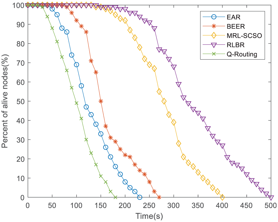
Percent of alive nodes over time.

As can be seen from Figure 14, Q-Routing has the shortest network lifetime. This is because it does not consider any energy-related factor to choose the routing path. In RLBR, once receiving or overhearing a packet, the sensor node selects one node as the next forwarder according to the Q-values of the candidate neighbors. After determining the next forwarder, the current node updates its own Q-value. When the current node sends the packet to the checked node, the previous node can also overhear a feedback and use it to update its Q-value in the next round of data transmission. By such a distributed learning, it is able to achieve optimal results at nearly no additional costs. But EAR and BEER have more additional spending since they need to build and maintain the routing table by periodically flooding.

In MRL-SCSO, the sleep scheduling scheme can decrease the energy consumption. However, in RLBR, the scheme of data packet carrying feedback can also save energy. Moreover, RLBR takes link distance into account to define the reward function, which can further cut down the energy consumption. In RLBR, if the link distance is greater than the threshold, the reward is inversely proportional to the four power of the link distance. Otherwise, the reward is inversely proportional to the square of the link distance. The result is that the shorter the link distance, the larger the reward for the current node to send a packet to this neighbor node. Then, the possibility of choosing this neighbor node as the next forwarder is greater. Accordingly, the energy consumption for the current node to send a packet to the next forwarder is less. From a global perspective, this scheme can reduce the total energy consumption of data transmission. In addition, in RLBR, the residual energy of node is also considered to define the reward, which can balance the energy consumption. Thus, RLBR can prolong the network lifetime in the first aspect.

Network lifetime in the second aspect

Then, we pay attention to the network lifetime in the second aspect, which is defined as the time until the first isolated node appears. Figure 15 reveals the comparison of connectivity to the sink. The experiment was implemented for 10 rounds. The vertical coordinate indicates the time of the first isolated node appearing in each round. An isolated node has energy but has no path to the sink. Such a node cannot send any packet to the sink. Thus, it is equivalent to an invalid node. It can be seen that RLBR gains a significant improvement of network lifetime in terms of the second definition over EAR, BEER, Q-Routing, and MRL-SCSO.

Figure 15.

Time of the first isolated node appearing in each round.

EAR and BEER select the next forwarder fully depending on the routing table, MRL-SCSO selects the next forwarder according to the current estimation information, and RLBR chooses the next forwarder according to the historical learning information and the current estimation information. The routing process in MRL-SCSO and RLBR is in accordance with the current condition of the network. Therefore, compared to EAR and BEER, MRL-SCSO and RLBR can make nodes keeping better connectivity to the sink. For Q-Routing, it also considers the historical learning information and the current estimation information to select the next forwarder. From this point of view, the connectivity performance of Q-Routing is better than that of EAR and BEER. However, the first dead node appears earliest in Q-Routing, which weakens the connectivity performance of Q-Routing. Thus, the performance of Q-Routing in the second aspect of network lifetime is slightly worse than that of EAR.

As for MRL-SCSO and RLBR, RLBR has the following advantages. First, in MRL-SCSO, the neighbor with the maximum reward value is selected as the next forwarder. That is to say, MRL-SCSO only considers the current estimation information to choose routing path, while RLBR considers the historical learning information and the current estimation information. Such a way in RLBR can provide better network connectivity. Second, an isolated node means that the node is alive but the neighbor nodes are dead. If the protocol can make the nodes in the network consume energy more evenly or reduce the total energy consumption of data transmission, the time of the isolated node appearing can be delayed. As discussed in section “Network lifetime in the first aspect,” the total energy consumption in RLBR is less than that in MRL-SCSO. Therefore, in the second aspect of network lifetime, the performance of RLBR is better than that of MRL-SCSO.

Network lifetime in the third aspect

For the third aspect of network lifetime, it is defined as the time until the network cannot accomplish any packet delivery. Figure 16 reflects the number of packet delivery over time. After 230, 270, 180, 400, and 500 s, the total number of packet delivery in EAR, BEER, Q-Routing, MRL-SCSO, and RLBR no longer changes. That is to say, at these times, the network can no longer complete any packet delivery. It is apparent that RLBR achieves longer lifetime over EAR, BEER, Q-Routing, and MRL-SCSO in the third aspect of network lifetime. In addition, as can be seen from Figure 16, although RLBR hands over fewer packets to the sink at the beginning, the superiority of RLBR is obvious at most of the time. After 110 s, RLBR delivers more packets than the other four protocols, and the gap is getting bigger and bigger. This is because RLBR needs to gradually learn from the environment. Initially, it evaluates the approximate goodness of each action. Afterward, it increasingly learns the real situation, which can be used to select the most appropriate path to transmit the packet.

Figure 16.

Number of packet delivery over time.

In Q-Routing, the minimal delivery time is taken into account to learn the best paths, which can quicken the packet delivery. Therefore, Q-Routing delivers the largest number of packets at the beginning. However, after 110 s, more than half of the nodes in Q-Routing exhaust their energy. Accordingly, the number of new delivered packets in Q-Routing decreases. In RLBR, when a node becomes an isolated node, the scheme of adjusting transmit power is used to let the node make the last effort to send the packet to the sink, which can improve the packet delivery to a certain extent. Besides, different from EAR, BEER, Q-Routing, and MRL-SCSO, RLBR also considers the hop count to the sink to search for the routing path. Under the similar condition of energy-related factors, it encourages nodes to select the next forwarder nearer to the sink, which can reduce packet loss and quicken packet delivery. Therefore, RLBR can improve the packet delivery.

Summary of network lifetime

Figure 17 sums up the comparative results of network lifetime in three aspects. In EAR, the first node dies at 50 s, the first isolated node appears at 90 s, and the network cannot accomplish any packet delivery at 230 s. These three moments in EAR can be marked as (50 s, 90 s, 230 s). In BEER, Q-Routing, MRL-SCSO, and RLBR, the three moments are (80 s, 190 s, 270 s), (30 s, 80 s, 180 s), (140 s, 310 s, 400 s), and (150 s, 350 s, 500 s), respectively. It can be seen that RLBR has obvious advantages in three aspects of network lifetime.

Figure 17.

Comparison of network lifetime in three aspects.

Energy efficiency

Finally, we test the performance of energy efficiency, which is defined as the number of packet delivery by consuming unit energy. Figure 18 shows the number of packet delivery over energy consumption. At first, in the case of consuming the same energy, MRL-SCSO and RLBR deliver less packets than EAR, BEER, and Q-Routing, which is due to the initial learning in MRL-SCSO and RLBR. Through continuous learning, the most appropriate path can be selected to transmit the packet, which will improve the packet delivery. Thus, the energy efficiency in MRL-SCSO and RLBR is gradually higher than EAR, BEER, and Q-Routing. For MRL-SCSO and RLBR, the energy efficiency of the latter is still higher than that of the former. Moreover, as the energy consumption increases, the difference of packet delivery between RLBR and the other four protocols is more obvious.

Figure 18.

Number of packet delivery over energy consumption.

The predominance of RLBR is caused by its characteristics. For the energy consumption, first, when there is data needing to be transmitted, RLBR makes use of RL to compute and select the optimum routing path at nearly no additional costs. But in EAR and BEER, because of building and maintaining routing tables, there is extra energy overhead. Second, the reward in RLBR is influenced by the distance between the current node and the neighbor node. If the distance is greater than the threshold, the reward is inversely proportional to the four power of the distance. Otherwise, the reward is inversely proportional to the square of the distance. That is to say, the shorter the distance between the current node and the neighbor node, the larger the possibility for choosing this neighbor node as a forwarding node. Consequently, the energy consumption for the current node to send a packet to the next forwarder is less. This scheme can reduce the total energy consumption of data transmission in the network. Finally, in RLBR, the scheme of data packet carrying feedback can further save energy. For the packet delivery, RLBR considers the hop count to the sink to define the reward function to encourage nodes to select the next forwarder nearer to the sink. Such a way quickens the packet delivery and decreases packet loss and ultimately achieves an increase of packet delivery. In addition, RLBR takes the scheme of adjusting transmit power to let the node make the last effort to send the packet to the sink, which can improve the packet delivery to a certain extent. Therefore, RLBR can enhance the energy efficiency. For the applications of WSNs, RLBR can offer a better service with less cost.

Conclusion

Network lifetime is an important performance for WSNs. In this article, we have first defined the network lifetime of WSNs in three aspects and constructed a performance evaluation framework for routing protocols. Then, we have proposed an RL-based routing protocol for WSNs. RLBR makes uses of the superiority of RL to achieve the global optimization without additional cost. Moreover, it considers these factors of link distance, residual energy, and hop count to define the reward function and takes schemes such as data packet carrying feedback and adjusting transmit power to decrease the total energy consumption, balance the energy consumption, and improve the packet delivery. This protocol aims at enhancing the network lifetime of WSNs in all defined aspects and meeting the demand of such applications which are concerned about whether the network can provide an acceptable service. Although RLBR is a flat routing protocol, it can also be applied to the large-scale WSNs. In such networks, RLBR is able to handle the routing issue inside each cluster or among cluster heads. We have validated the performance of RLBR in NS2. RLBR shows superior performance over EAR, BEER, Q-Routing, and MRL-SCSO in terms of the percent of alive nodes, the connectivity to the sink, the number of packet delivery, and the energy efficiency. In future, we intend to test this protocol under real WSN environments like test-bed or deployments.

Footnotes

Handling Editor: Seokcheon Lee

Declaration of conflicting interests

The author(s) declared no potential conflicts of interest with respect to the research, authorship, and/or publication of this article.

Funding

The author(s) disclosed receipt of the following financial support for the research, authorship, and/or publication of this article: This work was supported by the Fundamental Research Funds for the Central Universities (Grant No. 2232015D3-29), the National Natural Science Foundation of China (Grant No. 61772128), and the Shanghai Municipal Natural Science Foundation (Grant No. 14ZR1400900).

ORCID iD

Wenjing Guo

References

Rault

Bouabdallah

Challal

Energy efficiency in wireless sensor networks: a top-down survey. Comput Netw 2014; 67(8): 104–122.

Yadav

RS.

A review on energy efficient protocols in wireless sensor networks. Wirel Netw 2016; 22(1): 335–350.

Halawani

Khan

AW.

Sensors lifetime enhancement techniques in wireless sensor networks—a survey. J Comput 2010; 2(5): 34–47.

Yun

Xia

Maximizing the lifetime of wireless sensor networks with mobile sink in delay-tolerant applications. IEEE T Mobile Comput 2010; 9(9): 1308–1318.

Kaswan

Nitesh

Jana

PK.

Energy efficient path selection for mobile sink and data gathering in wireless sensor networks. Int J Electron Comm 2017; 73: 110–118.

Yarinezhad

Sarabi

Reducing delay and energy consumption in wireless sensor networks by making virtual grid infrastructure and using mobile sink. Int J Electron Comm 2018; 84: 144–152.

Madan

Cui

Lall

et al . Cross-layer design for lifetime maximization in interference-limited wireless sensor networks. IEEE T Wirel Commun 2006; 5(11): 3142–3152.

Wang

Yang

et al . Network lifetime maximization with cross-layer design in wireless sensor networks. IEEE T Wirel Commun 2008; 7(10): 3759–3768.

Yetgin

Cheung

KTK

El-Hajjar

et al . Cross-layer network lifetime maximization in interference-limited WSNs. IEEE T Veh Technol 2015; 64(8): 3795–3803.

10.

Jha

Pandey

Pal

et al . An energy-efficient multi-layer MAC (ML-MAC) protocol for wireless sensor networks. Int J Electron Commun 2011; 65(3): 209–216.

11.

Dinh

Kim

et al . L-MAC: a wake-up time self-learning MAC protocol for wireless sensor networks. Comput Netw 2016; 105: 33–46.

12.

Dong

FQ.

A prediction-based asynchronous MAC protocol for heavy traffic load in wireless sensor networks. Int J Electron Commun 2017; 82: 241–250.

13.

Jain

Betweenness centrality based connectivity aware routing algorithm for prolonging network lifetime in wireless sensor networks. Wirel Netw 2016; 22(5): 1605–1624.

14.

Shah

Rabaey

. Energy aware routing for low energy ad hoc sensor networks. In: Proceedings of the IEEE wireless communications and networking conference, Orlando, FL, 17–21 March 2002, pp.350–355. New York: IEEE.

15.

Yessad

Tazarart

Bakli

et al . Balanced energy efficient routing protocol for WSN. In: Proceedings of the international conference on communications and information technology, Hammamet, Tunisia, 26–28 June 2012, pp.326–330. New York: IEEE.

16.

Heinzelman

Chandrakasan

Balakrishnan

. Energy-efficient communication protocol for wireless microsensor networks. In: Proceedings of the 33rd annual Hawaii international conference on system sciences, Maui, HI, 7 January 2000, pp.1–10. New York: IEEE.

17.

Sabet

Naji

HR.

A decentralized energy efficient hierarchical cluster-based routing algorithm for wireless sensor networks. Int J Electron Commun 2015; 69(5): 790–799.

18.

Pazzi

Boukerche

Grande

RED

et al . A clustered trail-based data dissemination protocol for improving the lifetime of duty cycle enabled wireless sensor networks. Wirel Netw 2017; 23(1): 177–192.

19.

Liu

Chang

Energy-efficient data sensing and routing in unreliable energy-harvesting wireless sensor network. Wirel Netw 2018; 24(2): 611–625.

20.

Zungeru

Ang

Seng

KP.

Classical and swarm intelligence based routing protocols for wireless sensor networks: a survey and comparison. J Netw Comput Appl 2012; 35(5): 1508–1536.

21.

Guo

Zhang

A survey on intelligent routing protocols in wireless sensor networks. J Netw Comput Appl 2014; 38(1): 185–201.

22.

Kaelbling

Littman

Moore

AW.

Reinforcement learning: a survey. J Artif Intell Res 1996; 4(1): 237–285.

23.

Littman

ML.

Reinforcement learning improves behaviour from evaluative feedback. Nature 2015; 521(7553): 445–451.

24.

Kordafshari

Pourkabirian

Meybodi

et al . Distributed QoS routing algorithm in large scale wireless sensor networks. In: Proceedings of the 2012 IEEE international symposium on industrial electronics, Hangzhou, China, 28–31 May 2012, pp.826–830. New York: IEEE.

25.

Al-Rawi

HAA

Yau

KLA.

Application of reinforcement learning to routing in distributed wireless networks: a review. Artif Intell Rev 2015; 43(3): 381–416.

26.

Lin

Schaar

MVD

. Autonomic and distributed joint routing and power control for delay-sensitive applications in multi-hop wireless networks. IEEE T Wirel Commun 2011; 10(1): 102–113.

27.

Kulkarni

Forster

Venayagamoorthy

GK.

Computational intelligence in wireless sensor networks: a survey. IEEE Commun Surv Tut 2011; 13(1): 68–96.

28.

Boyan

Littman

ML.

Packet routing in dynamically changing networks: a reinforcement learning approach. In: Proceedings of the international conference on neural information processing systems, Denver, CO, 29 November–2 December 1993, pp.671–678. New York: IEEE.

29.

Wang

. Adaptive routing for sensor networks using reinforcement learning. In: Proceedings of the IEEE international conference on computer & information technology, Seoul, South Korea, 20–22 September 2006, pp.219–224. New York: IEEE.

30.

Zhang

Huang

QF.

A learning-based adaptive routing tree for wireless sensor networks. J Commun 2006; 1(2): 1–10.

31.

Forster

Murphy

. FROMS: feedback routing for optimizing multiple sinks in WSN with reinforcement learning. In: Proceedings of the international conference on intelligent sensors, Melbourne, QLD, Australia, 3–6 December 2007, pp.371–376. New York: IEEE.

32.

Fei

YS.

QELAR: a machine-learning-based adaptive routing protocol for energy-efficient and lifetime-extended underwater sensor networks. IEEE T Mobile Comput 2010; 9(6): 796–809.

33.

Razzaque

Ahmed

MHU

Hong

et al . QoS-aware distributed adaptive cooperative routing in wireless sensor networks. Ad Hoc Netw 2014; 19(8): 28–42.

34.

Kiani

Amiri

Zamani

et al . Efficient intelligent energy routing protocol in wireless sensor networks. Int J Distrib Sens N 2015; 2015: 5–27.

35.

Renold

Chandrakala

MRL-SCSO: multi-agent reinforcement learning-based self-configuration and self-optimization protocol for unattended wireless sensor networks. Wirel Pers Commun 2017; 96: 5061–5079.

36.

Tian

Shen

Sang

YP.

Maximizing network lifetime in wireless sensor networks with regular topologies. J Supercomp 2014; 69(2): 512–527.

37.

Guo

Yan

Gan

et al . An intelligent routing algorithm in wireless sensor networks based on reinforcement learning. Appl Mech Mater 2014; 678: 487–493.

38.

Mohajerani

Gharavian

An ant colony optimization based routing algorithm for extending network lifetime in wireless sensor networks. Wirel Netw 2016; 22(8): 2637–2647.

39.

Guo

Zhang

Routing between nodes and multiple gateways in wireless mesh sensor network. J Circuit Syst Comp 2011; 20(8): 1477–1503.

40.

Soro

Heinzelman

. Prolonging the lifetime of wireless sensor networks via unequal clustering. In: Proceedings of the 19th IEEE international parallel and distributed processing symposium, Denver, CO, 4–8 April 2005, pp.1–8. New York: IEEE.

41.

Duarte-Melo

Liu

. Analysis of energy consumption and lifetime of heterogeneous wireless sensor networks. In: Proceedings of GLOBECOM2002, Taipei, Taiwan, 17–21 November 2002, pp.1–6. New York: IEEE.

42.

Cerpa

Estrin

ASCENT: adaptive self-configuring sensor networks topologies. IEEE T Mobile Comput 2004; 3(3): 272–285.

43.

Tekkalmaz

Korpeoglu

Distributed power-source-aware routing in wireless sensor networks. Wirel Netw 2016; 22(4): 1381–1399.

44.

Tian

Georganas

. A coverage-preserving node scheduling scheme for large wireless sensor networks. In: Proceedings of the 1st ACM international workshop on wireless sensor networks and applications, Atlanta, GA, 28 September 2002, pp.32–41. New York: IEEE.

45.

Cardei

Thai

et al . Energy-efficient target coverage in wireless sensor networks. In: Proceedings of INFOCOM2005, Miami, FL, 13–17 March 2005, pp.1976–1984. New York: IEEE.

46.

Bhardwaj

Chandrakasan

. Bounding the lifetime of sensor networks via optimal role assignments. In: Proceedings of INFOCOM 2002, New York, NY, 23–27 June 2002, pp.1587–1596. New York: IEEE.

47.

Mhatre

Rosenberg

Kofman

et al . A minimum cost heterogeneous sensor network with a lifetime constraint. IEEE T Mobile Comput 2005; 4(1): 4–15.

48.

Olariu

Stojmenovic

. Design guidelines for maximizing lifetime and avoiding energy holes in sensor networks with uniform distribution and uniform reporting. In: Proceedings of INFOCOM 2006, Barcelona, 23–29 April 2006, pp.1–12. New York: IEEE.

49.

Baydere

Safkan

Durmaz

Lifetime analysis of reliable wireless sensor networks. IEICE T Commun 2005; E88-B(6): 2465–2472.

50.

Sha

Shi

Modeling the lifetime of wireless sensor networks. Sensor Lett 2005; 3(2): 126–135.

51.

Kumar

Arora

Lai

. On the lifetime analysis of always-on wireless sensor network applications. In: Proceedings of the IEEE international conference on mobile ad-hoc and sensor systems, Washington, DC, 7 November 2005, pp.186–188. New York: IEEE.

52.

Naputta

Usaha

RL-based routing in biomedical mobile wireless sensor networks using trust and reputation. In: Proceedings of the 2012 international symposium on wireless communication systems, Paris, 28–31 August 2012, pp.521–525. New York: IEEE.

53.

Yau

KLA

Goh

Chieng

et al . Application of reinforcement learning to wireless sensor networks: models and algorithms. Computing 2015; 97(11): 1045–1075.

54.

Chen

Zhao

A reinforcement learning-based sleep scheduling algorithm for desired area coverage in solar-powered wireless sensor networks. IEEE Sens J 2016; 16(8): 2763–2774.

Optimizing the lifetime of wireless sensor networks via reinforcement-learning-based routing

Abstract

Keywords

Introduction

Related works

Performance evaluation framework for routing protocols in WSNs

Network lifetime

Definition 1

Energy efficiency

Definition 2

Proposed protocol: RLBR

Packet structure

Energy model

Protocol operation

Protocol operation sample

Protocol analysis

Performance evaluation

Network lifetime in the first aspect

Network lifetime in the second aspect

Network lifetime in the third aspect

Summary of network lifetime

Energy efficiency

Conclusion

Footnotes

Declaration of conflicting interests

Funding

ORCID iD

References