Sage Journals: Discover world-class research

Abstract

Load balancing is of great significance to extend the longevity of wireless sensor networks, due to the inherent imbalanced energy overhead in such networks. However, existing solutions cannot balance the load distribution in partially disconnected wireless sensor networks. For example, if a network is partitioned into several segments with different area sizes, some areas have much more traffic load than other areas. In this article, we propose a load-balanced routing scheme, which aims to balance energy consumption within each segment and among different segments. First, we adopt unequal transmission distances to build initial routing for intrasegment load balancing. Second, we adopt the genetic algorithm to build extra routing between different segments for intersegment load balancing. The unique character of our work is twofold. On one hand, we investigate partitioned wireless sensor networks where there are several isolated segments. On the other hand, we pursue load balancing from a global perspective rather than from a local one. Some simulations verify the effectiveness and the advantages of our scheme in terms of extra deployment cost, system longevity, and load balancing degree.

Keywords

Wireless sensor networks routing control intelligent computing load balancing genetic algorithm network lifetime

Introduction

Wireless sensor networks (WSNs) have become significant parts of the Internet of Things (IoT).^1,2 In general, a WSN is composed of a static sink and a lot of sensor nodes. A sensor node has limited battery capacity, and the batter is inconvenient to be replaced in most cases. Thus, energy saving must be considered for network lifetime maximization in WSNs. Furthermore, in most cases, WSNs adopt the many-to-one data collection pattern, which easily results in imbalanced energy overhead throughout the network. In severe cases, it will cause the premature death of the network.^3,4 Although wireless charging is an alternative solution to the energy limitation problem,^5,6 it is impractical in some environments. Therefore, load balancing still plays a key role in maintaining the long-term operation of such networks.

Load balancing has attracted wide interest in the study field of WSNs. Some researchers have provided three types of load-balancing strategies.⁷ The first type is hybrid transmission, such as Wang and colleagues,^8,9 in which sensor nodes have two data transmitting modes: (1) single-hop (SH) transmission, in which every node sends data to the sink by an one-hop way and does not need any relay node; and (2) multiple-hop (MH) transmission, in which most packets are sent to the destination by a relay way, that is, at least two hops of data delivery. The second type is power control, such as Zhang et al.,¹⁰ Kavitha et al.,¹¹ and Lai et al.,¹² in which sensor nodes with less data delivery tasks use shorter communication range while the reverse is performed for those with more data delivery tasks. The third type is multifactor routing, such as Liu et al.,¹³ Peng et al.,¹⁴ and Qin et al.,¹⁵ in which data delivery paths are determined according to some key factors, for example, the remaining energy of nodes, the distance between two nodes, and the density distribution of nodes.

The above load-balancing strategies can alleviate energy holes, but they have very limited effect on the improvement of network performance in some scenarios. For example, if the network is partitioned into several isolated parts, the above load balancing strategies are only confined in each part, and the load balancing among different parts cannot be performed.^16,17 This is because data transmission has limited distance, and this cannot adjust the energy consumption among different parts. Therefore, we need to find another solution to the load balancing issue among different isolated parts of the network.^18,19

The major contributions of this article are outlined as follows:

We design a solution to load balancing problem for a new type of network: partially disconnected WSNs. In such a network, some areas cannot communicate with each other by straight-line one-hop or multihop manner. The proposed solution consists of two kinds of load balancing methods: local load balancing within each segment and global load balancing among different segments.

We present an intrasegment routing mechanism, in which we adopt unequal transmission distances to build initial routing for intrasegment load balancing. This routing is based on a basic transmission distance which is derived to achieve energy consumption balancing for all nodes of the same segment. Multiple factors are used to select relay nodes of intrasegment routing: the basic transmission distance, the data traffic, and the residual energy.

We present an intersegment routing mechanism, in which creates extra routing between different segments for intersegment load balancing. This is achieved by the genetic algorithm, in which several nodes from one segment to another one formulate a chromosome. Two kinds of selection operation are used to complete the genetic algorithm: intrasegment crossover operation and intersegment crossover operation.

The rest of this article is organized in the following way. Existing load balancing routing methods are summarized in Section II. The system model, energy dissipation model, and the addressed problem are described in Section III. Section IV describes the details of our load-balanced routing protocol. Section V shows the simulations to verify the effectiveness and advantages of our proposed protocol. Finally, Section VI draws a conclusion.

Related works

In WSNs, routing is a basic task and it determines multiple aspects of the network performance.^20–22 In the past, many researchers studied this topic and proposed lots of load-balanced routing strategies in the literature. These strategies are categorized into three kinds, which are described latter. Clustering is a main concern in most load balancing methods; we focus on transmission local and global load balancing.

Mixed routing

The mixed routing means that all sensor nodes utilize two kinds of transmission patterns: SH and MH. Liang et al.²³ designed a hybrid routing mechanism for balancing energy dissipation of different nodes. In the SH pattern, data packets are sent to the destination by an one-hop manner, and accordingly the nodes with longer distances to the sink have more energy dissipation. In the MH pattern, data packets are sent to the destination through a multiple-hop pattern, so the nodes with shorter distances to the sink have more data delivery tasks. Wang et al.²⁴ also investigated the ring-shaped WSNs, and designed the transmission distances of the MH manner on the basis of two aspects: the width of the ring and the distance of the hop. Yang et al.²⁵ studied the corona WSNs, and regarded the load balancing issue as a data allocation problem by a hybrid transmission way. Sensor nodes in different areas use different ratio of the SH mode and the MH mode for load balancing. Teng et al.²⁶ regarded the communication distance adjustment as a 0-1 assignment problem, and put forward a dynamic programming approach to solve it. The communication distances of nodes are achieved on the basis of the nodes’ remaining energy. Liu et al.²⁷ designed a data aggregation tree with a bound of network lifespan. Nodes adopt adjustable transmission power, and the bound contains a term which is proportional to the difference of energy. In the mixed routing, the direct data transmission needs long-distance communication, which results in large energy dissipation.²⁸ Moreover, the one-hop transmission is inconvenient or unrealistic when the required transmission range exceeds the maximum transmission range of nodes. Liu et al.²⁷ investigated ring-shaped networks, in which energy balancing includes two parts of data transmission: inter-ring transmission and intra-ring transmission. Hong et al.,²⁸ a strip-shaped network is divided into multiple layers, and the transmission distance of each layer is achieved by means of multiple iterations according to the rule of balancing the load of different layers. Wang et al.²⁹ presented a communication range control scheme, which focuses on energy consumption speed of all nodes. The transmission distances of all nodes are determined by performing the Ant Colony Optimization (ACO) algorithm. Sun et al.³⁰ designed three solutions to cope with energy holes: creating multiple isolated routes around the sink, keeping and producing excellent routes, and removing inferior routes. Communication distance adjustment may be useful in some cases, but it is probably unrealistic when the required communication range exceeds the maximum communication range of nodes. Other routing means that routing is determined according to other factors, such as the remaining energy of nodes, the distance between the sink and the relay node, and the traffic tasks of nodes.

Communication distance adjustment

The communication distance adjustment means that diverse nodes adopt diverse communication distances for balancing the energy overhead of different nodes. Sun et al.³¹ used ACO to select appropriate transmission paths based on the remaining energy of nodes and the amount of data delivery by the node. Liu et al.³² proposed an opportunistic routing protocol, which selects relay nodes according to two usual elements: the remaining energy of nodes and the distance to the destination. The study by Liang et al.³³ designed a clustering routing scheme, in which the nodes with high ranking are selected as cluster heads. The ranking of nodes are formed according to two factors: the node’s location and remaining energy. Similar clustering protocol exist in the study by Liu et al.,³⁴ in which the cluster head is picked out according to similar factors: the node’s remaining energy, the distance from the sink to the node, and the distance from the network center to the node. Sun et al.³⁵ designed a clustering routing algorithm, which is achieved by a fuzzy rule. A cluster is created based on similar elements, such as the rest energy and the distance from the node to the sink. He et al.³⁶ proposed a location-aware routing protocol, which selects paths based on multiple factors: the node’s remaining energy, node’s importance degree, transmission distance, and transmission direction. Sun et al.³⁷ proposed an improved ACO algorithm (IACO) to achieve load balancing for WSNs. Three factors are considered to select paths: the communication distance of nodes, the transmission direction, and the residual energy of nodes. Hameed et al.³⁸ devised an energy-efficient geographic (EEG) routing protocol for improving throughput, saving energy overhead, and balancing energy consumption. Three kinds of energy have been considered for building routing: residual energy, transmission energy, and receiving energy. Our work belongs to this kind of routing, but we study isolated WSNs and aims to achieve load balancing from a global perspective.

Although the above literature can solve some practical problems of routing, it also has certain shortcomings. (1) It requires global information of the network, which is difficult to achieve in large-scale wireless sensor networks; (2) The computational time and space complexity is relatively large, which is difficult to implement on ordinary sensor nodes; (3) Relying on pre-established paths, and the establishment of paths requires the exchange of a large number of control messages, and the communication volume is large.

The unique characteristics of our work are outlined as follows:

Our work studies new network type. We investigate partially disconnected WSNs where some areas cannot communicate with each other by straight-line one-hop or multihop manner.

We pursue load balancing from a global perspective rather than from a local one. The intersegment routing mechanisms perform traffic transfer from one segment to another one and thus achieve load balancing from a global perspective.

In this article, we propose a global load-balanced routing (GLBR) protocol to balance load distribution of the whole network. This protocol focuses on partially disconnected WSNs and has two kind of routing: intrasegment routing and intersegment routing, both of which jointly achieve our goal.

Network model

In our work, we assume that a partially disconnected WSN includes a static sink and an ordinary sensor node, which are randomly scattered in a square region, as shown in Figure 1. The sink has unlimited initial energy, while ordinary nodes are highly energy constrained. Also, such nodes have limited data processing capabilities and communication abilities.^39–42 Each sensor node has the identical initial energy ε and the identical maximum transmission distance of l0 m. Note that, the network is partitioned into several disjoint segments, or several segments cannot communicate with each other by a straight-line one-hop or multi-hop manner, because the distance between any two of them exceeds the maximum transmission range of ordinary nodes.^43–45 In other words, if these segments need communication with each other, they need extra nodes connecting them.

Figure 1.

Network model.

In our work, we utilize the general energy consumption model used in the study by Liu et al.,^46,47 in which both the transmitter and the receiver dissipate energy. In this model, the energy consumed by sensor nodes for transmitting and receiving l bits of data at a distance d can be described as

E_{Tx} (l, d) = {\begin{matrix} l e_{elec} + l ε_{fs} d^{2}, d < d_{0} \\ l e_{elec} + l ε_{amp} d^{4}, d \geq d_{0} \end{matrix}

(1)

E_{Rx} (l) = l e_{elec}

(2)

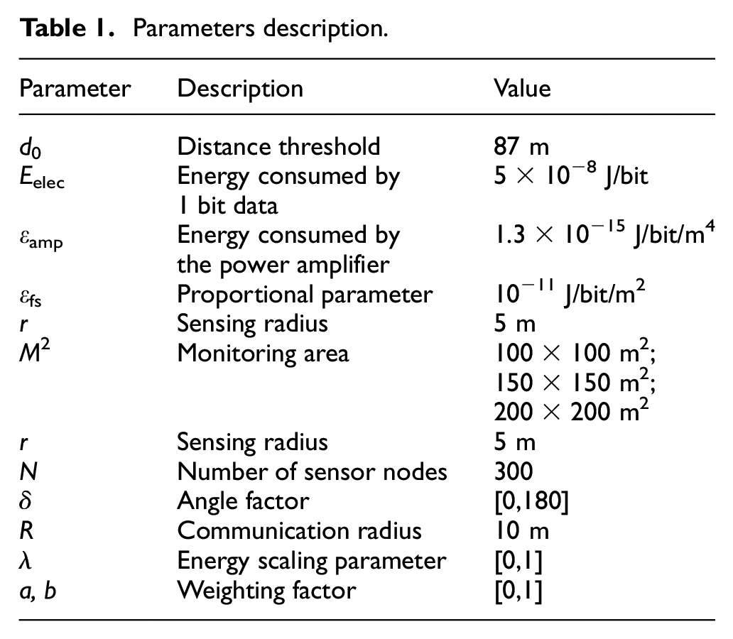
where the first energy consumption factor e_elec=5×10⁻⁸ J/bit, the second energy consumption factor ε_fs = 10⁻¹¹ J/bit/m², and the third energy consumption factor ε_amp=1.3 ×10⁻¹⁵ J/bit/m⁴. The parameter d₀ is the boundary between the free space model and the multipath model. In general, it is set as d₀=87 m.

Our work is to construct efficient routing, that is, to select an appropriate relay node for each node. The first goal our work is to minimize the total energy consumption of the network and improve the system longevity. Thus, this goal can be expressed as

minimize \sum_{i = 1}^{n} E_{i}

(3)

where E_i is the energy consumption of node i and n is the total number of nodes of the network.

The second goal our work is to balance the energy dissipation of all nodes of the network. Thus, the goal can be expressed as

minimize \sum_{i = 1}^{n} \frac{{(E_{i} - \bar{E})}^{2}}{n}

(4)

where $\bar{E}$ is the average energy dissipation of all nodes. This expression is to minimize the variance of energy dissipation of all nodes.

Proposed load-balancing routing

Our proposed load-balancing routing includes two steps: intrasegment routing and intersegment routing. The first step is to construct an initial routing for balancing energy consumption of each segment. The second step is to construct extra routing for balancing energy consumption between different segments.

Intrasegment routing

Intrasegment routing aims to construct routing within each segment, as shown in Figure 2.

Figure 2.

Intrasegment routing.

Based on this step, each node has a complete path to delivery data to the sink. The key idea of this step is to select appropriate relay node for each node. This step includes two phases: (a) building the basic transmission distance and (b) Constructing initial routing. According to the general transmission task distribution, nodes near the sink have more delivery tasks than those far away. Thus, nodes near the sink should adopt shorter transmission distances than those far away. Therefore, we design a basic transmission distance d_basic, as shown in Figure 3. This is a linear function of the distance to the sink, and is denoted as

D_{i} = {\begin{matrix} d_{0}, if d_{i} < d_{thresh} \\ d_{0} + A \frac{d_{i}}{d_{max}}, else \end{matrix}

(5)

where d₀ is the minimum transmission range of nodes, and it is used for nodes near the sink. In equation (5), d_i is the distance from node i to the sink; d_max is the maximum distance from any node to the sink; d_thresh is the distance thresh denoting the bound between near the sink and far from the sink; A is the slope of the increment of the basic transmission distance.

Figure 3.

Basic transmission distance.

Figure 3 shows that there are two periods regarding the basic transmission distance. In the first period, the value of the basic transmission distance is a constant. This period is used to guarantee enough relay nodes for relay selection. In other words, if the basic transmission distance is too small, there may be not relay nodes around the place with the basic transmission distance. In the second period, the value of the basic transmission distance increases when the distance from the node to the sink goes up. This period is used to balance the energy depletion of nodes in different places. The intrasegment routing includes two phases, which adopt different relay selection ways. In the first phase, all nodes have enough residual energy, and thus we do not consider the residual energy of nodes. In this phase, the relay selection is determined by the data delivery amount and the transmission distance. For any sensor node i, its relay node j is selected according to the following relay evaluation function

h (j) = a_{1} \frac{φ_{j}}{φ_{max}} + a_{2} \frac{| D_{i} - d_{ij} |}{d_{max}}

(6)

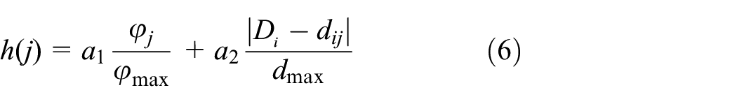
where ϕ_j is the amount of received data of node j, ϕ_max is the maximum traffic load of the network, D_i is the basic transmission distance of node i, d_ij is the distance between node i, and node j, d_max is the maximum distance between any two nodes of the network. Two parameters a₁ and a₂ are the weights of data traffic and transmission distance of equation (6).

The node j with the minimum value of equation (6) is selected as the relay node of node i. This equation indicates that we prefer to choose such a node as the final relay node: the node with less relay tasks and nearer the basic transmission distance. This design helps to balance the energy dissipation of the network. In the second phase, most nodes have little residual energy, so we need to consider the residual energy of nodes. In this phase, the relay selection is determined by the data delivery amount and the node’s residual energy. For any sensor node i, its relay node j is selected according to the following relay evaluation function

h (j) = b_{1} \frac{φ_{j}}{φ_{max}} + b_{2} \frac{E_{0} - E_{j}^{re}}{E_{0}}

(7)

where ϕ_j is the amount of received data of node j, ϕ_max is the maximum traffic load of the network, $E_{j}^{re}$ is the remaining energy of node j, E₀ is the initial energy of each node. Two parameters b₁ and b₂ are the weights of data traffic and residual energy of equation (7).

The node j with the minimum value of equation (7) is selected as the relay node of node i. This equation indicates that we prefer to choose such a node as the final relay node: the node with less relay tasks and larger residual energy. This design also contributes to balancing energy consumption of the network. There is a boundary between the above two phases of the intrasegment routing. This boundary is decided based on the remaining energy of the nodes near the sink. The first phase turns to the second phase when the average remaining energy of the nodes near the sink satisfies

\sum_{i = 1}^{N} \bar{E^{re}} < λ N E_{0}

(8)

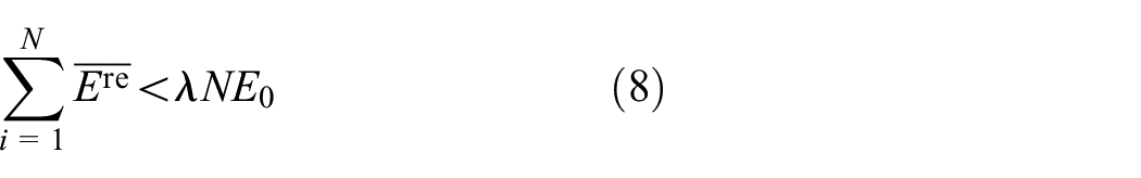
where $\bar{E^{re}}$ is the average residual energy of the nodes near the sink, E₀ is the initial energy of every node, and λ is the ratio of the average residual energy to the initial energy.

Intersegment routing

It is the intersegment routing, which aims to balance energy consumption among different segments. This is performed by the traffic load transfer mechanism, which aims to create a new path from one segment with more traffic load to another segment with less traffic load, as shown in Figure 4. Extra nodes are deployed along the new path. The path is determined by the genetic algorithm, which imitates the evolution actions of creatures and addresses a variety of optimization problems. This step includes the following phases:

Step 1: Our work focuses on partially- disconnected networks, each of which is partitioned into several isolated segments or near-isolated segments. We need to compute the traffic load of each segment near the sink. The traffic load Ω_k of segment k is calculated as

Ω_{k} = \frac{N_{k}}{N}

(9)

where N_k is the number of nodes of segment k, and N is the total number of nodes of the network. The traffic load transfer is performed from the segment with more transmission tasks to another segment with less transmission tasks.

Step 2: In genetic algorithm (GA), a chromosome is a solution and consists of several genes. In our work, each gene represents a sensor node, and the gene value means the node’s identity. Each chromosome C_i in the population is denoted as

C_{i} = (g_{i 1}, g_{i 2}, . . ., g_{iN})

(10)

where g_ij∈ {1,2,3,…, T+1} represents sensor node’s identity; j = 1,2,3,…, N; N is the total number of sensor nodes in the routing selection area; i = 1,2,3,… W; and W represents the number of organisms (i.e. chromosomes) in the initial population of the GA. Any chromosome of a segment starts from a node with large data traffic and ends at a node in the edge of the segment. Two chromosomes in adjacent segments can be combined into a new chromosome.

Step 3: The fitness function of the GA includes two forms. One is designed for the intrasegment genetic operation, and the other is designed for the intersegment genetic operation. In the intrasegment genetic operation, the fitness function is the length of the chromosome. In other words, we prefer to generate paths with short length. In the intersegment genetic operation, the fitness function is based on the hop (u, v) between two segments. The fitness function is designed as

f (u, v) = d_{uv} + δ_{uv}

(11)

where d_uv is the distance between node u of segment S₁ and node v of segment S₂, and δ_uv is the angle factor which is designed as

δ_{uv} = {\begin{matrix} C_{0} D_{u} < D_{v} \\ 0 D_{u} \geq D_{v} \end{matrix}

(12)

where D_u and D_v are the basic transmission distance of node u and node v, and C₀ is a constant which satisfies C₀ > 0.

Figure 4.

Intersegment routing.

In equation (11), the hop (u, v) with the minimum value of the fitness function is regarded as the final traffic load transfer path. In equation (12), the constraint C₀ > 0 means that there is a penalty if the path deviates from the sink. Thus, equations (11) and (12) indicate that we prefer to select the path with shorter distance and toward the sink. The genetic operation includes selection, crossover, and mutation.

In intrasegment genetic manipulation, the intersections are within segments, as shown in Figure 5(a) and (b). In the intersegment genetic operation, the intersection is the position between two segments, the first half of which can be regarded as Segment 1, and the second half as Segment 2, as shown in Figure 6(a) and (b). In this figure, there are four hops between Segment 1 and Segment 2, that is, (12, 33), (8, 48), (12, 48), and (8, 33). This hop connects two segments and determines the quality of the traffic load transfer. The crossover operation is to exchange a part of a chromosome between two chromosomes. For example, in this figure, Chromosome 1 and Chromosome 2 become Chromosome 3 and Chromosome 4 after the crossover operation.

Figure 5.

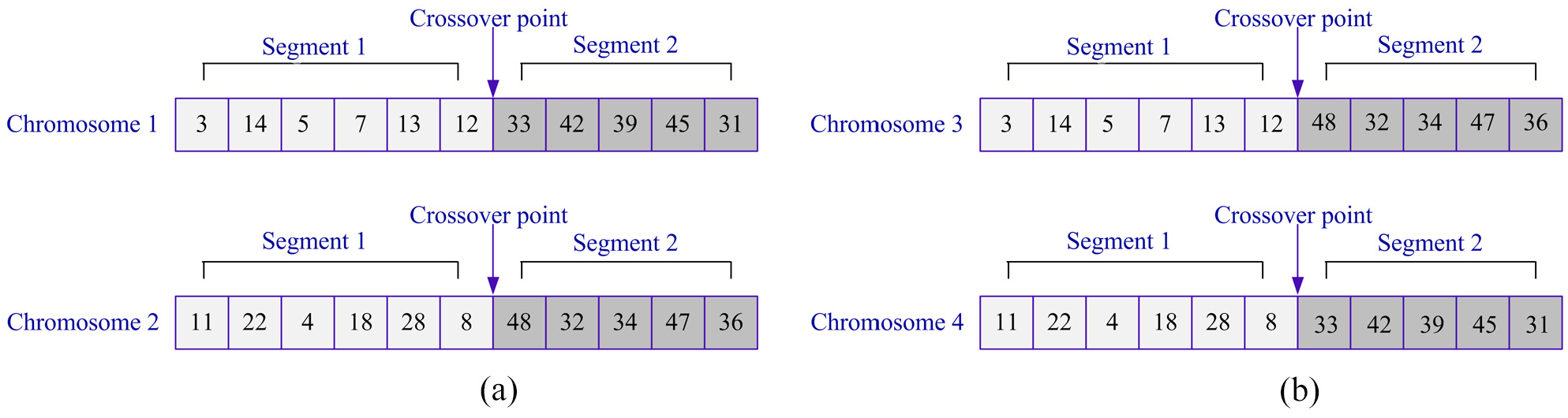
Chromosomes after the crossover operation (a) pro-chromosome data segment and (b) sub-chromosome data segment crossover operation.

Figure 6.

Chromosomes before the crossover operation (a) prochromosome data segment and (b) subchromosome data segment crossover operation.

Multisegment connection and GLBR algorithm

In multisegment, we consider the problem of planning the traveling path of a mobile sink in a disconnected network and reducing the overload of sensor nodes to maximize network lifetime. In every segment of the disconnected network, at least one Rendezvous Points (RPs) will be selected, therefore all sensor nodes can send their collected data to the mobile sink, then we consider the distribute of sensor nodes and add new RPs to reduce the sensor nodes’ energy consumption of relaying data, as shown in Figure 7.

Figure 7.

Multipoint routing using dual-BS (a) a RP located near the boundary, (b) two RPs located near the boundary and (c) multisegment routing.

The first RPs in every segment will be set up primarily as described in Section 4.2. There is one and only one RPs in each segment, after the subsequent steps, the selection of the RPs in some segments will be adjusted. The selection of RPs do not need to be adjusted in some segments which are more possible located near the boundary of the network, and these segments are call as “remote segments.” Specifically, whether a segment is a remote segment is determined by the stratification of the entire network, and all segments of the first layer are treated as remote segments. For these remote segments, selecting nodes near the boundary of segments can help reducing length of traveling path of mobile sinks, such as seg1, seg2, seg3, seg4 in Figure 7. On the other hand, the mobile sink needed to access three segments successively, and positions of RPs in the first segment and the third segment are known. The known two RPs can be used to determine the RPs of the second segment. Obviously, choosing the node which has minimum sum of distances to the known two RPs can reduce the length of mobile sink’s path maximally.

This article uses four segments to complete the routing process of discontinuous monitoring area. The process formed is to use the cluster head node in Segment 1 as the core routing forwarding node, and send a join request to the core routing for the new node to be added to the routing. After the core routing receives the request, it returns confirmation along the reverse routing, which constitutes a branch route. If the request information arrives at the cluster head nodes of other segments before reaching the core routing, the cluster head node sends the request information to the cluster head of Segment 1 to complete the establishment of branch routing. The total number of sensor nodes in the four segments is 300, and any segment has a cluster head node, and the sensing radius of the sensor node is 5 m. The routing process of the Intrasegment is as follows: when the sensor node has data to send, it first broadcasts a routing packet. The header of the packet includes all the destination address information. After receiving the packet, the next-hop router decides whether to receive and how to forward the packet according to the address of the packet header. The multicast routing data must be recalculated every time a node passes through. The relay node can cache the routing information that has been found, and within a period of time, the subsequent packet information will no longer contain all the destination address information, but will use the existing multicast routing table for forwarding.

Algorithm 1. GLBR algorithm.
Input: V = {V₁,V₂,…V_N}, set of sensor nodes in segments A = {A₁,A₂,…A_N }, set of representative node MAX_LAYER, the max layer of disconnected segments Set represent the visit order of nodes in GA(V) Output: RPs={RPs₁,RPs₂, …RPs_N}, set of RPs procedure PATH_ESTABLISHMENT begin find segments of the first layer, add corresponding A_i to RPs Current.Layer←2 whileCurrent.Layer<MAX_LAYER run GA algorithm to determine the visit order of nodes in RPs connect adjacent visits to form path lines check all segments whose layer are Current.Layer+1, add the node to RPs, the node should has the minimum sum of distances from itself to the two endpoints of the path lines in its segments Current.Layer++ end while end end procedure procedure PATH_OPTIMIZATION begin do Pre.Length← Calculate(RPs) I ← get the visit order of nodes in RPs fork=1 to Size (i)-2 do k++ form=1 to Size (Pre.Length) do optimize←true ture ++ m ++ end for end for whilek<=Pre.Length end end procedure

Algorithm 1. GLBR algorithm.

Input: V = {V₁,V₂,…V_N}, set of sensor nodes in segments
A = {A₁,A₂,…A_N }, set of representative node
MAX_LAYER, the max layer of disconnected segments
Set represent the visit order of nodes in GA(V)
Output: RPs={RPs₁,RPs₂, …RPs_N}, set of RPs
procedure PATH_ESTABLISHMENT
begin
find segments of the first layer, add corresponding A_i to RPs
Current.Layer←2
whileCurrent.Layer<MAX_LAYER
run GA algorithm to determine the visit order of nodes in RPs
connect adjacent visits to form path lines
check all segments whose layer are Current.Layer+1, add the node to RPs, the node should has the minimum sum of distances from itself to the two endpoints of the path lines in its segments
Current.Layer++
end while
end
end procedure
procedure PATH_OPTIMIZATION
begin
do
Pre.Length← Calculate(RPs)
I ← get the visit order of nodes in RPs
fork=1 to Size (i)-2 do
k++
form=1 to Size (Pre.Length) do
optimize←true
ture ++
m ++
end for
end for
whilek<=Pre.Length
end
end procedure

We consider the network consists of n segments and k sensor nodes. Our approach run O(k×n) times to find the center point by checking nodes in different segments one to one. In worst case, we use Graham scan to stratify the network, the network is divided into (n+1) layer, at this time each layer contains three segments and their representative nodes form a triangle. We check nodes in the next hierarchical segment to determine the RPs, therefore, the worst runtime complexity of path establishment is O(nk) × O(n), where O(n) is the time complexity to execute GLBR algorithm. The path optimization step has the same time complexity with path establishment. After the weighted selection of RPs, we determine the sink’s traveling path by the runtime complexity of O(n+1) × O(k). Thus, the worst overall time complexity of our approach is max (O((n+1)k) × O(n)) and O(k) × O(n+1). Usually in the actual application scenario, we have the condition of n, k or the value of n is constant, in these scenarios, the time complexity of our approach isO(k) × O(n+1). For a set of k elements, the typical time complexity of the GLBR algorithm is O(k×n).

Discussion

In this section, we evaluate the performance of our proposed strategy in terms of extra deployment cost, network lifetime, and load balancing degree. Our strategy is compared with other two routing schemes: IACO³⁷ and EEG.³⁸ In our simulations, the network size varies from 100 m × 100 m to 200 m × 200 m. The initial energy of each node is set as ε = 5.0 J. The ratio of the average residual energy to the initial energy is set as λ₁ = 0.2, λ₂ = 0.25, other parameters are set as: a₁∈ [0,1], a₂∈ [0,1], a₁+a₂ = 1; b₁∈ [0,1], b₂∈ [0,1]; b₁+b₂ = 1. The parameters of this article are shown in Table 1.

Table 1.

Parameters description.

Parameter	Description	Value
d ₀	Distance threshold	87 m
E _elec	Energy consumed by1 bit data	5 × 10⁻⁸ J/bit
ε _amp	Energy consumed by the power amplifier	1.3 × 10⁻¹⁵ J/bit/m⁴
ε _fs	Proportional parameter	10⁻¹¹ J/bit/m²
r	Sensing radius	5 m
M ²	Monitoring area	100 × 100 m²;150 × 150 m²;200 × 200 m²
r	Sensing radius	5 m
N	Number of sensor nodes	300
δ	Angle factor	[0,180]
R	Communication radius	10 m
λ	Energy scaling parameter	[0,1]
a, b	Weighting factor	[0,1]

To avoid errors caused by randomness, each simulation value is tested by 100 times, and the average value is regarded as the final result.

Figure 8 shows the extra deployment cost of the proposed GLBR in different network sizes and different network scales. For achieving traffic load transfer, we need to deploy extra nodes between two isolated segments. The extra deployment cost means the ratio of the number of the deployed extra nodes to the total number of nodes of the network. As shown in this figure, the overall trend of the ratio is that it decreases when the total number of nodes goes up. This is because the rise of the total number of nodes decreases the ratio. In the same network size, the variation in the number of nodes has little impact on the number of the extra deployed nodes. Furthermore, the rise of the network size increases the extra deployment cost by comparing Figure 8(a)–(c). This is because the rise of the network size increases the average distance between two isolated segments. Thus, more extra nodes are needed with the rise of the network size. In addition, the extra deployment cost varies from 3% to 6% in all times. This extra cost is acceptable and valuable. In other words, the network performance is improved at the cost of little overhead.

Figure 8.

Extra deployment cost under different parameters (a) λ₁ = 0.2, a₁ = 0.4, a₂ = 0.6, b₁ = 0.5, b₂ = 0.5; (b) λ₁ = 0.2, a₁ = 0.5, a₂ = 0.5, b₁ = 0.4, b₂ = 0.6; (c) λ₂ = 0.25, a₁ = 0.5, a₂ = 0.5, b₁ = 0.5, b₂ = 0.5. (a) 100 m × 100 m, (b) 150 m × 150 m and (c) 200 m × 200 m.

Figure 9 demonstrates the network lifetime of the three routing protocols. As shown in this figure, as a whole, the network lifespan declines when the total number of nodes goes up. The reason is that more nodes generate more data which need to be delivered by such nodes. Thus, the energy consumption of nodes will be increased. This figure also shows that a larger network size results in the decrease of the network lifetime by comparing Figure 9(a)–(c). This is because a larger network size leads to a larger transmission distance between two nodes. Thus, the energy consumption is increased with the network size. Moreover, GLBR has larger network lifetime than other two protocols all the time. This is mainly because of our traffic load transfer mechanism, which balances the energy consumption of different segments and accordingly extends the whole system longevity. In addition, IACO has larger network lifetime than EEG. This is because the iteration operation of IACO helps to find better paths compared with the relatively simple path selection in EEG.

Figure 9.

Comparison of three algorithms network lifetime (a) λ₁ = 0.2, a₁ = 0.4, a₂ = 0.6, b₁ = 0.5, b₂ = 0.5; (b) λ₁ = 0.2, a₁ = 0.5, a₂ = 0.5, b₁ = 0.4, b₂ = 0.6; (c) λ₂ = 0.25, a₁ = 0.5, a₂ = 0.5, b₁ = 0.5, b₂ = 0.5. (a) 100 m × 100 m, (b) 150 m × 150 m and (c) 200 m × 200 m.

Figure 10 shows the load balancing degree, which is represented by the energy dissipation of individual nodes near the sink. The selected nodes are distributed near the sink, because such nodes need more energy than that of other places. This figure also shows that a larger network size results in more drastic fluctuation by comparing Figure 10(a)–(c). This is because a larger network size leads to a larger transmission distance between two nodes. Thus, the energy consumption is increased with the network size. In addition, in this figure, different nodes have different energy consumption, but GLBR has more stable energy consumption than other two protocols. This is because the two load-balancing mechanisms in our GLBR. One is the unequal transmission distances, and the other is the traffic load transfer mechanism. Furthermore, IACO has more stable energy consumption than EEG, because the former has considered two aspects of load balancing: the residual energy of nodes and the minimum energy of nodes.

Figure 10.

Comparison of three algorithms energy consumption (a) λ₁ = 0.2, a₁ = 0.4, a₂ = 0.6, b₁ = 0.5, b₂ = 0.5; (b) λ₁ = 0.2, a₁ = 0.5, a₂ = 0.5, b₁ = 0.4, b₂ = 0.6; (c) λ₂ = 0.25, a₁ = 0.5, a₂ = 0.5, b₁ = 0.5, b₂ = 0.5. (a) 100 m × 100 m, (b) 150 m × 150 m and (c) 200 m × 200 m.

Conclusion

In this article, we propose a load-balanced routing scheme for extending the network lifetime in partially- disconnected WSNs. This routing scheme includes two types of routing building: intrasegment routing and intersegment routing. In the intrasegment routing, we adopt unequal transmission distances to build initial routing for intrasegment load balancing. In the Internet segment routing, we adopt the genetic algorithm to build extra routing between different segments for intersegment load balancing. The first unique character of our work is the network type. We investigate partitioned WSNs where there are several isolated segments. The second unique character of our work is the load-balancing way. We pursue load balancing from a global perspective rather than from a local one. Extensive simulation results demonstrate that, as compared with other two routing protocols, our proposed solution significantly improves network lifetime and load-balancing degree. Our future work is the routing design of WSNs in special environments with obstacles.

Future work mainly focuses on how to deploy heterogeneous nodes that communicate directly with sink nodes in dense areas to form super links, thereby changing the transmission path of network nodes and reducing the number of data forwarding to achieve the purpose of saving network energy and balancing node energy.

Footnotes

Handling Editor: Yanjiao Chen

Declaration of conflicting interests

The author(s) declared no potential conflicts of interest with respect to the research, authorship, and/or publication of this article.

Funding

The author(s) disclosed receipt of the following financial support for the research, authorship, and/or publication of this article: This work was supported in part by the National Natural Science Founding of China under Grants 61771015, 61931016, and 62101402; and National Natural Science Founding of Henan under Grant 202300410286; and Key Science and Technology Projects of Henan Province under Grant 212102210374; and Key Funding Project of Colleges and University of Henan Province under Grants 19A520006 and 20A520027; and Aviation Science Foundation of China (2020000108101), and China Postdoctoral Science Foundation (2021TQ0261, 2021M702547).

ORCID iD

Zeyu Sun

References

Sampathkumar

Mulerikkal

Sivaram

. Glowworm swarm optimization for effectual load balancing and routing strategies in wireless sensor networks. Wirel Netw 2020; 26: 4227–4238.

Zhang

Tang

Wang

, et al. Load-balancing rendezvous approach for mobility-enabled adaptive energy-efficient data collection in WSNs. KSII T Internet Inf 2020; 14: 1204–1227.

Keegan

Mtenzi

, et al. Energy-efficient load balancing ant based routing algorithm for wireless sensor networks. IEEE Access 2019; 7: 113182–113196.

Singh

Sharma

. HSCA: a novel harmony search based efficient clustering in heterogeneous WSNs. Telecommun Syst 2018; 67: 651–667.

Sun

Xing

Yan

, et al. CMTN-SP: a novel coverage-control algorithm for moving-target nodes based on sensing probability model in sensor networks. Sensors 2019; 19: 257.

Kong

Qiao

, et al. Adaptive relay chain routing with load balancing and high energy efficiency. IEEE Sens J 2016; 16: 5826–5836.

Liu

. Atypical hierarchical routing protocols for wireless sensor networks: a review. IEEE Sens J 2015; 15: 5372–5383.

Wang

Liu

Niu

, et al. Lightweight blockchain assisted secure routing of swarm UAS networking. Comput Commun 2021; 165: 131–140.

Peng

Liu

Wang

, et al. A user-defined location-sharing scheme with efficiency and privacy in mobile social networks. Sci Program 2020; 2020: 7832875.

10.

Zhang

Han

Cai

, et al. DOAMI: a distributed on-line algorithm to minimize interference for routing in wireless sensor networks. Theor Comput Sci 2019; 774: 1–13.

11.

Kavitha

Guravaiah

Velusamy

. CS-CGMP: clustering scheme using Canada Geese Migration Principle for routing in wireless sensor networks. Wireless Pers Commun 2020; 115: 1363–1384.

12.

Lai

Zhou

, et al. Energy efficient link-delay aware routing in wireless sensor networks. IEEE Sens J 2018; 18: 837–848.

13.

Liu

Shen

, et al. Characterizing data deliverability of greedy routing in wireless sensor networks. IEEE T Mobile Comput 2018; 17: 543–559.

14.

Peng

Liu

Wang

, et al. Multidimensional privacy preservation in location-based services. Future Gener Comp Sy 2019; 93: 312–326.

15.

Qin

Huang

Zhang

, et al. Energy efficient data correlation aware opportunistic routing protocol for wireless sensor networks. Peer Peer Netw Appl 2021; 14: 1963–1975.

16.

Yang

Postolache

. Sustainable multipath routing protocol for multi-sink wireless sensor networks in harsh environments. IEEE T Sustain Comput 2021; 6: 168–181.

17.

Yang

, et al. Cascading failures analysis of wireless sensor networks with varying routing schemes. IEEE Sens J 2021; 21: 10193–10203.

18.

Wang

Zhang

Yang

, et al. Genetic algorithm for energy-efficient clustering and routing in wireless sensor networks. J Syst Software 2018; 146: 196–214.

19.

Long

Ding

. Energy-aware routing in wireless sensor networks: a complex networks based approach. Int J Wireless Mobile Comput 2016; 11: 182–189.

20.

Rajaram

Kumaratharan

. Multi-hop optimized routing algorithm and load balanced fuzzy clustering in wireless sensor networks. J Amb Intel Hum Comp 2021; 12: 4281–4289.

21.

Liu

Dong

Ota

, et al. ActiveTrust: secure and trustable routing in wireless sensor networks. IEEE T Inf Foren Sec 2016; 11: 2013–2027.

22.

Zhang

Tao

Yan

, et al. Shortest-latency opportunistic routing in asynchronous wireless sensor networks with independent duty-cycling. IEEE T Mobile Comput 2020; 19: 711–723.

23.

Liang

Long

Mei

, et al. A distributed intelligent Hungarian algorithm for workload balance in sensor-cloud systems based on urban fog computing. IEEE Access 2019; 7: 77649–77658.

24.

Wang

Zeng

Lai

, et al. Data collection from WSNs to the cloud based on mobile fog elements. Future Gener Comp Sy 2020; 105: 864–872.

25.

Yang

Liang

, et al. Global and local reliability-based routing protocol for wireless sensor networks. IEEE Internet Things 2019; 6: 3620–3632.

26.

Teng

Liu

, et al. A novel code data dissemination scheme for Internet of Things through mobile vehicle of smart cities. Future Gener Comp Sy 2019; 94: 351–367.

27.

Liu

Qiu

, et al. Restoring connectivity of damaged sensor networks for long-term survival in hostile environments. IEEE Internet Things 2020; 7: 1205–1215.

28.

Hong

Zhang

Xiong

, et al. FADS: circular/spherical sector based forwarding area division and adaptive forwarding area selection routing protocol in WSNs. Ad Hoc Netw 2018; 70: 121–134.

29.

Wang

, et al. Sustainable and efficient data collection from WSNs to cloud. IEEE T Sustain Comput 2019; 4: 252–262.

30.

Sun

Zhang

Nie

, et al. CASMOC: a novel complex alliance strategy with multi-objective optimization of coverage in wireless sensor networks. Wirel Netw 2017; 23: 1201–1222.

31.

Sun

Yun

Song

, et al. CCAJS: a novel connect coverage algorithm based on joint sensing model for wireless sensor networks. KSII T Internet Inf 2016; 10: 5014–5034.

32.

Liu

, et al. RLC: a reinforcement learning-based charging algorithm for mobile devices. ACM T Sensor Network 2021; 17: 1–23.

33.

Liang

Obaidat

Liu

, et al. Resource scheduling based on priority ladders for multiple performance requirements in wireless body area networks. IEEE T Veh Technol 2021; 70: 7027–7036.

34.

Liu

Qiu

Wang

. Load-balanced data dissemination for wireless sensor networks: a nature-inspired approach. IEEE Internet Things 2019; 6: 9256–9265.

35.

Sun

Liu

, et al. CSR-IM: compressed sensing routing-control- method with intelligent migration-mechanism based on sensing cloud-computing. IEEE Access 2020; 8: 28437–28449.

36.

Peng

Wang

, et al. Generic and efficient connectivity determination for IoT applications. IEEE Internet Things 2020; 7: 5291–5301.

37.

Sun

Dong

Chen

. An improved routing algorithm based on ant colony optimization in wireless sensor networks. IEEE Commun Lett 2017; 21: 1317–1320.

38.

Hameed

Islam

Raza

, et al. Towards energy and performance-aware geographic routing for IoT-enabled sensor networks. Comput Electr Eng 2020; 85: 106643.

39.

Ren

Liang

, et al. Efficient algorithms for delay-aware NFV-enabled multicasting in mobile edge clouds with resource sharing. IEEE T Parall Distr 2020; 31: 2050–2066.

40.

Sun

Xing

, et al. A novel nodes deployment assignment scheme with data association attributed in wireless sensor networks. J Internet Technol 2019; 20: 509–520.

41.

Yang

Taleb

, et al. Spectrum sharing for secrecy performance enhancement in D2D-enabled UAV networks. IEEE Network 2020; 34: 156–163.

42.

Wang

Zhou

Chen

, et al. A three-layer privacy preserving cloud storage scheme based on computational intelligence in fog computing. IEEE T Emerg Topic Comput Intel 2018; 2: 3–12.

43.

Yang

. CARTA: coding-aware routing via tree-based address. Wirel Commun Mob Com 2020; 2020: 4730594.

44.

Liu

. Survivability-aware connectivity restoration for partitioned wireless sensor networks. IEEE Commun Lett 2017; 21: 2444–2447.

45.

Sun

Hou

, et al. MR-DFM: a multi-path routing algorithm based on data fusion mechanism in sensor networks. Comput Sci Inf Syst 2019; 16: 867–890.

46.

Liu

, et al. Low-cost collaborative mobile charging for large-scale wireless sensor networks. IEEE T Mobile Comput 2017; 16: 2213–2227.

47.

Liu

Wang

Jia

, et al. Quick convex hull-based rendezvous planning for delay-harsh mobile data gathering in disjoint sensor networks. IEEE T Syst Man Cy: S 2021; 51: 3844–3854.

GLBR: A novel global load balancing routing scheme based on intelligent computing in partially disconnected wireless sensor networks

Abstract

Keywords

Introduction

Related works

Mixed routing

Communication distance adjustment

Network model

Proposed load-balancing routing

Intrasegment routing

Intersegment routing

Multisegment connection and GLBR algorithm

Discussion

Conclusion

Footnotes

Declaration of conflicting interests

Funding

ORCID iD

References