
Abstract
Closed-form combat equations, such as the Lanchester and Helmbold relations, have long been used to describe battle outcomes at an aggregate level, but they do not directly provide probabilities of victory or expected combat duration. Building on this tradition, this paper introduces a probabilistic combat equation that predicts both quantities within a symmetric modeling framework for attackers and defenders. The model is evaluated using historical combat data and an empirical probability formulation, with results expressed as functions of the fractional exchange ratio. A systematic comparison of attacker and defender perspectives reveals a statistically significant asymmetry in how the two views diverge from empirical probabilities, even though the underlying model contains no built-in attacker advantage. This divergence varies nonlinearly with the fractional exchange ratio and remains robust across alternative linear and quadratic specifications, including a localized analysis near unity exchange. Importantly, the implied attacker advantage does not necessarily indicate intrinsic operational superiority. Rather, it may reflect asymmetries in the historical record, including unbalanced classification of battle outcomes, differing interpretations of attacker and defender victories, and a concentration of observations in exchange ratio regimes favorable to attackers. The results highlight both the strengths and limitations of probabilistic combat models when applied to historical data.
Keywords
1. Introduction
Combat equations have been studied for more than a hundred years. The Lanchester’s equations, formulated in 1914, are the most recognized and frequently applied deterministic combat equations. 1 These equations are solutions to differential equations that describe the attrition of two adversarial forces. Additional important closed-form combat equations include the Helmbold relation2–4 and the Willard equation. 5
These closed-form combat equations can predict the winner of a battle; however, they do not offer the probability of the attacker or defender winning the battle. Furthermore, these equations are not fully grounded in physical quantities or factors; their mathematical structure is phenomenologically derived. In this study, we address this gap in research by employing our probabilistic combat model, which describes the probability that the attacker (or defender) will win the battle and its expected duration.
By comparing these two equations derived from the same model for combat between two opposing sides, we can explore potential asymmetries in the outcomes for both the attacker and the defender. Our rationale is as follows: the underlying symmetry of the equations presumes equal parameters for each side. Should these equations fail to correspond to actual combat observations? It suggests that an asymmetry exists between the attacker and the defender, or that an additional element affects the combat success.
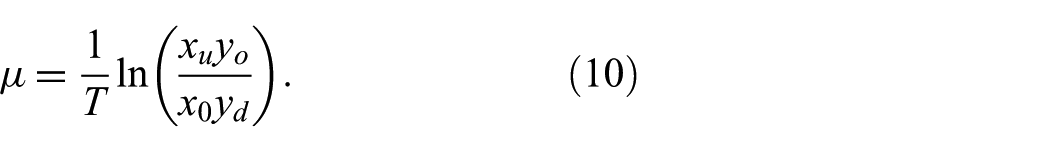
Our combat model examines individual battles, while this study seeks to determine whether there are general patterns that apply across all battles or specific parameter ranges.2,3 The results of our model, including probabilities and expected battle durations, are expressed as a function of the fractional exchange ratio, which has been identified as a suitable explanatory variable in previous research. 4 The fractional exchange ratio is defined as the ratio between the attacker’s casualty ratio and the defender’s casualty ratio.
Our main finding indicates that the model uncovers a slight, unexplained advantage for attackers across various fractional exchange ratios, irrespective of parameter values that correspond with observed probabilities and durations. This advantage is not noticeable in short- and low-intensity engagements. Several factors may contribute to this advantage, including the element of surprise, the motivation of the attacker, limited situational awareness of the defender, and potentially weaker defensive strategies. In addition, there could be a bias in recording the outcomes of battles that favors the attacker as the victor.
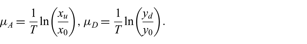
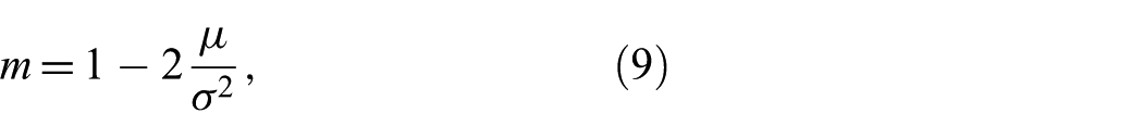
Furthermore, our comparison between the model’s results and empirical observations suggests that effective combat performance increases the probability of victory for the attacker or the defender more than our model dynamics predicts, when their casualty rates are more favorable than those of their opponent. This relationship can be illustrated using the fractional exchange ratio. We define the fractional exchange ratio, denoted as
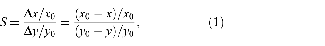
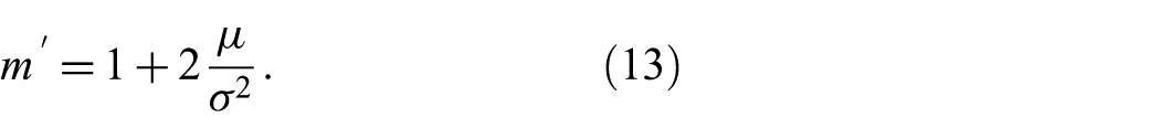
where
In this study, the attrition process is modeled using geometric Brownian motion. Although this choice supports analytical tractability, it also admits a clear operational interpretation. Classical deterministic combat models, such as Lanchester’s equations, describe attrition as proportional to force size and represent average combat dynamics under highly aggregated assumptions. The stochastic formulation adopted here extends this principle by retaining proportional mean attrition while incorporating uncertainty arising from variability in combat intensity, coordination, situational awareness, and effectiveness. Because uncertainty in losses scales with remaining force size, the model reflects empirically observed variability in combat outcomes and provides a quantitative basis for command-level decision-making under uncertainty, such as assessing the likelihood of success, expected duration of engagement, and the timing of continuation, reinforcement, or termination decisions. The formal specification of this stochastic combat model and its associated decision boundaries is presented in Section 4.
Within this stochastic framework, volatility and decision boundaries are introduced as model parameters because of the difficulties in deriving them directly from uncertain and limited empirical data. Volatility measures the degree of fluctuation observed in battle attrition data, while decision boundaries indicate the level of determination in deciding whether to continue or conclude a battle. In our model, both the attacker and the defender have decision boundaries to reflect their perspectives on their performance and the opponent’s position in combat.
Before introducing the formal model, we summarize the key assumptions underlying the proposed framework:
Combat attrition for both the attacker and the defender is represented as a stochastic process and modeled using geometric Brownian motion.
The relative drift of the attrition process is parameterized by the fractional exchange ratio, which serves as the primary explanatory variable.
Battle termination is governed by deterministic decision boundaries that represent commitment or stopping thresholds.
Decision boundaries are assumed to be linear functions of time for analytical tractability.
Volatility and decision boundary parameters are treated as model parameters due to the limited availability of time-resolved empirical data.
Empirical observations are analyzed using aggregated data over the observed duration of each battle.
2. Related work
Most macroscopic combat models operate on deterministic principles, with the Lanchester’s equations 1 being the most notable. 6 Although these equations have been widely analyzed and expanded, no specific formulation is particularly supported by historical battle data. 7
The study by Lucas and Turkes 8 examines how the Lanchester models align with detailed daily data from the battles of Kursk and Ardennes. The researchers found that none of the basic Lanchester laws—square, linear, or logarithmic—fit the data particularly well, nor did any significantly outperform the others. This suggests that the choice of law is not critical, as the right coefficients yield similar results. In addition, no Lanchester law with a constant attrition coefficient fits well. The study by Lucas and Turkes 8 concludes: ”The failure to find a good-fitting Lanchester model suggests that it may be beneficial to look for new ways to model highly aggregated attrition.”
At its core, Lanchester’s laws do not incorporate a termination mechanism unless one side’s forces are eliminated. In 1971, Robert L. Helmbold examined the validity of the break-point hypotheses as explanations of the outcomes of land combat battles by Helmbold. 9 In 1995, Jaiswal and Nagabhushana 10 introduced a rule implementing absolute or relative force sizes to set limits and derive expressions for the final forces’ sizes.
Combat models can be classified as static or dynamic, which refers to their independence or dependence on time. Early static models focused on the quantity of troops and weaponry, with outcomes predicted via weighted comparisons between opposing forces. By modifying force sizes, some of these elements can be integrated into closed-form combat models; for example, a single tank might be assigned a value equivalent to a certain number of soldiers. In 1985, T. N. Dupuy developed the Quantified Judgment Model (QJM), 11 which incorporates not only weapons and the size of forces but also human elements like leadership and morale, in addition to operational factors such as terrain and weather. This model determines a power potential value for each party and, if the power potential of side A surpasses that of side D, predicts that A will emerge as the winner.
The evaluation of the equivalent numbers of systems, weapons, and personnel presents a significant challenge. An approach for comparing various sources of military capability and determining the equivalent numbers of soldiers and system units is to optimize the total capabilities values. 12
Considerable efforts have been devoted to enhancing heterogeneous representation and attrition modeling. In particular, Bonder and Farrell 13 provided important information on attrition coefficients within heterogeneous settings. Nevertheless, their approach has drawbacks, such as inconsistencies in addressing parallel target acquisition. 14
In 1951, Morse and Kimball 15 pioneered a stochastic model for calculating time-dependent casualty probabilities for both attackers and defenders. Hausken and Moxnes16,17 explored stochastic war equations, while Kingman discussed stochastic variations of Lanchester models. 18 A comprehensive review of combat attrition modeling can be found in Fowler’s book. 6
The Helmbold relation is among the most recognized mathematical models for predicting combat outcomes. 2 The Helmbold relation is a mathematical expression that describes historical battle data. Helmbold first introduced the model in 1987, and the parameters in the formula were adjusted to empirical data from approximately 800 battles by Dean S. Hartley III in 2001. 3 Although it can be applied to both ancient and partially modern warfare scenarios, 4 there is still a lack of a theoretical framework or model to interpret the underlying structure of the equation.
Next, we introduce the Helmbold relation along with its associated variables. In this context,
where
Dean S. Hartley III carried out extensive research using empirical combat attrition data. 3 This work is based on the Helmbold relation, which incorporates various factors such as force sizes, environmental conditions, and human factors as explanatory variables to predict combat outcomes. The method relies predominantly on heuristics and does not incorporate models grounded in fundamental physical principles. This practical approach recognizes the difficulties in developing an all-encompassing theory considering many different factors.
Researchers in numerous studies have reported outcomes simulated using Lanchester models. Proposed enhancements include stochastic variations of Lanchester’s equations and probabilistic models employing Markov chains. Although these equations are widely applied, they present certain military and mathematical inconsistencies. Key issues include the convergence of stochastic models with their deterministic counterparts and the clear definition of mean combat outcomes.11,19
With increasing model complexity, finding analytical solutions may become impractical or computationally resource-intensive. Approximate solutions have been developed for resource-intensive problems, such as optimal resource allocation and asymmetric forces such as snipers and fighter jets. 20 Many of these models focus on estimating force sizes and attrition rates while typically overlooking the probabilities of victory or battle durations. Certain deterministic and stochastic models can be augmented with decision boundaries to assess these factors. This field of study provides opportunities for further exploration considering the differing objectives of detailed models and simple closed-form models. The former involves incorporating many explanatory variables, while the latter aims to provide a high-level understanding of the primary factors. A detailed literature review of stochastic and simulation approaches has been provided in Hartley. 3
3. Empirical data
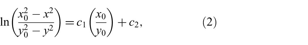
The research presented by Hartley 3 demonstrates that the Helmbold relation, as shown in Equation (2), is closely aligned with the observed data. The values were calculated using historical combat records, including information from the Land Warfare Database (LWDB) 21 which contains data from approximately 600 battles, as well as records from an additional 200 battles. 3 These records outline the initial and final sizes of the forces involved, the duration of the engagement, and indicate the winner, the attacker, or the defender.
Furthermore, another model known as the Oak Ridge Spreadsheet Combat Model (ORSBM) has been developed. 3 This model incorporates various variables, including force sizes, weaponry, human factors, operational variables, and environmental conditions. The primary focus of this model is to predict the force sizes at the end of the battles and to quantify the effectiveness of the battle.
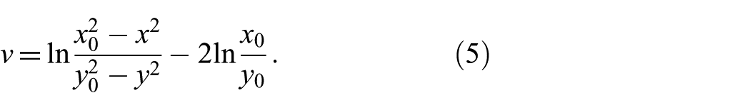
In addition, an empirical formula that estimates the probability of an attacker’s victory is provided by Hartley: 3
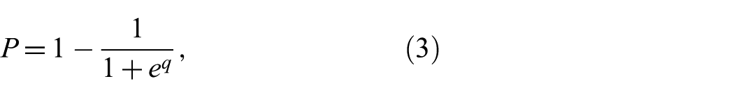
where

and
In Figure 1, the empirical data and points derived from the empirical formula show variations when plotted against the fractional exchange ratio, denoted as
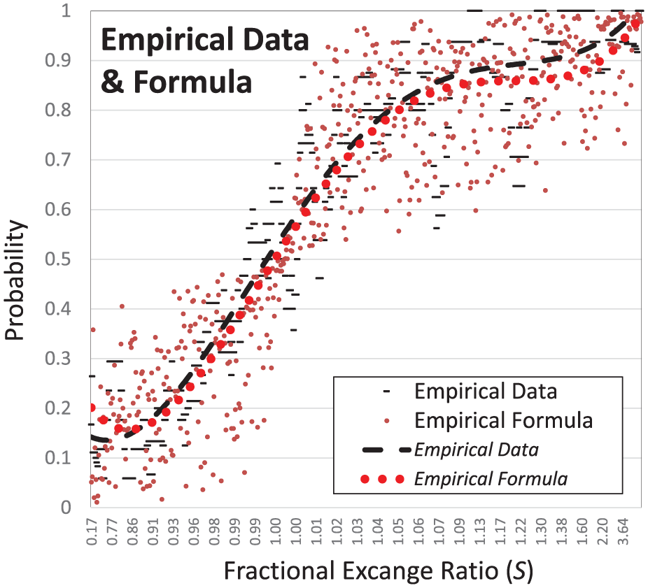
This figure illustrates the empirical probability (dashed) related to combat data, alongside a fourth-order polynomial approximation, both expressed as functions of the fractional exchange ratio (
The suitability and validity of using the logarithmic fractional exchange ratio
4. Model
Traditionally, closed-form combat models have been used to describe combat at a high operational level, helping us to understand and predict battle outcomes. These models typically incorporate the sizes of both the attacking and defending forces as key explanatory variables. Our model is designed to calculate the probability of victory for the attacker or the defender. We have developed a symmetric combat model that uses stochastic methods, presuming that force sizes adhere to a log-normal probability distribution. 22
The proposed model comprises two separate elements: one for stochastic processes and another that defines decision boundaries. In this study, the decision boundaries for opposing parties are formulated using win-lose decision thresholds. Situational conditions and decision criteria affect the complexity of these boundaries, which means that multiple factors influence them. We implement a basic linear model for the decision boundaries to demonstrate our approach.
The model parameters include the daily volatility of the attrition processes and the relative positions of the decision boundaries for both the attacker and the defender. These parameters can be interpreted in real-world contexts, and their appropriate values will be analyzed later in Section 5. In the model, a battle terminates when the losing force’s size dips beneath the lower decision boundary, suggesting surrender or operational decline. Concurrently, it is assumed that the force size of the victorious side meets the upper boundary limit. Although empirical data are unavailable, expert insight can provide information on decision parameter values. Another option is to construct a decision boundary model and infer model parameters from existing empirical attrition data. In this research, we choose the latter approach.
An important distinction between the Helmbold model and our model is that the Helmbold framework applies to the average reference line, dividing the empirical data into two groups. In contrast, our formula relates to individual data points. Furthermore, our method produces probability values, unlike the Helmbold relation, which does not yield probabilities, making direct comparisons unfeasible. Despite this difference, both models successfully predict the victor in battles in approximately 79% of the cases.3,12
The initial force sizes, attrition rates, volatility, and decision boundaries of the two opposing forces determine our combat equation. The combat model is divided into two parts. First, the attrition process is modeled as a stochastic process. Various alternatives include Brownian motion, geometric Brownian process, Poisson jump process, and more. We model the attrition process using geometric Brownian motion, in which stochastic changes are proportional to the process’ value. It is also necessary to formulate a model for decision boundaries. Decision boundaries can be modeled as either deterministic or stochastic functions. We use a linear deterministic function of time as a decision boundary model. The choice of a linear decision boundary is pragmatic and is dictated by constraints regarding both the quality and quantity of available empirical data, making exploring more general time-dependent or stochastic functions challenging.
The notion of decision boundaries is closely related to attrition processes and drift components. In our earlier research, 12 we introduced a model in which attrition processes were represented by the actual force sizes of both opposing sides separately. The slope of the attacker’s decision boundary was determined by the slope of the defender’s force size and vice versa. This model shows decreasing decision boundaries as opposing sides lose forces. 12
In Kuikka, 23 we take a slightly different approach. We define the stochastic process as the difference between the attrition processes of the attacker and the defender. This definition results in decision boundaries that remain constant over time. Although both approaches yield similar results regarding the probability of winning a battle, the former model does not allow for a standard way to model combat duration. In this study, we employ the second attrition process model and its decision boundaries, which allows us to apply existing mathematical results24,25 from the literature to determine the expected duration of combat using stochastic analysis techniques. 23
In real-world situations, the detailed temporal dynamics of attrition processes are typically unobserved, and most empirical data pertain only to initial and terminal force levels over a single engagement period. Consequently, variance must be treated as a parameter.
Let
Geometric Brownian motion is mathematically defined by the stochastic differential equation: 24

In this equation,
These characteristics can be assumed to describe an attrition process that, on average, corresponds to assumptions in the Lanchester equations. However, this correspondence is heuristic rather than a strict mathematical equivalence. Classical Lanchester models are deterministic force-interaction differential equations—most notably the cross-coupled square-law formulation—whereas geometric Brownian motion is a stochastic multiplicative diffusion process.
We examine a geometric Brownian process defined by the difference between the attrition processes of attackers and defenders. We use the drift definition
One advantage of modeling the difference between the two attrition processes is that it allows for the seamless inclusion of force reinforcements in the model. However, this aspect is particularly relevant when modeling individual battles. In our study, we base our assumptions on empirical data from Ref. 3, which we believe are consistent with the inclusion of force reinforcements and combatants represented in the figures, such as missing and wounded soldiers.
In the model application, decision boundaries are introduced as absorbing thresholds for the stochastic processes
For the attacker, the upper and lower absorbing boundaries are defined as

and for the defender as

The parameters
We denote the probability of the attacker’s victory as
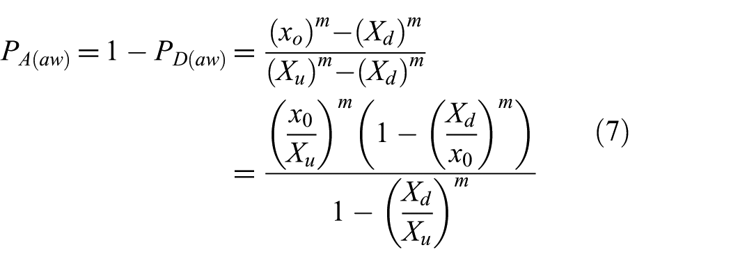
and
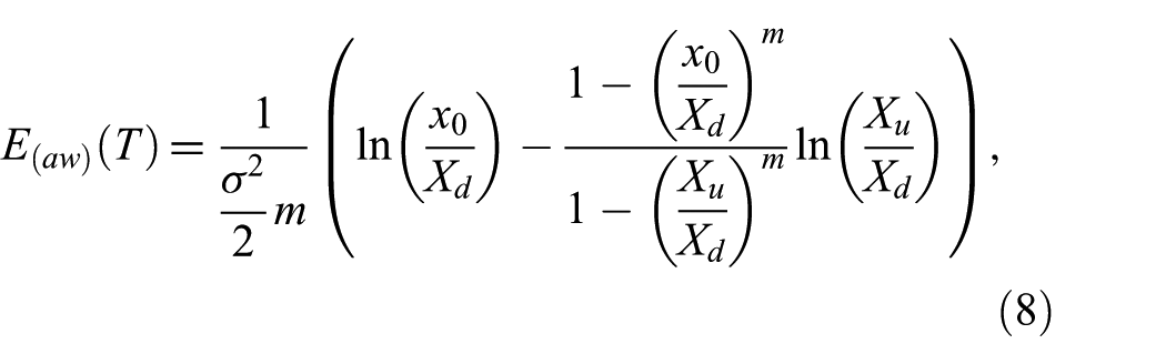
where
and
Similarly, for the defender view, the probability of the attacker winning the battle
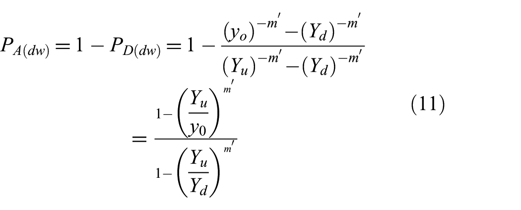
and
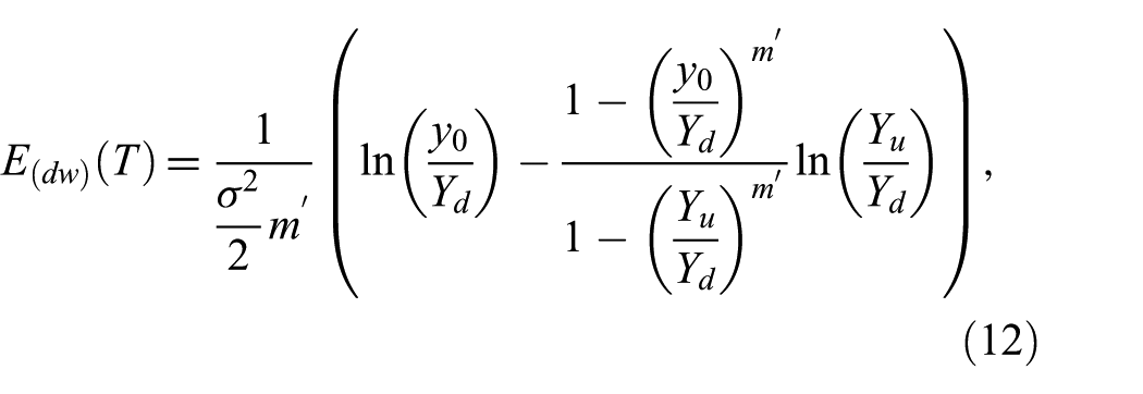
where
The parameters
5. Results
In Section 5, we examine the results of our combat model in several stages. In Section 5.1, we use the symmetric versions of Equations (7) and (8) to present the attacker view, while Equations (11) and (12) are applied for the defender’s view. In Section 5.2, we study how asymmetric decision boundaries influence the outcomes. Finally, in Section 5.3, we use symmetric phenomenological formulas to estimate the width of the decision boundaries and the associated volatility when the fractional exchange ratio is around
5.1. Results for symmetric decision boundaries
In this study, we use our combat model to calculate the probability of victory and the expected duration of the combats. Because data on combat volatility are limited, we incorporate it as a parameter within our model. Our objective is to determine a volatility value that aligns with two aspects of the model: the empirical probability of victory and the duration of combat. We investigate the differences between the observed probabilities of victory and those predicted by our model. Similarly, we compare the observed combat durations and expected durations predicted by our model. We aim to identify consistent volatility values and decision boundaries across both comparisons, indicating that the differences should be close to zero.
As shown in Figure 1, the empirical formula in Equation (3) and the empirical data yield comparable results. Therefore, we can employ either for our comparisons. In the following sections, we will use the empirical formula. To cover the possible range of volatility values, we calculate the probability differences and duration curves for six volatility values
An aspect to consider is contrasting the perspectives of the attacker and the defender to assess whether their outcomes vary and how these variations could influence potential advantages for each party. Ultimately, the attacker’s and the defender’s perspectives should produce similar results. This agreement is not guaranteed, as the formulas used in each case rely on either attacker-side or defender-side force size values.
A notable difference between the two could indicate a potential problem with the model that requires attention. It may also indicate that the attacker and defender are not positioned symmetrically in combats, demonstrating different decision boundaries and volatility values. In this study, we assume that our model approximately describes combats, and we focus on exploring any possible advantages for the attacker or defender during these encounters. Using individual decision boundaries and volatility values that are adjusted can lead to attacker and defender probabilities being similar. Our goal is to demonstrate that in our model the expected duration values can also align with the observed combat durations.
In our model, the decision boundaries define the stopping rules for combat scenarios. This is an important factor to consider when analyzing the advantages of attackers or defenders during combat. To examine these effects, we use some representative values for the decision boundaries and assume that they are equal for both winning and losing outcomes and for both the attacker and defender. This represents the symmetric situation, which we will discuss before exploring the asymmetric situation in Section 5.2.
To proceed systematically, we list the variations of the parameters in Table 1. We use the same parameters for the probability and duration calculations to find the matching values. First, we present the probabilities that an attacker will win a fight with the symmetric decision boundary parameter values of
This table details the parameters used to calculate the probability and expected duration of battles. The first column shows the corresponding figure numbers for the probability and expected duration calculations.
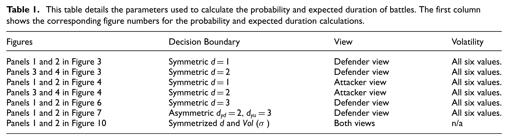
We aim to identify decision boundaries and volatility values that are reasonably consistent with the empirical results concerning probability and duration calculations. By discovering potential values for these variables, we may be able to draw conclusions about advantages for attackers or defenders that our current model does not directly take into account. These factors may result, for example, from the attacker’s surprise tactics or the defender’s protective capabilities.
To clarify our reasoning step by step, we present two cases in Figure 2: one with narrow decision boundaries and low volatility, and another with wide decision boundaries and high volatility. In the figures and subsequent captions, volatility is abbreviated as “Vol,” corresponding to the parameter
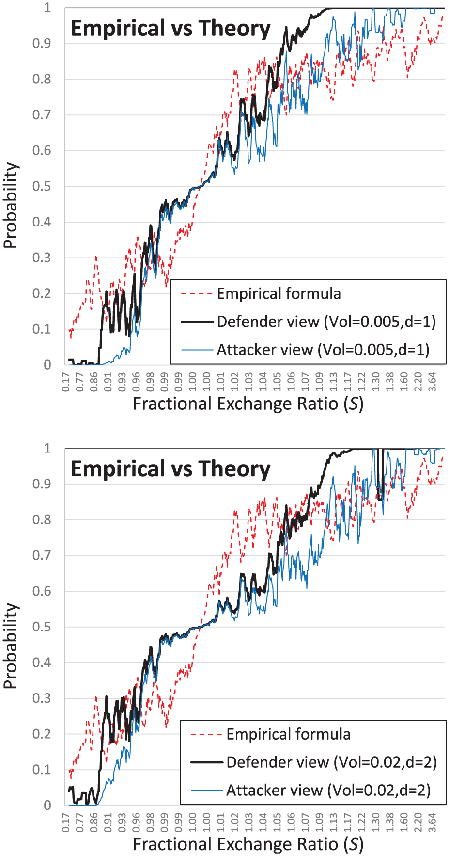
Empirical data curve (dotted) and two representative theoretical 7-period moving average curves (solid) illustrating the attacker’s probability of victory for both narrow (left) and wide (right) decision boundaries. “Vol” denotes the volatility parameter
Before exploring potential combinations of decision boundaries and volatility values, we examine the general observations of Figure 2. The curves on the left and right sides are largely mirror images of each other with respect to the fractional exchange value
In the middle range of
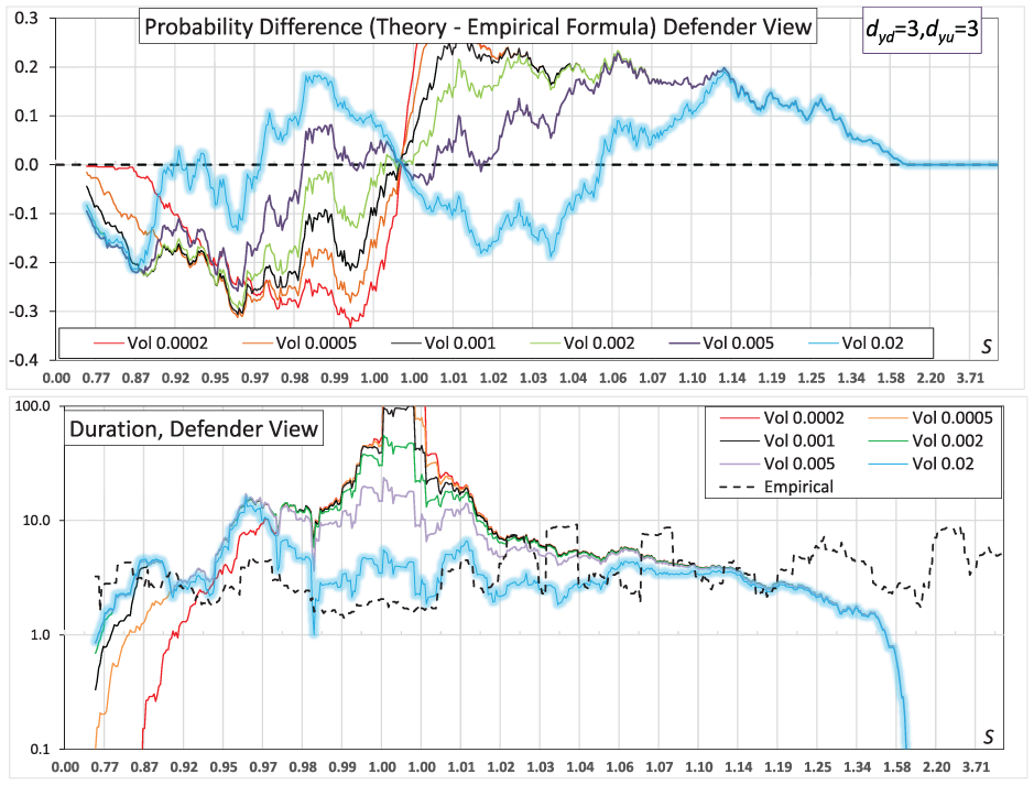
In Figure 3, the curves for the defender view reveal that when the decision boundary parameter value is set at
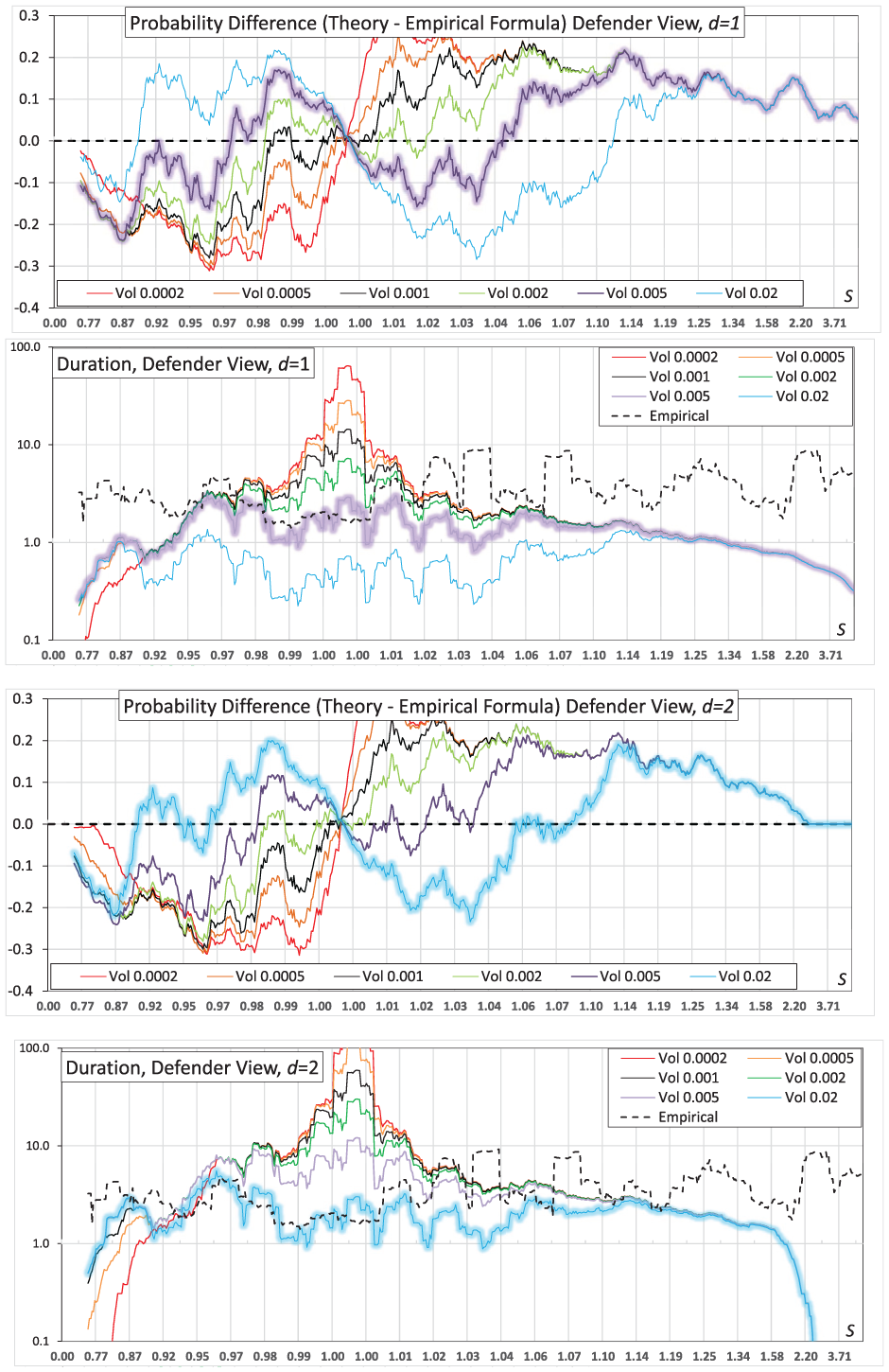
Defender view of the model: Comparing the probability and expected duration of attackers winning combats to empirical results (dashed lines). The model uses symmetric decision rules for
Higher parameter values
Figure 4 illustrates the attacker view of the attacker’s probability of winning and the expected duration of combats as a function of
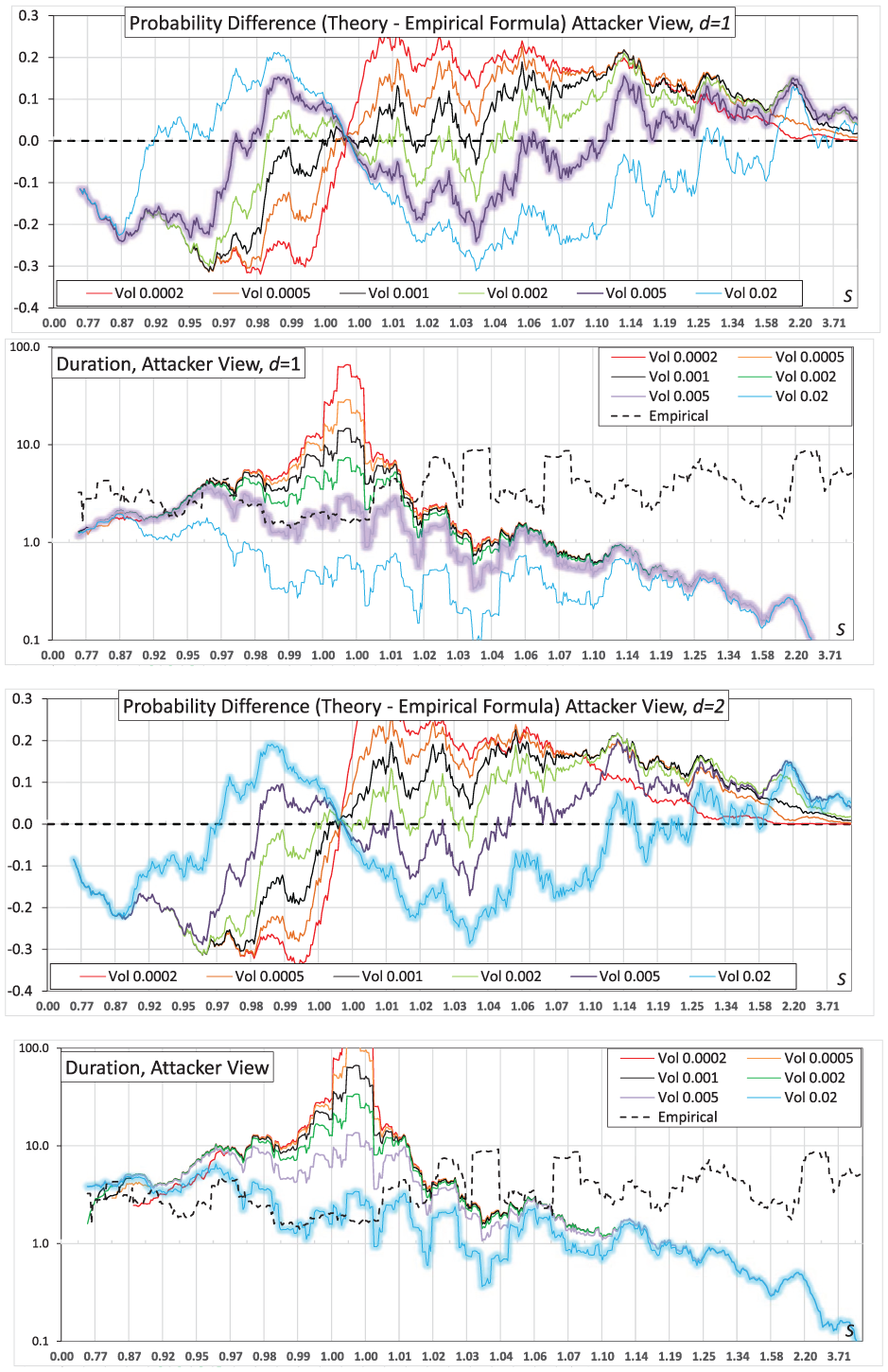
Attacker view of the model: Comparing the probability and expected duration of attackers winning combats to empirical results (dashed lines). The model uses symmetric decision rules for
Figure 5 illustrates the differences between the probability and duration curves of the defender and attacker view from Figures 3 and 4. The probability difference curve exhibits two peaks, one at low values and the other at high values of the fractional exchange ratio
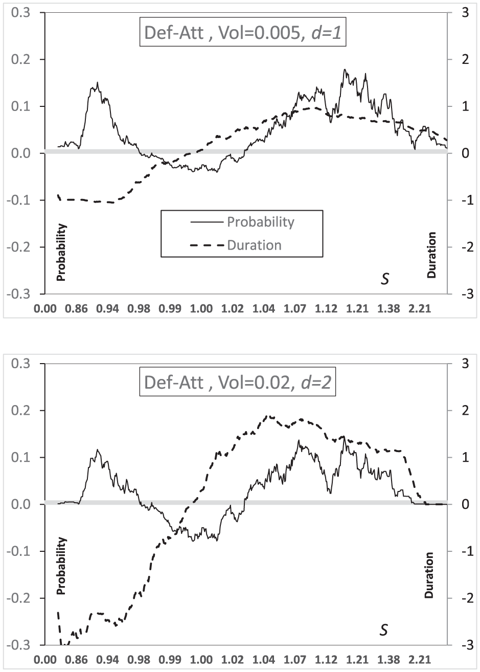
The results presented in Figure 5 indicate that attackers have an increased advantage at higher values of
The peak on the left side of the probability difference, which corresponds to low values of
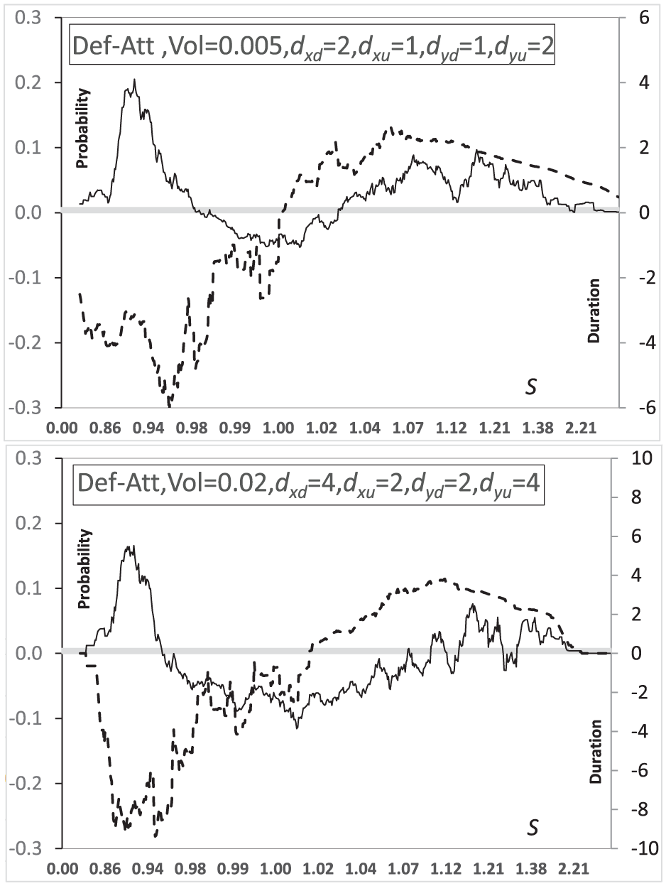
Finally, Figure 6 presents the defender’s perspective on the attacker’s probability of winning and expected combat duration for extra-wide decision boundaries
Defender view of the model: Comparing the probability and expected duration of attackers winning combats to empirical results (dashed lines). The model uses symmetric decision rules for
5.2. Results for asymmetric decision boundaries
The symmetric model in Section 5.1 is not fully aligned with the empirical probability results or the observed duration of the combats. Similar discrepancies can be detected in various parameter value domains, such as narrow decision boundaries combined with low volatility, or wide decision boundaries with high volatility. In this subsection, we explore the effect of asymmetric decision boundaries within the model.
The most significant discrepancy between the empirical results is observed in the middle range of the fractional exchange ratio for both scenarios: the first with the value of the decision boundary parameter of
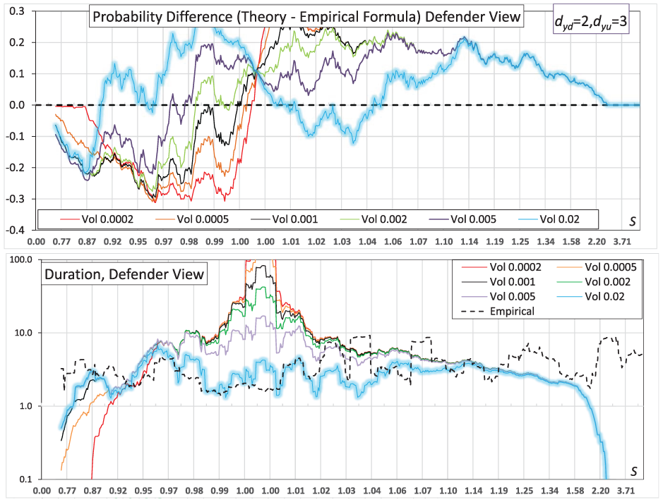
Defender view of the model: Comparing the probability and expected duration of attackers winning combats to empirical results (dashed lines). The model uses asymmetric decision rules for
In this example, the asymmetric decision boundaries tend to produce higher probability values for all values of
Figure 8 displays two different examples that illustrate the differences between the probability and duration curves of the defender and attacker view, which feature asymmetric decision boundaries. These show a pattern similar to that shown in Figure 5, which presents results with symmetric decision boundaries.
Two examples of the difference between the defender and attacker probability and duration curves with asymmetric decision boundaries.
From Figures 5 and 8, we can identify characteristic ranges for the fractional exchange ratio
5.3. Results for symmetric formulas of decision boundaries and volatility
To conclude our investigation, we use symmetric formulas for volatility and decision boundaries based on the fractional exchange ratio
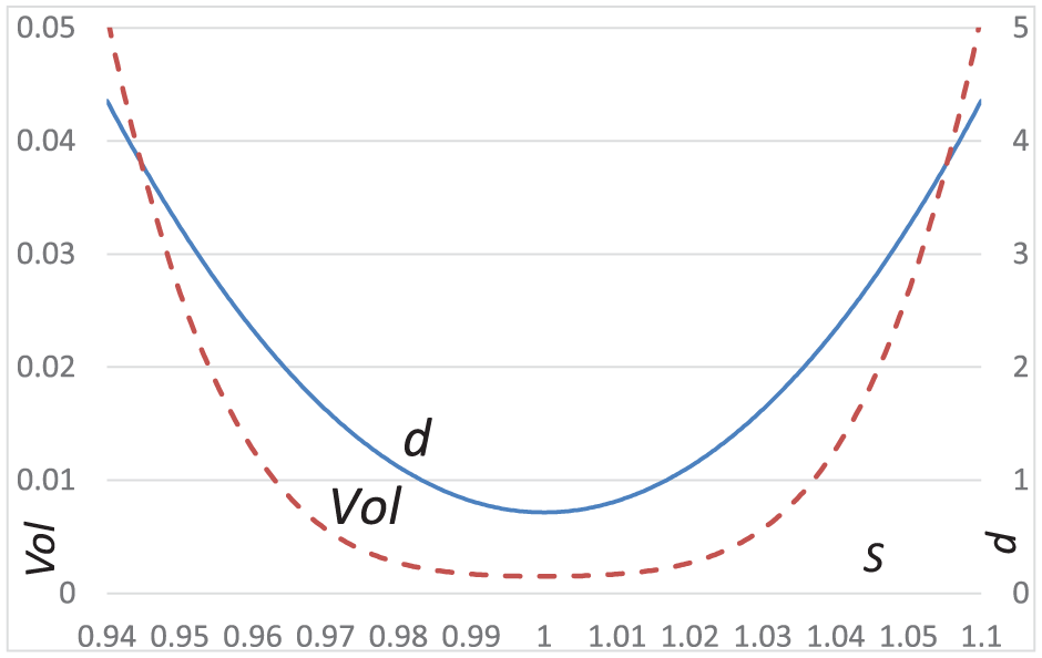
Symmetric curves for decision boundary parameters (
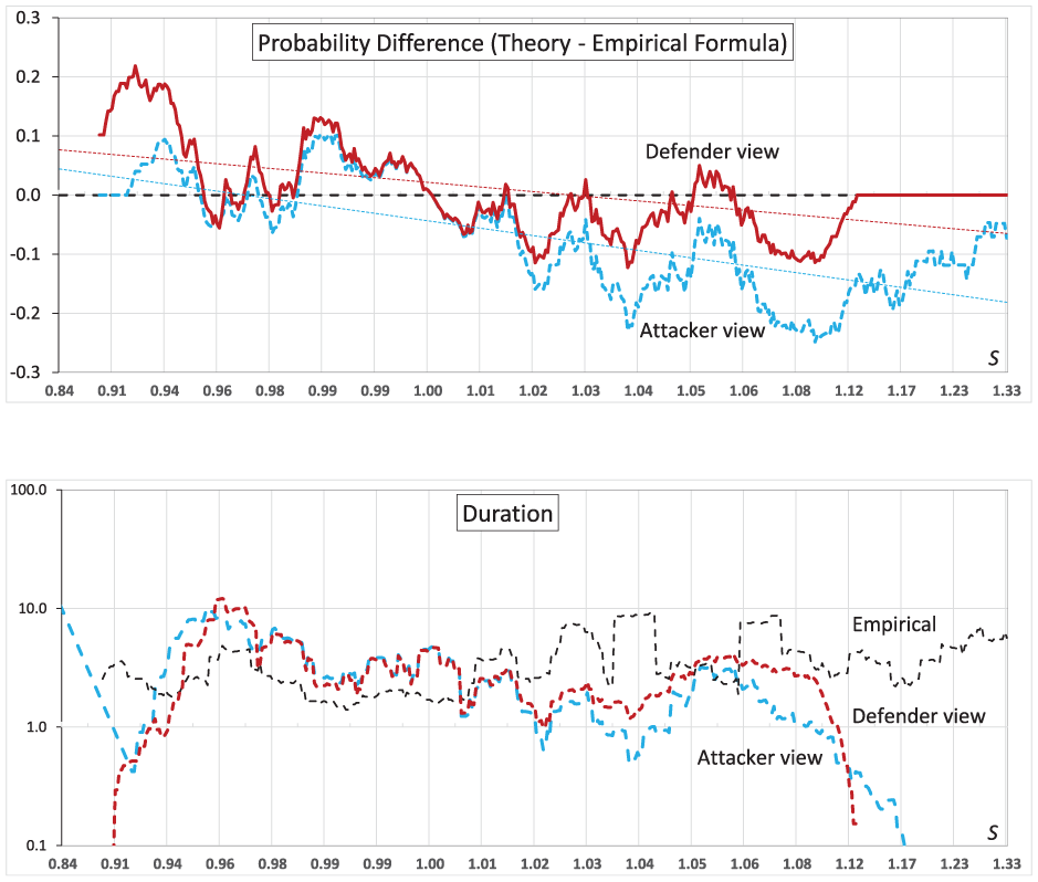
Top: Difference of theoretical probabilities and empirical observations for defender and attacker views with linear trend lines. Bottom: Theoretical expected durations for defender and attacker views compared with empirical observations. Theoretical results use symmetrical formulas from Figure 9.
Two key observations in Figure 10 can be drawn from the results on the symmetrized decision boundaries and volatility. First, both the defender and attacker views show a declining trend in the difference between theoretical predictions and actual observations as the fractional exchange ratio increases. Second, the attacker view exhibits a higher probability deviation from the expectations compared to the defender view at high values of the fractional exchange ratio
The decreasing trend in probability has an impact of approximately 10 percent across the entire range of the fractional exchange ratio, from
The second result indicates that the attacker’s perspective reveals a greater disparity from the empirical values than the defender’s perspective. This implies that the attacker’s view shows a more pronounced advantage for the attacker than the defender’s view. However, both perspectives yield similar results for fractional exchange ratios in the middle range, as illustrated in Figure 10. When the value of
Although the probabilities and durations for both the defender and the attacker should ideally yield equal values, the empirical data indicate that the attacker’s probability is considerably lower than expected. This suggests that it would be more effective to lower the attacker’s decision boundary, rather than to adjust the defender’s decision boundaries. Furthermore, as illustrated in Figure 10, the empirical duration exceeds the expected duration when
In summary, applying the symmetric volatility and decision boundary formulas depicted in Figure 9 that yield low values for these variables within the middle range of the fractional exchange ratio (around
6. Sign and trend analysis of attacker–defender differences
The purpose of this section is to distinguish between two related but conceptually different statistical questions arising from the comparison of attacker and defender perspectives. The first concerns the sign of the difference between the two views, that is, whether the attacker and defender perspectives exhibit a systematic offset in their probability differences relative to the empirical reference. The second concerns the trend of this difference as a function of the fractional exchange ratio. Conflating these questions may lead to incorrect interpretations of statistical significance, and they are therefore addressed separately. Specifically, although the defender-side probability differences are numerically higher, their predominantly negative sign implies that the attacker perspective exhibits a larger discrepancy relative to the empirical probabilities.
We define the difference between the defender and attacker perspectives as follows.

where
6.1. Sign of attacker–defender difference
Our primary research question concerns whether the attacker perspective shows a systematically larger discrepancy in magnitude from the empirical probability curve than the defender perspective. This question is addressed by examining the sign of

against the one-sided alternative
Throughout most of the observed range of the fractional exchange ratio,
To directly assess whether the attacker and defender perspectives produce systematically different assessments relative to the empirical reference, we examine the sign and magnitude of the difference
This result provides direct statistical evidence that, over most of the observed range of fractional exchange ratios, the attacker-based formulation deviates more strongly from the empirical probability curve than the defender-based formulation. The difference
The only notable exception occurs in a narrow region around the unity exchange ratio (
6.2. Trend and nonlinearity with exchange ratio
While the sign of
Across the full range of observed exchange ratios, a quadratic regression of

with the quadratic term highly significant (
To isolate local behavior near equilibrium, we additionally fit a quadratic model over the narrow interval

Within this interval, both linear and quadratic terms are strongly significant (linear:
Taken together, the sign analysis establishes that the defender curve lies above the attacker curve, while the trend analysis demonstrates that the magnitude of this divergence varies systematically and nonlinearly with the fractional exchange ratio. The distinction between these two results is essential: the p-values associated with the regression slopes and the curvature quantify the dependence on the exchange ratio, while the positivity of
It is important to note that the shaded regions in Figure 11 represent 95% confidence bands for the estimated mean relationship, not prediction intervals for individual observations. Given the relatively large number of data points and the dense coverage of fractional exchange ratios near unity, the fitted quadratic relationships are estimated with high precision, resulting in comparatively narrow confidence bands. These bands therefore quantify uncertainty in the average attacker–defender divergence, rather than the dispersion of individual battle outcomes.
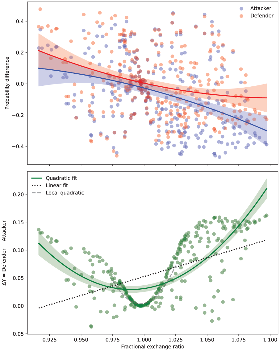
(Top) Attacker and defender probability differences versus fractional exchange ratio, with quadratic fits and 95% confidence bands for the fitted means. The upper band corresponds to the defender perspective, while the lower band corresponds to the attacker perspective. (Bottom) Difference between defender and attacker views (
7. Discussion
The results of this study indicate a systematic asymmetry between the attacker and defender perspectives when comparing model-based probabilities with empirical observations. Figure 11 summarizes this effect by showing the attacker and defender probability-difference curves (top) and their difference
A key question is whether the observed attacker advantage reflects a genuine operational superiority of attackers or instead arises from asymmetries in how combat outcomes are recorded and interpreted. Historical combat data are inherently noisy, incomplete, and subject to interpretation. In many engagements, the classification of a battle as a victory of the attacker or defender is not unambiguous and may depend on perspective, operational intent, or post hoc narrative framing. In particular, attackers may be more likely than defenders to interpret or report an engagement as a victory, especially in cases where objectives are partially achieved, forces disengage without annihilation, or outcomes remain contested. Such interpretative asymmetries can result in an imbalance in recorded outcomes that systematically favors attacker victories.
It is noteworthy that the attacker–defender divergence weakens in the immediate vicinity of unity exchange ratio. Engagements in this near-equilibrium regime are typically short and of lower intensity, which may limit the escalation of combat dynamics and reduce the emergence of pronounced asymmetries between attacker and defender assessments.
This potential bias is reinforced by the distribution of the empirical observations. The available datasets contain a larger number of data points with fractional exchange ratios greater than unity, corresponding to scenarios in which attackers inflict proportionally higher losses than they suffer. Because both empirical formulas and model-based probabilities increase with the fractional exchange ratio, an over-representation of observations in this regime naturally amplifies the apparent attacker advantage. As a result, even if attackers and defenders were operationally symmetric, asymmetries in outcome classification and data coverage could generate a statistical signal resembling a true attacker advantage.
From a modeling perspective, the symmetric structure of the proposed combat equation implies that, in the absence of such asymmetries, the attacker and defender views should coincide. The fact that they do not suggest either the presence of additional factors not captured by the model—such as surprise, morale, or initiative—or biases embedded in the empirical record itself. The analysis using symmetric and asymmetric decision boundaries shows that widening or shifting boundaries can partially reconcile model predictions with observed probabilities and durations, but these adjustments do not uniquely identify the underlying cause of the divergence.
Taken together, the findings indicate that the model reliably detects a statistically significant asymmetry between attacker and defender perspectives, while remaining agnostic as to whether this asymmetry reflects intrinsic combat dynamics or artifacts of data interpretation and reporting. Distinguishing between these explanations would require more granular empirical data, including clearer definitions of victory conditions and more balanced coverage across fractional exchange ratios. Future research aimed at disentangling operational effects from data-driven biases would therefore be valuable in refining both probabilistic combat models and their empirical validation.
8. Conclusion
This paper builds on an earlier probabilistic combat model developed by the author and applies it to extend the analysis beyond the phenomenological models of Hartley III and Helmbold. The approach explicitly incorporates volatility and decision boundaries, both of which have clear physical interpretations in the underlying system. Unlike previous phenomenological formulations, this framework links uncertainty to observable variability and decision structure, naturally producing battle duration, a feature absent from existing models. The observed attacker advantage arises not from the probabilistic method itself, but from the parametrized asymmetry embedded in the decision boundaries and volatility terms. Together, these features provide a physically grounded and operationally meaningful characterization of system behavior.
The research is based on a combat equation that uses the force sizes of the attacker and defender at the beginning and end of the combat. The model parameters, including volatility and decision boundaries, cannot be directly inferred from the empirical data due to the insufficient and uncertain nature of the empirical data. The probability of winning can be expressed from the perspective of the attacker or the defender, allowing an examination of potential advantages for both sides.
A key feature of the model is its symmetry with respect to the attacker and the defender. Using this symmetry, the effects of decision boundaries and volatility on combat outcomes were analyzed. By systematically varying these parameters, the study identified combinations that align with observed winning probabilities and battle durations, revealing discrepancies between the attacker’s and defender’s perspectives and indicating additional advantages not captured by the model variables alone.
The analysis focused on fractional exchange ratios as the primary explanatory variable. The attacker view exhibited greater discrepancies compared to empirical probabilities than the defender view, suggesting an additional attacker advantage beyond the modeled parameters. This trend was observed within and outside the middle range of fractional exchange ratios, indicating that the advantage may arise from factors such as increased self-confidence or endurance from previous combat performance. These findings were consistent in both the basic combat equation and the symmetrical analytical formulations, demonstrating the robustness of the model framework.
From an operational perspective, the model can be used to assess whether observed attrition dynamics and exchange ratios are sufficient to justify continued engagement, or whether termination thresholds are likely to be reached sooner than anticipated. By comparing attacker and defender perspectives, decision-makers can also identify situations in which confidence in success may be systematically over- or underestimated.
In conclusion, this study introduced a probabilistic combat model that explicitly incorporates uncertainty and decision boundaries, allowing the simultaneous analysis of victory probabilities and expected battle durations. By comparing attacker and defender perspectives within a symmetric modeling framework, the analysis revealed a statistically robust divergence between the two views when evaluated against empirical observations. While this asymmetry is consistently observed across most fractional exchange ratios, its interpretation remains open: it may reflect intrinsic features of combat dynamics not captured by the model, or alternatively systematic biases in historical outcome classification and data coverage. The results therefore highlight both the explanatory potential of probabilistic combat models and the importance of careful interpretation when confronting them with empirical battle data.
Footnotes
Funding
The author disclosed receipt of the following financial support for the research, authorship, and/or publication of this article: This work was supported by the Finnish Military Science Research Foundation sr. (Sotatieteiden tutkimussäätiö).
Declaration of conflicting interests
The author declared no potential conflicts of interest with respect to the research, authorship, and/or publication of this article.
Data availability
The empirical data used in this study have been adopted from the dataset provided by Hartley (2001) in the reference.