Sage Journals: Discover world-class research

Abstract

Quadratic fits are often used in regression and other modeling projects as either the whole of a model or part of a larger model. In this column, I discuss various small Stata devices that may help, including the twoway qfit command, calculation of the turning point position from coefficient estimates, and plotting the fitted curve over a wider range.

The main principles carry over from regression to various more complicated models such as generalized linear models. A specific example is the model known in statistical ecology as Gaussian logit, which is just a logit regression fitting a unimodal bell-like curve to a proportion as a quadratic function of some controlling variable.

The column includes commentary on wider historical, scientific, and statistical aspects of quadratic fits, with some remarks on their limitations and alternatives.

Keywords

st0794 quadratic fit linear fit turning points transformations Gaussian logit regression graphics twoway qfit twoway function stored results

1 Introduction: Example using auto data

Figure 1 shows some results from a simple analysis. The relationship between fuel efficiency (miles per gallon) as outcome or response and weight (in pounds) as predictor or explanatory or controlling variable was investigated for 74 cars in Stata’s auto data. Readers in many countries might appreciate some extra details. The observed range from 12 to 41 miles per gallon corresponds roughly to a range from 5.1 to 17.4 kilometers per liter. The observed range of weight from 1,760 to 4,840 pounds corresponds to a range from 798 to 2,195 kilograms.

Figure 1.

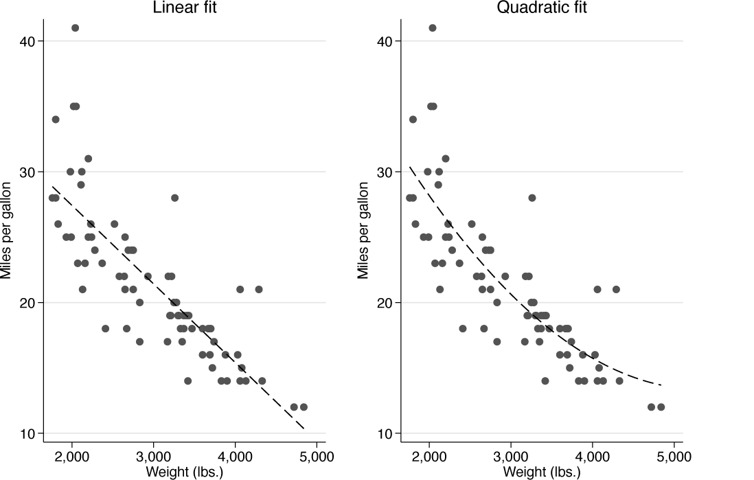
Linear fit (left) and quadratic fit (right) for fuel efficiency (miles per gallon) predicted from weight (pounds) for cars in the auto data

A linear fit seems quite helpful, but it does miss some evident curvature in the relationship. A researcher might also be perturbed by the implication that fuel efficiency would hit zero for a weight not enormously larger than the maximum in the data. Either way, we should consider whether a convex-down curve is a better idea than a straight line. A quadratic fit was tried next as an alternative. It does seem more convincing.

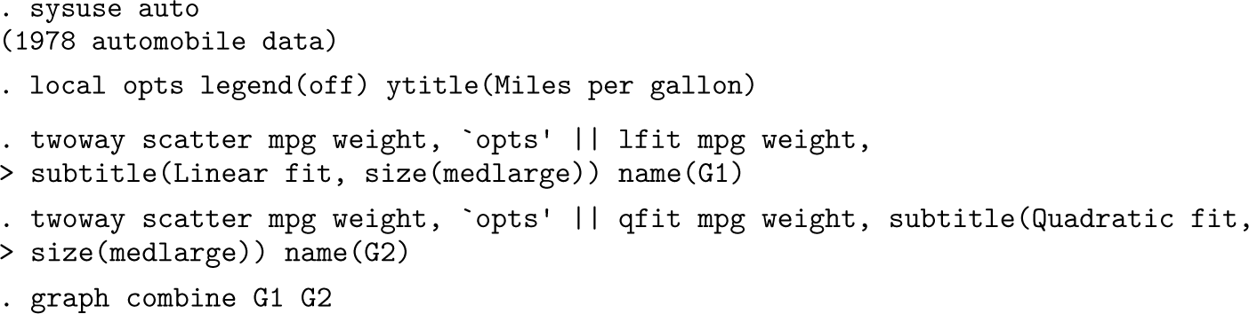
Here is the code behind figure 1. As usual, the code includes extra options added in hindsight to improve display.

This column gathers together some simple notes on the theme of quadratic fits in Stata: how to use them, when they might be useful, what they imply, what limitations they may have, and what alternatives might be considered.

Even a basic understanding hinges on knowing some mathematics: some geometry, some algebra, and some calculus. Roughly speaking, in the history of mathematics, geometry came first, with algebra and calculus following much later. See, for example, Heath (1921) or Netz (2022) on conic sections and Greek mathematics generally. See Kline (1972), Grattan-Guinness (1997), or Stillwell (2010) for a wider historical context.

If you are new to or rusty on the mathematics itself, many books in several styles give more detail. Older or more popular books may be as helpful as more recent or more formal texts: Compare, say, Hogben (1936 or any later edition), Abbott (1940, 1942), Hamming (1985), Spivak (1994), Gullberg (1997), or Strang (2017).

Similarly, the treatment here may be compared with accounts in just about any good statistical text, such as Sheather (2009); Ramsey and Schafer (2013); Whitlock and Schluter (2020); Wooldridge (2020); Maindonald, Braun, and Andrews (2024); or Faraway (2025). My impression is that although many researchers would regard the points that follow as standard, they are not often developed quite so fully in the literature.

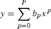
The first specific Stata lesson has already been given, which is that twoway includes twoway lfit and twoway qfit among standard subcommands. Sometimes, applying either or both subcommands indicates quickly that you can carry on with your initial idea or else that you need to do something different. Note also the twin commands twoway lfitci and twoway qfitci, which plot confidence intervals too.

2 Quadratics

For our purposes, we can focus on using a quadratic in a predictor variable x within a model predicting an outcome y. To keep notation as simple as possible, we let the context convey whether the discussion is about the functional form as part of a model specification or about a particular fitted curve to be compared with data. In general, such a quadratic has the form

y = b o + b_{1} x + b_{2} x^{2}

and its first and second derivatives (gradient or rate of change and rate of rate of change) are therefore

d y / d x = b_{1} + 2 b_{2} x and d^{2} y / d x^{2} = 2 b_{2}

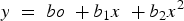
There are three coefficients defining a particular quadratic in this parameterization.

b_o, sometimes called an intercept or constant term, is what is predicted for y when x and so x² both are 0. It has the same units and dimensions as y.

b₁ as the coefficient of x has units and dimensions that are the units or dimensions of y divided by the units or dimensions of x.

b₂ as the coefficient of x² has units and dimensions that are the units or dimensions of y divided by the units or dimensions of x².

Working with units and dimensions may not always be needed, but for correct interpretation, it is vital to understand that the coefficients b₀, b_i, and b₂ do have quite different units and dimensions and so are not directly comparable.

Setting the first derivative, the gradient of the function, to 0 gives the position of the turning point of the quadratic, namely, $b_{i} + 2 b_{2} x = 0, o r x = - b_{1} / 2 b_{2} .$

A turning point is either a maximum or a minimum; what they have in common is that the gradient at any turning point is 0 so that the curve is momentarily flat. The two flavors of quadratic are exemplified in figure 2.

Figure 2.

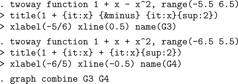
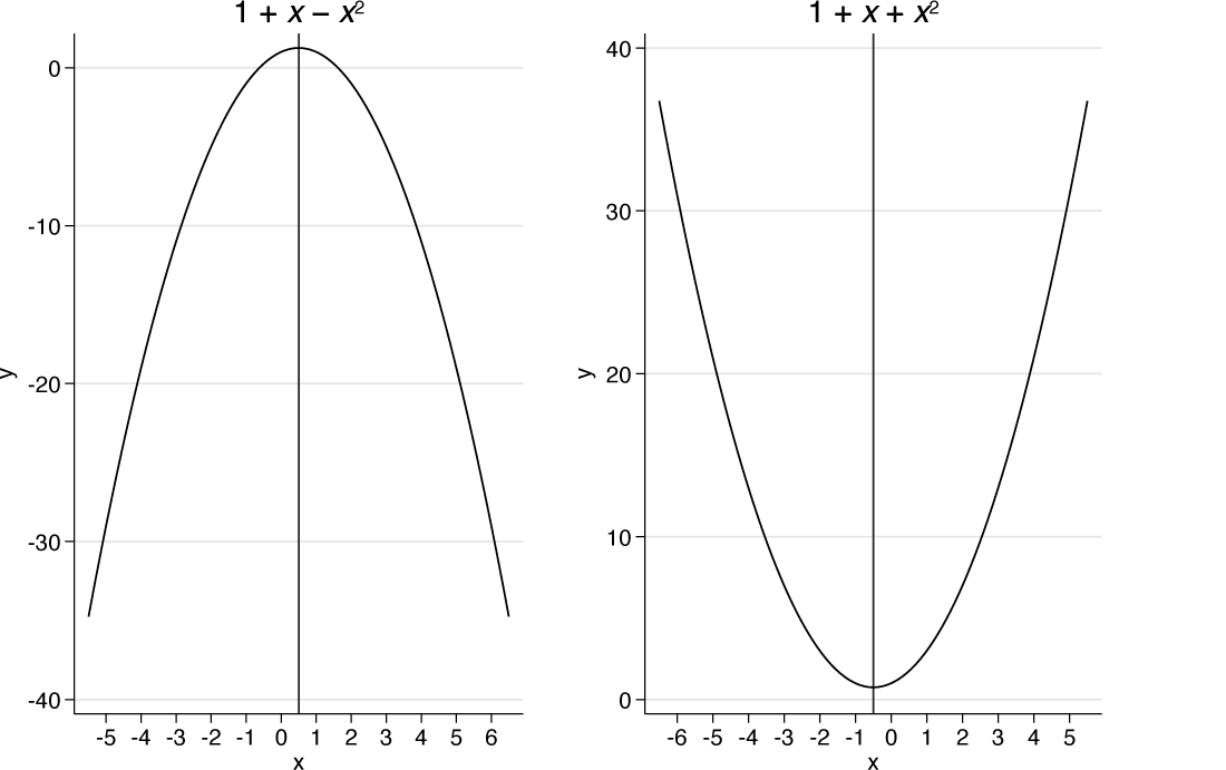
Examples of quadratics with turning points that are a maximum (left) and a minimum (right)

If you are new to the twoway function command, note that x is (exceptionally for Stata) just a placeholder for whatever is plotted on the horizontal or x axis. It is not the name of a variable that is, or should be, in the dataset. We just follow a common choice here in using the same symbol mathematically, but by doing so, we match the rule for twoway function. See the help or Cox (2004) for more detail.

See help smcl for the SMCL directives to produce superscripts and minus signs. The differences between hyphens, en and em dashes, and minus signs were the province of specialist typographers until we all gained access to software that would let us choose.

The quadratic $1 + x - x^{2}$ for which $b_{1} = 1, b_{2} = - 1$ is an example of the first flavor; its maximum is at $x = - 1 / - 2 = 1 / 2$ . Below that point, the curve is rising, so its gradient is positive, and above that point, the curve is falling, so its gradient is negative. The rate of change of the gradient given by $d^{2} y / d x^{2} = 2 b_{2} = - 2$ is consistently downward.

In contrast, $1 + x + x^{2}$ is an example of the second flavor; its minimum is at $x = - 1 / 2$ . Below that point, the gradient is negative and above that point, the gradient is positive. Its rate of change given by $d^{2} y / d x^{2} = 2 b_{2} = 2$ is consistently upward.

Quadratics like these are also sometimes called parabolas. In general, a parabola need not be symmetric about a vertical line, as is true in these examples.

Quadratics are examples of polynomials. We could consider the family

y = \sum_{p = 0}^{P} b_{p} x^{p}

where, for us, the maximum power P = 2.

In many models, a quadratic component is combined with other predictors. That adds complication without contradicting the discussion here. But, for example, if other predictors are present, the intercept or constant b₀ is what is predicted when all the other terms are zero. It is often still of interest and importance to focus on what the terms $b_{1} x + b_{2} x^{2}$ imply, given all other predictors. With a complicated model, however, the topography and even the topology of the fitted surface may make the idea of a single turning point less cogent. Still, whether a predictor is better handled with a single linear term or a quadratic may remain of concern.

3 Finding the turning point

As in the first section, we consider the variables mpg and weight from the auto data. We could fire up a quadratic fit directly with

However, we will just create a squared variable first, if only to avoid explanations using such factor-variable notation, which readers may not know.

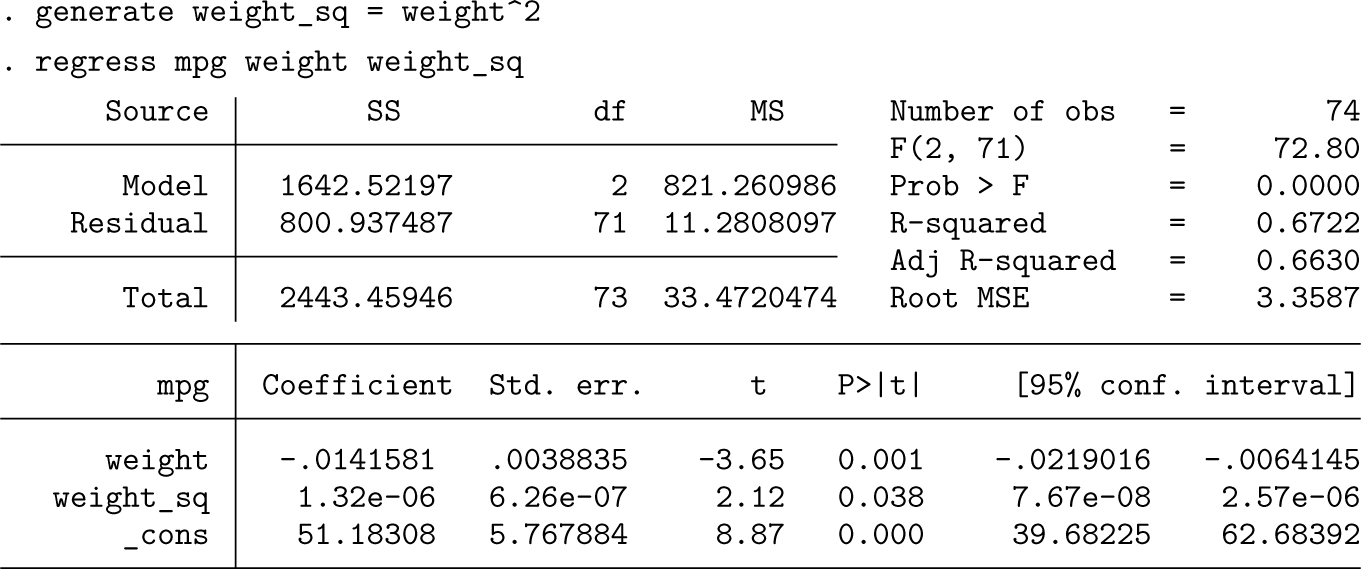
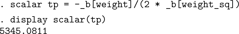
The quadratic fit does look quite good. We could read off the coefficients of weight and weight_sq interactively from the regress output and plug them into the expression for the turning point. However, that would not be an especially good idea. For a start, it is better to use an automated method, as might be used in a do-file or program, than to be dependent on interactive use. Furthermore, you would lose some precision that way, as Stata by default does not display to full precision in the regress output what it holds as coefficient estimates. Better practice is to calculate and store a result in (say) a scalar.

Let us focus on the Stata functionality being exploited here. After a model fit, the coefficient estimates are among the stored results and available in various forms.

A longstanding form that can be as useful as any other for our purposes is that the estimates are available in a special vector _b.

In this example, the coefficient of the variable weight is available in _b[weight], corresponding to b₁ in our notation. Similarly, the coefficient of its square, generated to be a variable weight_sq, is available in _b[weight_sq], corresponding to b₂. The intercept or constant is available in _b[_cons], corresponding to b₀. That is all useful, but watch out: such results are ephemeral and would be overwritten by the next similar command, whether another regress or a different model-fitting command. So you need to use coefficient estimates while they are available and save what you need to save.

We can save those estimates in various ways. Putting them in new variables is usually not to be recommended, unless you have (say) a wish to store several estimates in one variable. Otherwise, that would be inefficient. A scalar carries more precision than a global or local macro and can even be stored with a dataset. See help scalar for more information.

While keeping maximum precision in calculation is vital, especially in view of the need for reproducible research, full precision is not often needed in reporting. Citing the position of the turning point in a report to about 3 or 4 significant figures (say, 5,345 pounds) may be more than enough for most purposes.

As in any set of regression results, care must be taken in interpreting coefficients that have differing units and dimensions. Thus, the very small coefficient on squared weight can be assessed correctly only by bearing in mind the magnitudes that it multiplies. Concretely, for example, the co-medians of the weight data (the two middlemost ordered values in a set with even parity: Stigler [1977]) are 3,180 and 3,200 pounds, so the co-medians of the weight squared data are 10,112,400 and 10,240,000 squared pounds, respectively. As usual, the dimensionless t statistics are a better guide to relative importance.

4 Plotting the quadratic beyond the data range

It can be salutary to plot the fitted quadratic over a much wider range than is observed in the data, both to check the position of the turning point and to see the data and quadratic in context. In this case, no car can possibly have weight less than zero. But we can imagine cars, or at least other vehicles, that are much greater in weight than the observed maximum. In this case, plotting all the way to 10,000 pounds should be more than enough to see what is going on.

The technique here is to feed an expression based on the coefficient estimates to twoway function. Figure 3 shows the result.

Figure 3.

Data for fuel efficiency (miles per gallon) and weight (pounds) and quadratic fit in a larger context that includes the turning point

The point of such a graph may be private (just to understand yourself what has been done), pedagogic (to think aloud with students or colleagues about the fit), or even polemic (to argue that a model fit is somewhere between unsatisfactory and absurd).

5 What does fitting a quadratic mean?

There are several linked questions over quadratic fits. They all follow from the nature of a quadratic as a curve with a turning point.

Is it expected that a turning point would be observed in data?

Is the fitted turning point within or outside the range of the data?

Is the point of the quadratic merely to provide needed curvature in a relationship, or are there theoretical or at least subject-matter arguments for using that functional form?

These questions always arise, but sometimes, the answers may be too obvious to deserve emphasis. In some applications, it is well understood that using a quadratic is to impart extra curvature. In such cases, the idea remains that the relationship is monotonic over the observed data, meaning either increasing always or decreasing always and without a turning point. The fact that a quadratic if extrapolated beyond the range of the data yields absurd results may not be a fatal flaw. After all, much the same could be said about many linear fits, as every introductory statistics text should explain, and as already hinted in section 1.

Even when a quadratic has some physical or other basis, it may be only a partial or caricature model. A projectile thrown into the air (say, a ball or a stone) and pulled downward by gravity may be expected to trace a quadratic or parabolic path until it hits the ground. But air resistance alone can be a serious complication, as everyone finds who uses a paper dart or airplane as the projectile.

In other applications, it may be germane to underline that a quadratic fit is problematic, especially if there is a constructive alternative.

6 Transformations and other alternatives

There are almost always alternatives to using a quadratic.

We should mention in most detail the scope for using a transformation of the predictor, rather than the predictor and its square. The relationship shown in figure 1 could be modeled using the logarithm of mpg (and possibly also the logarithm of weight). Such exponential or power function relationships would show curvature but remain monotonic (and not imply that the relationship ever predicts zero or negative values). Another plausible choice is to use the reciprocal. In practice, some prefactor may also then be used for convenience. So, for example, 100 / mpg is the reciprocal of mpg multiplied by 100, so gallons per 100 miles. From an engineering point of view, such a fuel expenditure variable is quite as natural as the original fuel efficiency version.

If you are curious, you may want to try out these possibilities with the auto data and see for yourself that they all work quite well.

More generally, powers and logarithms remain the leading choices for transformations here. Choice and limitations of transformations remain large and occasionally controversial topics. Some comments and references in Cox (2024) touch on various recurrent issues. A model needs ideally to balance at least agreement with data, simplicity, and accordance with theory and other experience (Anscombe 1981, 123). Here agreement with data means not just that the functional form is suitable but also that handling of error matches as far as possible ideal or observed conditions to do with variability around the functional form.

There are yet other alternatives: nonlinear regression, generalized linear models, spline fits, scatterplot smoothing, and so on. Each of these has been the subject of several books, and each could be the subject of entire tutorials with Stata flavor, like this column. Inverse polynomials as particular generalized linear models (Nelder 1966; McCullagh and Nelder 1989) seem especially underrated. That aside, the merits and limitations of these approaches have sometimes sparked vigorous debate. See, for example, the lively discussion between Nelder, Ruppert, Cressie, and Carroll (1991).

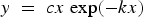
Here is a token example, however. The Ricker model prominent in fisheries research (Ricker 1954) features a linear term and an exponential term multiplied together:

y = c x \exp (- k x)

Here, in practice, c and k are both positive. It is another model with a turning point. As x tends to zero, so does y, and as x becomes arbitrarily large, y tends to zero. There is a turning point at x = 1/k, but the curve is asymmetric. For some references and applications, see Carroll and Ruppert (1988), Bolker (2008), or Ritz and Streibig (2008).

Riffing briefly: Simplicity as a goal or guide, even if elusive or illusive, is often recommended, or on the contrary, recommended against. Discussions range from the epigrammatic to entire monographs (for example, Sober [2015]). I like Alfred North Whitehead’s (1920, 163) summary, “Seek simplicity and distrust it”, as well as Sydney Brenner’s (1997; 2019, 67) warning against Occam’s Broom, “used to sweep under the carpet any unpalatable facts that did not support the hypothesis”. For the record, there is no evidence that Albert Einstein said that “A theory should be made as simple as possible, but not simpler”, or something to that effect (Calaprice 2011, 475). But someone else undoubtedly did.

7 Testing?

Some researchers feel obliged, whether they are following their own statistical logic or prevailing cultural convention, to test the coefficients of a quadratic fit against null hypotheses of zero value. As a matter of personal style, I do not usually let a significance test choose predictors for me. In this particular case, the two predictors x and x² are a double act. In scientific terms, whether a quadratic fit is to be preferred to a linear fit is a fair question that I tend to answer with a combination of graphical examination and subject-matter thinking.

Stata will let you test either coefficient separately, of x or of x². Indeed, regress prints a p-value for each. But such separate tests do not make much sense, if only because those predictors are highly correlated with each other in practice, often more than researchers think. See, for example, Jeffreys (1961, 232-233) and Good (1972).

Regardless of the strength of your intuition, you can calculate the correlation between a predictor and its square directly using correlate. In the auto data, the correlation between weight and its square is 0.9915. Does it surprise you that the result is so high? Were you thinking that the relationship is curved, not linear, so the correlation cannot be very high? If so, you are correct that the correlation cannot be exactly 1, unless exceptionally there are only two distinct data points, but there is no scatter about an exact deterministic relationship either. As always, the correlation measures how well a linear fit would work, and the answer is always quite well when data extend only over a moderate range.

8 Gaussian logit: Example with ecological data

A quite different example is a little more challenging statistically and scientifically except that it should be easy, given a little explanation, to see why the model to be used makes sense and works well.

In ecology, it is common to record the abundance of different kinds of organisms, such as different species (or of finer or coarser taxonomic categories [taxa], such as varieties or genera). As every gardener or naturalist knows well, for any taxon and any pertinent environmental control (temperature, moisture, shade, acidity, salinity, nutrients, whatever), conditions can be just right, even optimal, or not ideal one way or the other. So it can be too cold, about right, or too hot for a taxon to do well or even survive at all. This picture is a caricature but still a good starting point. If there are several different environmental controls, more predictors may be needed. Organisms are typically in competition for resources with others. Such extra details complicate the analysis without contradicting the main idea.

In some projects, relating present abundance to present controls is the main scientific concern. In others, the goal is to use present relationships to get quantitative predictions for past environmental controls.

Jongman, ter Braak, and van Tongeren (1995, 68) gave example data for the abundance of the radiolarian Spongotrochus glacialis as predicted from February sea surface temperature. They read off data from a graph given by Lozano and Hays (1976). A Stata dataset is included in the media for this column, which provides a sandbox for play.

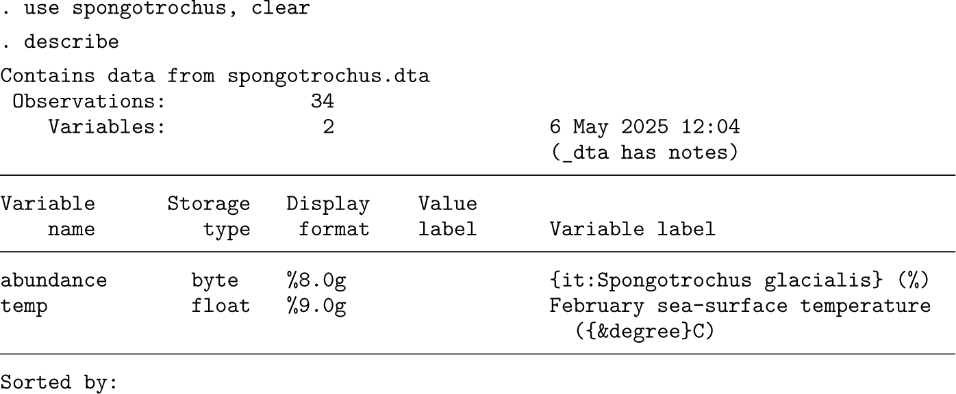
The SMCL elements in the variable labels look ugly in describe output but pay off in graphical results.

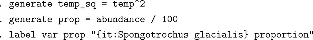
The data arrive as percent abundance, which, for our purposes, we scale to fractions or proportions between 0 and 1. You may want to glance ahead to figure 4, which shows the data as well as the model curve to be fit. The graph is suggestive of what statistically minded ecologists and ecologically minded statisticians call a unimodal response. As before, we create a variable containing squares.

For fractional responses, a model of some vintage now (Wedderburn 1974; Papke and Wooldridge 1996) adapts logit modeling for binary responses, coded 0 and 1, to the case of continuous proportions. For a concise and lucid account oriented to Stata use, see Baum (2008). For ecological applications, see Jongman, ter Braak, and van Tongeren (1995), as just cited, or the earlier work by ter Braak and Looman (1986).

The twist here is that using logit models with a predictor in quadratic form not only keeps predictions within the allowed range from 0 to 1 but also fits a bell-like shape to the relationship. As in logit models generally, predicted values remain positive but may become very small. The model has been dubbed Gaussian logit. The analogy with fitting a Gaussian (meaning, normal) curve is not exact, but the terminology seems helpfully evocative to me (and can easily be avoided if you disagree).

Mixing Stata syntax and mathematics, our model is that proportional abundance y and temperature x are linked by

y = invlogit (b o + b_{1} x + b_{2} x^{2})

where the inverse logit function invlogit() is exp()/{1 + exp()}. It is also often called expit() and indeed implemented under that name in some software.

The inverse logit function call for our case could thus be written out more fully as $\exp (b_{0} + b_{1} x + b_{2} x^{2}) / {1 + \exp (b_{o} + b_{1} x + b_{2} x^{2})}$

Where does the comparison with Gaussian curves come in? The probability density for a Gaussian or normal distribution is also proportional to an exponentiated quadratic with usual notation more like

\exp {(- 1 / 2) (x - u)^{2} / t^{2}}

Here u (think μ [mu] if you prefer) is the position of the peak (the mean, median, and mode of a Gaussian or normal distribution). u is equivalent to —b₁/2b₂, as already established. Further, t is a measure of the width of the bell. In ecological examples, that symbol can be taken to suggest tolerance, or how tolerant a taxon is to variations in an environmental control.

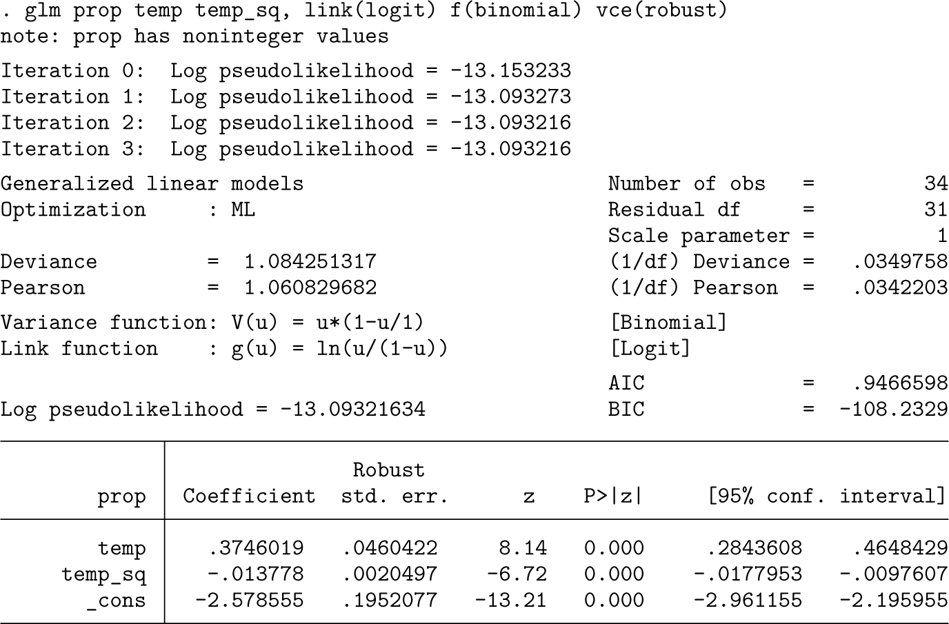
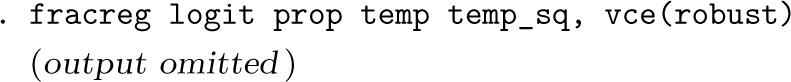
The model we use has long been available in Stata through application of the glm command. Specifying a binomial family is a justifiable fiction, and asking for robust standard errors is recognition of that. (As a hint, the variance of a proportion must approach 0 as the mean proportion approaches 0 or 1: the mean proportion can be 0 or 1 if all proportions are 0 or 1, and so variance is then, in either case, necessarily 0.)

To plot the predictions, we need to put them first in a new variable.

To get the position of the turning point, we can use exactly the same recipe as for plain regression. Pushing a quadratic through the inverse logit function stretches and squeezes its value y over different reaches of the support, but none of that has any effect on the position of the turning point in terms of x. The principle is simple and general: working with any monotonic transformation of the outcome leaves the turning point exactly where it was on the predictor scale. The only detail to notice, which should be clear anyway, is that there are transformations, such as the reciprocal, that change a minimum to a maximum, and vice versa.

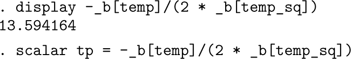
The turning point is about 13.6°C. We put the value into a scalar for future use. Now comes the plot at last (figure 4).

Figure 4.

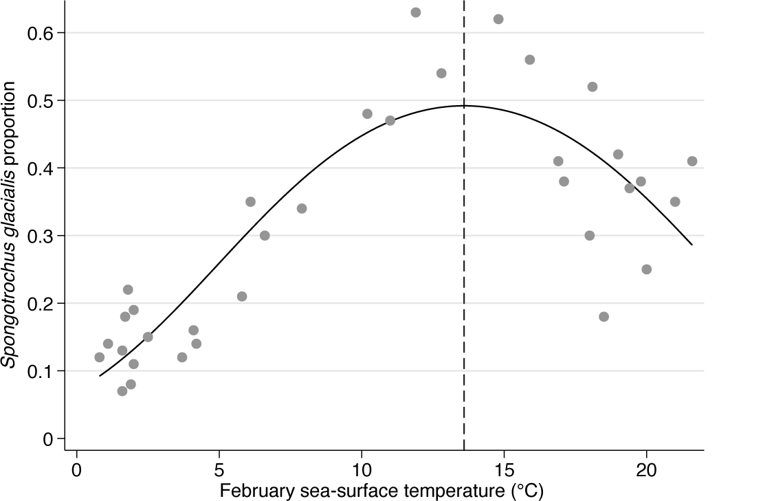
Data for Spongotrochus glacialis abundance and February sea-surface temperatures with a fitted Gaussian logit curve. The turning point with fitted peak abundance is at about 13.6°C. The curve has a symmetric bell shape.

Figure 5.

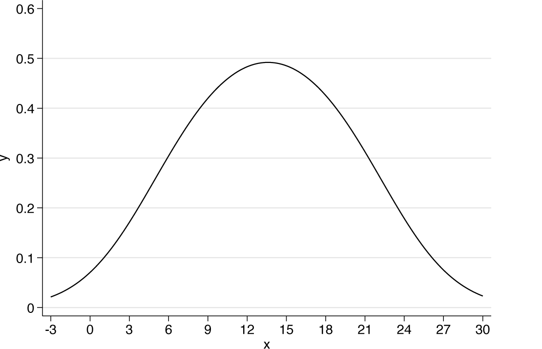
The fitted curve from the Gaussian logit model for Spongotrochus glacialis is here plotted over a wider range to show more of the bell shape

We claim success. The model seems to do a fair job of matching the data and ecological thinking.

Some details of the graph are personal choices, and as usual, your choices may differ. My own mix of wanting helpful detail and not wanting not-so-helpful detail leads to 00.1 0.2 0.3 0.4 0.5 0.6 as my preferred vertical axis labels. I do prefer showing 0 to 0.0, but I also prefer showing 0.5 to .5.

The bell shape is just about evident on figure 4, but to make it clearer, we plot over a wider range, stretching a little beyond what is physically plausible. See figure 5.

Stata 14 introduced an omnibus command, fracreg, for this purpose, so you may know it already or come to prefer it. Output from this command is essentially identical to that from glm, and so it is suppressed here to save space.

Regardless of which command you use, logit here remains one choice among several available. You may have preferences for other link functions, such as probit or complementary log-log. You may be tempted to experiment in any case. The term link functions is jargon especially familiar to users of generalized linear models (McCullagh and Nelder 1989), but it is not compulsory.

9 Conclusion

The small theme of quadratic fits in Stata raises many points, ranging from specific Stata techniques for obtaining and investigating such fits to matters of statistical and scientific taste and judgment in model specification, selection, and criticism.

The highlights of this column in Stata terms are as follows:

twoway lfit and twoway qfit are basic commands for initial exploration.

The coefficient estimates are available in _b[] after the model fit so that a simple calculation yields the position of the real or implied turning point. It is then a good idea to consider whether the existence of a fitted turning point is exactly what the analysis needs, an irrelevant distraction, or an implication that a different functional form should be considered given the data and the underlying science.

Similarly, the coefficients may be plugged into the equation for a quadratic and the corresponding curve plotted using twoway function. This graph is not too elementary to look at, even if it is too elementary to publish in your field. It can be useful privately, pedagogically, or even polemically. (Not the issue here, but plotting fitted polynomials with more terms can be even more salutary in dissuading oneself or others from overfitting.)

Finding the turning point of a quadratic can be done quite as easily if a quadratic fit is obtained working on some other scale using some monotonic transformation. In generalized linear model jargon, a link function other than identity itself makes no difference to the position of the turning point. The point arises often when using commands such as glm.

10 Programs and supplemental materials

To install a snapshot of the corresponding software files as they existed at the time of publication of this article, type

Supplemental Material

sj-dta-1-stj-10.1177_1536867X251398616 - Supplemental material for Speaking Stata: Some notes on quadratic fits

Supplemental material, sj-dta-1-stj-10.1177_1536867X251398616 for Speaking Stata: Some notes on quadratic fits by Nicholas J. Cox in The Stata Journal

Supplemental Material

sj-txt-1-stj-10.1177_1536867X251398616 - Supplemental material for Speaking Stata: Some notes on quadratic fits

Supplemental material, sj-txt-1-stj-10.1177_1536867X251398616 for Speaking Stata: Some notes on quadratic fits by Nicholas J. Cox in The Stata Journal

Footnotes

About the author

Nicholas Cox is a statistically minded geographer at Durham University. He contributes talks, postings, FAQs, and programs to the Stata user community. He has also coauthored 16 commands in official Stata. He was an author of several inserts in the Stata Technical Bulletin and is Editor-at-Large of the Stata Journal. His “Speaking Stata” articles on graphics from 2004 to 2013 have been collected as Speaking Stata Graphics (2014, College Station, TX: Stata Press). He is the Editor of Stata Tips, Volumes I and II (2024, also Stata Press).

References

Abbott

. 1940. Teach Yourself Calculus. London: English Universities Press.

Abbott

. 1942. Teach Yourself Algebra. London: English Universities Press.

Anscombe, F. J. 1981. Computing in Statistical Science through APL. New York: Springer. 10.1007/978-1-4613-9450-1.

Baum

C. F

. 2008. Stata tip 63: Modeling proportions. Stata Journal 8: 299–303. 10.1177/1536867X0800800212.

Bolker

B. M

. 2008. Ecological Models and Data in R. Princeton, NJ: Princeton University Press. 10.2307/j.ctvcm4g37.

Brenner

. 1997. Loose ends: In theory. Current Biology 7: R202. 10.1016/S0960-9822(97)70095-2.

Brenner

. 2019. Loose Ends … False Starts. Singapore: World Scientific. 10.1142/11496.

Calaprice

. 2011. The Ultimate Quotable Einstein. Princeton, NJ: Princeton University Press. 10.2307/j.ctvs32rgr.

Carroll

R. J.

Ruppert

. 1988. Transformation and Weighting in Regression. Vol. 30 of Monographs on Statistics and Applied Probability. New York: Chapman and Hall. 10.1201/9780203735268.

10.

Cox

N. J

. 2004. Stata tip 15: Function graphs on the fly. Stata Journal 4: 488–489. 10.1177/1536867X0400400413.

11.

Cox

N. J

. 2024. Speaking Stata: Quantile-quantile plots, generalized. Stata Journal 24: 514–534. 10.1177/1536867X241276114.

12.

Faraway

J. J

. 2025. Linear Models with R. 3rd ed. Boca Raton, FL: Chapman and Hall/CRC. 10.1201/9781003449973.

13.

Good

I. J

. 1972. Note: Correlation for power functions. Biometrics 28: 1127–1129. 10.2307/2528645.

14.

Grattan-Guinness

. 1997. The Fontana History of the Mathematical Sciences. London: Fontana Press.

15.

Gullberg

. 1997. Mathematics: From the Birth of Numbers. New York: W. W. Norton.

16.

Hamming, R. W. 1985. Methods of Mathematics Applied to Calculus, Probability, and Statistics. Englewood Cliffs, NJ: Prentice-Hall.

17.

Heath

T. L

. 1921. A History of Greek Mathematics. London: Oxford University Press.

18.

Hogben

. 1936. Mathematics for the Million. London: George Allen and Unwin.

19.

Jeffreys

. 1961. Theory of Probability. 3rd ed. London: Oxford University Press.

20.

Jongman

R. H. G.

ter Braak

C. J. F.

van Tongeren

O. F. R.

, eds. 1995. Data Analysis in Community and Landscape Ecology. Cambridge: Cambridge University Press. 10.1017/CB09780511525575.

21.

Kline

. 1972. Mathematical Thought from Ancient to Modern Times. New York: Oxford University Press.

22.

Lozano

J. A.

Hays

J. D.

. 1976. “Relationship of radiolarian assemblages to sediment types and physical oceanography in the Atlantic and Western Indian Ocean”. In Investigation of Late Quaternary Paleoceanography and Paleoclimatology. GSA Memoirs, edited by R. M. Cline and J. D. Hays, vol. 145: 303-336. Boulder, CO: Geological Society of America. 10.1130/MEM145-p303.

23.

Maindonald

J. H.

Braun

W. J.

Andrews

J. L.

. 2024. A Practical Guide to Data Analysis Using R: An Example-based Approach. Cambridge: Cambridge University Press. 10.1017/9781009282284.

24.

McCullagh

Nelder

J. A.

. 1989. Generalized Linear Models. Vol. 37 of Monographs on Statistics and Applied Probability, 2nd ed. London: Chapman and Hall/CRC. 10.1201/9780203753736.

25.

Nelder

J. A

. 1966. Inverse polynomials, a useful group of multi-factor response functions. Biometrics 22: 128–141. 10.2307/2528220.

26.

Nelder

J. A.

Ruppert

D. M.

Cressie

Carroll

R. J.

. 1991. Generalized linear models for enzyme-kinetic data. Biometrics 47: 1605–1615. 10.2307/2532412.

27.

Netz

. 2022. A New History of Greek Mathematics. Cambridge: Cambridge University Press. 10.1017/9781108982801.

28.

Papke

L. E.

Wooldridge

J. M.

. 1996. Econometric methods for fractional response variables with an application to 401(K) plan participation rates. Journal of Applied Econometrics 11: 619–632. 10.1002/(SICI)1099-1255(199611)11: 6%3C619::AID-JAE418%3E3.0.C0;2-1.

29.

Ramsey

F. L.

Schafer

D. L.

. 2013. The Statistical Sleuth: A Course in Methods of Data Analysis. 3rd ed. Boston: Brooks/Cole.

30.

Ricker

W. E

. 1954. Stock and recruitment. Journal of the Fisheries Board of Canada 11: 559–623. 10.1139/f54-039.

31.

Ritz

Streibig

J. C.

. 2008. Nonlinear Regression with R. New York: Springer. 10.1007/978-0-387-09616-2.

32.

Sheather

S. J

. 2009. A Modern Approach to Regression with R. New York: Springer. 10.1007/978-0-387-09608-7.

33.

Sober

. 2015. Ockham’s Razors: A User’s Manual. Cambridge: Cambridge University Press. 10.1017/CB09781107705937.

34.

Spivak

. 1994. Calculus. 3rd ed. Cambridge: Cambridge University Press.

35.

Stigler

S. M

. 1977. Fractional order statistics, with applications. Journal of the American Statistical Association 72: 544–550. 10.1080/01621459.1977.10480611.

36.

Stillwell

. 2010. Mathematics and Its History. 3rd ed. New York: Springer. 10.1007/978-1-4419-6053-5.

37.

Strang

. 2017. Calculus. 3rd ed. Wellesley, MA: Wellesley-Cambridge Press.

38.

ter Braak, C. J. F., and C. W. N. Looman. 1986. Weighted averaging, logistic regression and the Gaussian response model. Vegetatio 65: 3–11. 10.1007/BF00032121.

39.

Wedderburn

R. W. M

. 1974. Quasi-likelihood functions, generalized linear models, and the Gauss-Newton method. Biometrika 61: 439–447. 10.2307/2334725.

40.

Whitehead, A. N. 1920. The Concept of Nature: The Tarner Lectures Delivered in Trinity College, November 1919. London: Cambridge University Press.

41.

Whitlock

M. C.

Schluter

. 2020. The Analysis of Biological Data. 3rd ed. New York: Macmillan.

42.

Wooldridge

J. M

. 2020. Introductory Econometrics: A Modern Approach. 7th ed. Boston: Cengage Learning.

Supplementary Material

Please find the following supplemental material available below.

For Open Access articles published under a Creative Commons License, all supplemental material carries the same license as the article it is associated with.

For non-Open Access articles published, all supplemental material carries a non-exclusive license, and permission requests for re-use of supplemental material or any part of supplemental material shall be sent directly to the copyright owner as specified in the copyright notice associated with the article.

0.00 MB