Graphical methods to illustrate the nature of the relation between a continuous variable and the outcome when using restricted cubic splines with a Cox proportional hazards model

Abstract

Restricted cubic splines (RCS) allow analysts to model nonlinear relations between continuous covariates and the outcome in a regression model. When using RCS with the Cox proportional hazards model, there is no longer a single hazard ratio for the continuous variable. Instead, the hazard ratio depends on the values of the covariate for the two individuals being compared. Thus, using age as an example, when one assumes a linear relation between age and the log-hazard of the outcome there is a single hazard ratio comparing any two individuals whose age differs by 1 year. However, when allowing for a nonlinear relation between age and the log-hazard of the outcome, the hazard ratio comparing the hazard of the outcome between a 31- and a 30-year-old may differ from the hazard ratio comparing the hazard of the outcome between an 81- and an 80-year-old. We describe four methods to describe graphically the relation between a continuous variable and the outcome when using RCS with a Cox model. These graphical methods are based on plots of relative hazard ratios, cumulative incidence, hazards, and cumulative hazards against the continuous variable. Using a case study of patients presenting to hospital with heart failure and a series of mathematical derivations, we illustrate that the four methods will produce qualitatively similar conclusions about the nature of the relation between a continuous variable and the outcome. Use of these methods will allow for an intuitive communication of the nature of the relation between the variable and the outcome.

1 Introduction

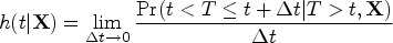
The use of the Cox proportional hazards model is ubiquitous in clinical and epidemiological research. ¹ The Cox model relates the logarithm of the hazard function to a linear combination of explanatory variables (or functions derived from the explanatory variables such as higher-order terms or interactions): $\log (h(t|X_1,\dots ,X_p))=\log (h_0(t))+{\beta }_1{X}_1+\cdots +{\beta }_p{X}_p$ , where t denotes time, $h(t|X_1,\dots ,X_p)$ denotes the hazard function for a subject with covariates $X_1,\dots ,X_p$ , and $h_0(t)$ denotes the baseline hazard function for an individual whose covariates are all equal to zero. The conventional measure of association for the Cox model is the hazard ratio: the ratio of the hazard function between two individuals with different sets of covariates. For the jth regression coefficient, $\exp ({\beta }_j)$ is the hazard ratio comparing the hazard function between two individuals whose value of the jth covariate differs by one unit and for whom the remaining p-1 covariates are equal between the two individuals.

When the Cox model assumes a linear relation between a given continuous covariate (e.g. age) and the log-hazard of the outcome then there is a single hazard ratio comparing any two individuals whose value of the given continuous variable differs by one unit. Thus, using the example of age, the hazard ratio comparing the hazard of the outcome between a 31- and a 30-year-old is the same as the hazard ratio comparing the hazard of the outcome between an 81- and an 80-year-old. While assuming a linear relation between a continuous variable and the log-hazard of the outcome results in an easily interpretable uniform hazard ratio, the assumption of linearity has been criticized by several authors.^2–4 In many clinical and epidemiological settings, the assumption of linearity may not be realistic. Different methods, including restricted cubic splines (RCS) and fractional polynomials, have been proposed to allow for the modeling of nonlinear relations between a continuous covariate and the outcome in a regression model.^2,4

An advantage to allowing for nonlinear relations between a continuous variable and the log-hazard of the outcome in a Cox model is that the assumption of linearity may be unrealistic in some settings. Thus, incorporating nonlinear relations may result in a regression model that more accurately describes the relation between covariates and the hazard of the outcome. A potential disadvantage to allowing for a nonlinear relation is that it becomes more difficult to describe the nature of relation between the given continuous predictor variable and the log-hazard of the outcome.

The objective of the current paper is to explore different graphical methods for describing the relation between a continuous variable and a time-to-event outcome when using restricted cubic splines with a Cox proportional hazards model to model the relation. The methods described in this article assume that preliminary analyses have led the analyst to allow for a nonlinear relationship between a continuous covariate and the log-hazard of the outcome. The presented methods will allow for communicating the nature of the relationship between the continuous covariate and the outcome. The article is structured as follows: in section 2, we propose four graphical methods to describe the relation between a continuous predictor variable and the outcome when using RCS with a Cox regression model. In section 3, we illustrate the application of these methods using data on patients hospitalized with heart failure (HF). In section 4, we present the results of mathematical derivations motivated by the findings of our case study. Finally, in section 5, we summarize our findings and present them in the context of the existing literature.

2 Graphical methods for illustrating relations between a continuous variable and outcomes when using restricted cubic splines with a Cox regression model

2.1 Restricted cubic splines

Restricted cubic splines require the specification of k knots. Harrell suggests that the knots be placed at equidistant percentiles of the continuous variable (thus, with four knots, one would place the knots at the 5th, 35th, 65th, and 95th percentiles of the continuous variable). ² RCS allows for a smooth nonlinear curve that is linear in the tails (to the left of the first knot and to the right of the last knot) and that is a cubic polynomial between adjacent knots such that the function is continuous and smooth at the knots where two cubic polynomials meet. An RCS with k knots requires the specification of k−1 variables that are themselves functions of the given continuous variable and the knots, with one of the variables being equal to the original continuous variable. These k−1 variables are then entered as explanatory or independent variables in a regression model.

2.2 Notation and background on survival analysis

Let T denote the event time. The hazard function, which is a function of time (denoted by t), is defined as:

$$h(t|\mathbf{\text{X}})=\underset{\mathrm{\Delta }t\to 0}{lim}\frac{Pr(t<T\le t+\mathrm{\Delta }t|T>t,\mathbf{\text{X}})}{\mathrm{\Delta }t}$$

(1)

where $\mathbf{\text{X}}$ denotes a vector of covariates. The hazard function is often interpreted as the instantaneous rate of the occurrence of the outcome. The cumulative hazard function is defined as $H(t|\mathbf{\text{X}})={\int }_0^{t}h(t|\mathbf{\text{X}})\text{d}t$ , while the survival function is defined as $S(t|\mathbf{\text{X}})=Pr(T>t|\mathbf{\text{X}})$ . The survival function and the cumulative hazard function are related as follows: $S(t|\mathbf{\text{X}})=e^{-H(t|\mathbf{\text{X}})}$ . The cumulative incidence function is defined as $F(t|\mathbf{\text{X}}\text{) = }1-S(t|\mathbf{\text{X}})=Pr(T\le t|\mathbf{\text{X}})$ .

The Cox proportional hazards model relates the logarithm of the hazard function to a linear combination of explanatory variables:

$$\log (h(t|\mathbf{\text{X}}))=\log (h_0(t))+\mathit{\beta }\mathbf{\text{X}}$$

(2)

where $h_0(t)$ is the baseline hazard function, which denotes the hazard function for an individual whose covariates are all equal to zero, and $\mathit{\beta }$ the associated vector of regression coefficients. Formula (2) is written in linear form where the log-hazard function is a linear function of the covariates. One can also write the Cox model in multiplicative form:

$$h(t|\mathbf{\text{X}})=h_0(t)e^{\mathit{\beta }\mathbf{\text{X}}}$$

(3)

The Cox model does not require the specification of a parametric distribution for the baseline hazard function or for the distribution of event times. Either the Breslow estimator or the Kalbfleisch and Prentice estimator can be used to obtain an estimate of the baseline hazard or survival function.^5–7 Using the fitted model, one can compute the survival function for any covariate pattern: $S(t|\mathbf{\text{X}})=S_0{(t)}^{\exp (\mathbf{\text{X}}\mathit{\beta })}$ where $S_0(t)$ denotes the baseline survival function.

2.3 Graphical methods for displaying the relation between a continuous covariate and the outcome when using a Cox proportional hazards model with restricted cubic splines

We describe four graphical methods for illustrating the relation between a continuous covariate and the outcome when using a Cox regression model with RCS. For the sake of simplifying the mathematical expressions, we assume that the model contains a single continuous variable and that this variable is modeled using RCS. The four methods are easily generalizable to multivariable models.

First, one can select a given value of the continuous covariate as the reference level. Candidates include the minimum value of the continuous variable or the mean or median value. In the case study below this will be the minimum value or the average value, depending on the variable. We denote this quantity by $x_{\text{ref}}$ . Using the fitted model, one estimates the value of the hazard function at $X=x$ and at $X=x_{\text{ref}}$ : $h(t|x)=h_0(t)e^{\mathit{\beta }f(\mathbf{\text{x}})}$ and $h(t|x_{\text{ref}})=h_0(t)e^{\mathit{\beta }f({\mathbf{\text{x}}}_{\text{ref}})}$ , where f() is the function that is used to represent X using RCS. Then, the hazard ratio comparing $X=x$ with $X=x_{\text{ref}}$ is equal to $\text{HR}(x;x_{\text{ref}})=\frac{h_0(t)e^{\mathit{\beta }f(x)}}{h_0(t)e^{\mathit{\beta }f(x_{\text{ref}})}}=e^{{}^{\mathit{\beta }(f(x)-f(x_{\text{ref}}))}}$ . One can then plot $\text{HR}(x;x_{\text{ref}})$ against x across the observed range of X in the sample. The resultant graph allows one to visualize the relative change in the instantaneous hazard of the outcome comparing $X=x$ with $X=x_{\text{ref}}$ .

Second, one can estimate the cumulative incidence function at a clinically meaningful value of t, denoted as $t_0$ (e.g. 1 year or 10 years) for each value of X: $F(t_0|x)=1-S_0(t_0{)}^{\exp (\mathit{\beta }f(x))}$ . One can then plot $F(t_0|x)$ against x to illustrate the relation between X and the cumulative incidence of the outcome at time $t_0$ . A limitation of this approach is that if the Cox regression model incorporates more than one variable (e.g. at least one variable in addition to the variable whose relation we want to describe graphically), there will be a different cumulative incidence function for each covariate pattern. One analytic option is to compute the cumulative incidence function when the other covariates are set to their median values. Alternatively, one could compute the cumulative incidence function at several clinically meaningful sets of covariates.

Third, one can compute the instantaneous hazard of the outcome at each value of $X=x$ at a specified time $t_0$ : $h(t_0|x)=h_0(t_0)e^{\mathit{\beta }f(x)}$ . As with the second method, one can plot the instantaneous hazard function at time $t_0$ against the value of x. As with the second method, when one incorporates additional variables in the Cox regression model, one would need to decide on the values of the other variables at which the hazard function is calculated.

The fourth approach is similar to the third, but one computes and plots the cumulative hazard function rather than the instantaneous hazard function. As with the second and third methods, one needs to decide on the values of the other variables at which the cumulative hazard function is calculated.

3 Case study

3.1 Data

We used data from a previous study that used 12,705 adults who presented to hospital emergency departments (EDs) in Ontario, Canada with a primary diagnosis of HF. ⁸ The study outcome for this case study was time to all-cause mortality, with subjects being followed for up to 2 years after ED presentation. Subjects were censored after 2 years if death had not yet occurred. Of the 12,705 patients, 35.4% died within 2 years of ED presentation.

3.2 Statistical analyses

We fit a Cox regression model in which the hazard of death was regressed on the following variables measured at the time of ED presentation: age, systolic blood pressure, heart rate, oxygen saturation, serum creatinine, serum potassium, sex, transport to hospital by emergency medical services, use of metolazone, previous myocardial infarction, previous heart failure, coronary artery bypass graft surgery, percutaneous coronary intervention, diabetes mellitus, hypertension, active and metastatic cancer, unstable angina, stroke, functional disability, cardiopulmonary respiratory failure and shock, pneumonia, chronic obstructive pulmonary disease, protein calorie malnutrition, dementia, trauma, major psychiatric disorders, peripheral vascular disease, renal failure, chronic liver disease, chronic atherosclerotic disease, and valvular disease. The first five variables were continuous, serum potassium was a three-level categorical variable, while the remaining variables were dichotomous. In the regression model, we used RCS to model the relation between the log-hazard of death and age, systolic blood pressure, heart rate, and creatinine. For age and creatinine, we used five knots, for systolic blood pressure we used four knots, and for heart rate we used three knots. Knots were placed at equidistant percentiles of the given variable, as suggested by Harrell. ² When we used fewer than five knots, the decision to do so was influenced by the distribution of the given variable: in these instances, some of the recommended percentiles coincided.

To illustrate the methods described in section 2, we focused on four continuous variables: age, systolic blood pressure, heart rate, and creatinine. For each of these four variables, we used the four methods described in section 2 to illustrate graphically the nature of the relation between the continuous variable and mortality. For the first method that requires a reference value of the given variable for the calculation of hazard ratios, we used the minimum observed value for age and heart rate (the minimums were 20 years and 80 beats per minute, respectively). For systolic blood pressure and creatinine, the minimums were 0 and 0.000226, respectively. As these values are not clinically plausible for living patients, we used the sample mean as the reference value for these two variables (the sample means of systolic blood pressure and creatinine were 141 and 1.16, respectively). For the second through fourth methods that require the specification of a time at which to estimate the cumulative incidence function, the hazard function, or the cumulative hazard function, we specified that $t_0=365$ days or 1 year. Furthermore, for these three methods that also require the specification of a covariate pattern at which to estimate these functions, we set all the other model covariates to their median value.

Figure 1.

Relationship between age and mortality.

3.3 Results

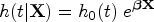
The relation between age and mortality is described in Figure 1, which consists of four panels, one for each of the graphical methods described in section 2. The shape of the curve was qualitatively similar across the four panels. In each of the four panels one observes an initial gradual increase in the “risk” of death with increasing age. However, from approximately age 80 onwards, there is a larger increase in “risk” of death with increasing age. Note that we use the term “risk” in a generic and nontechnical sense, thereby allowing us to describe all four panels simultaneously. “Risk”’ can be interpreted, depending on the setting, as the relative hazard of death, the probability of death within 1 year, the instantaneous hazard of death at 1 year, or the cumulative hazard of death within 1 year.

Figure 2.

Relationship between systolic blood pressure and mortality.

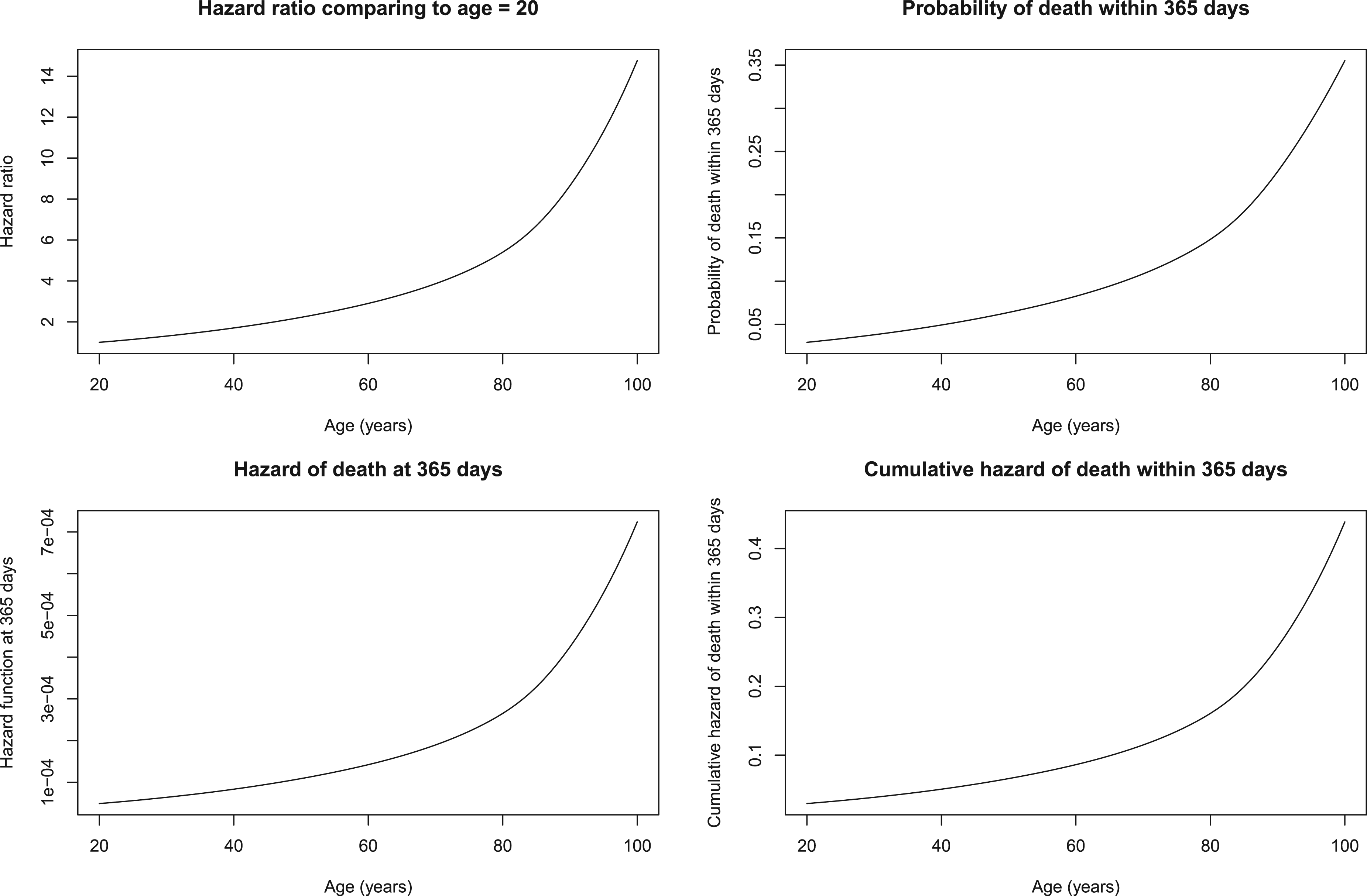
The relation between systolic blood pressure and mortality is described in Figure 2. As with age, the shape of the curve is qualitatively similar across the four methods. In each panel we observe that the “risk” of death decreases with increasing blood pressure. Furthermore, the relation with blood pressure is approximately linear.

Figure 3.

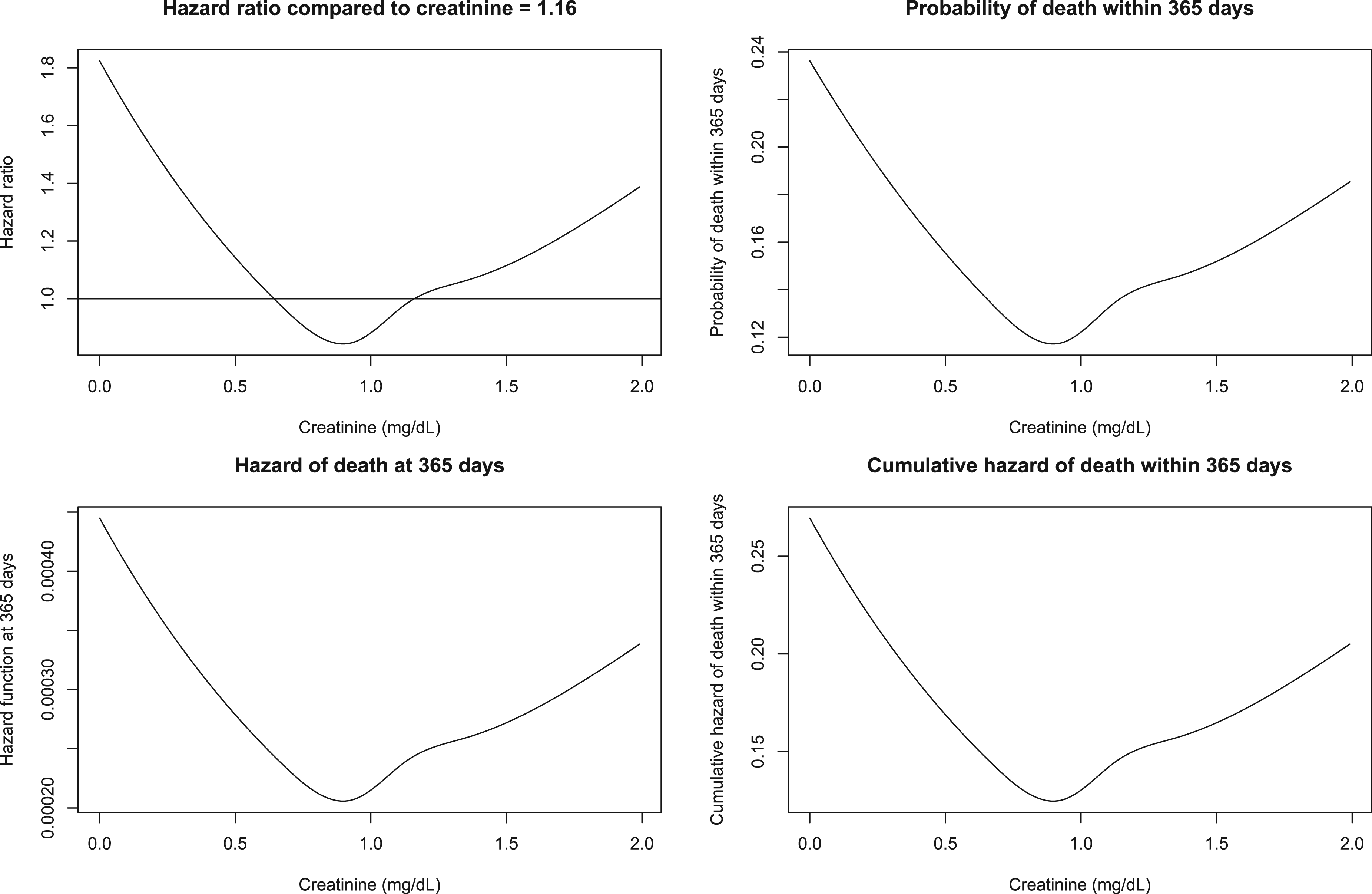
Relationship between creatinine and mortality.

The relation between creatinine and mortality is described in Figure 3. As with age and blood pressure, the shape of the curve is qualitatively similar across the four methods. In each panel we observe that the “risk” of death initially decreases with increasing creatinine, then reaches a nadir when creatinine is approximately 0.9, and then subsequently increases with increasing creatinine.

Figure 4.

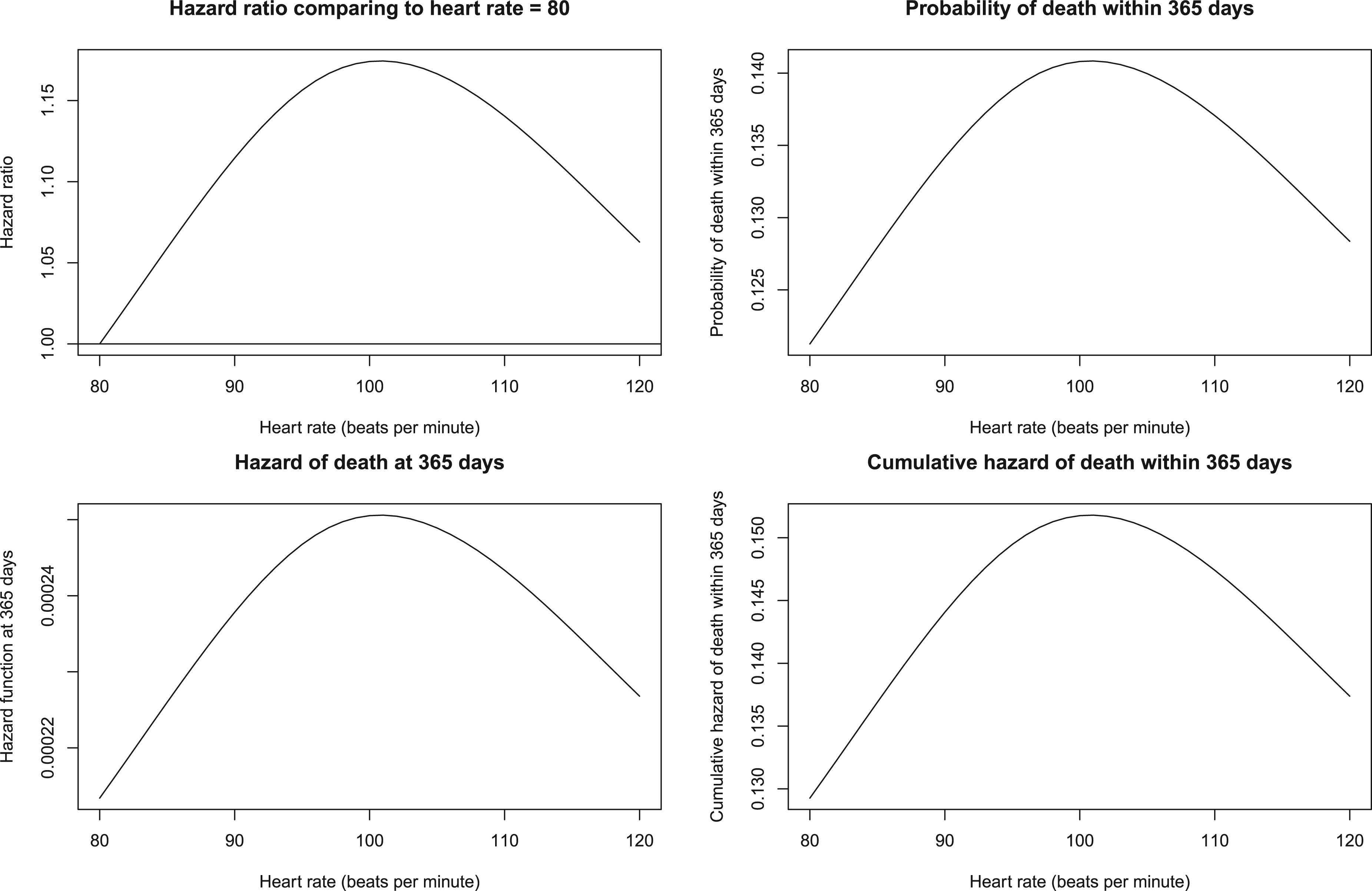
Relationship between heart rate and mortality.

Finally, the relation between heart rate and mortality is described in Figure 4. As with the other three variables, the shape of the curve is qualitatively similar across the four methods. In each panel we observe that the “risk” of death initially increases with increasing heart rate, then reaches a maximum when heart rate is approximately 100, and then subsequently decreases with increasing heart rate.

4 Mathematical derivations

Motivated by the qualitatively similar relation between a given continuous variable and the outcome across the four graphical methods that we observed above, we conducted mathematical derivations to demonstrate the generalizability of these observations. For simplicity, in the derivations that follow, we assume that the Cox model incorporates a single continuous variable, denoted by X, using RCS with k knots. Thus, within each interval defined by the knots, the continuous variable can be represented using a cubic polynomial. The relation will be linear in the tails; however, linearity is a special case of a cubic polynomial.

4.1 Plot of hazard ratios comparing each level of X with a reference level of X

Within an interval determined by adjacent knots (or in the interval to the left of the lower knot or in the interval to the right of the upper knot), the Cox model can be written as: $h(t|X)=h_0(t)e^{a_0+a_{1}x+a_2{x}^2+a_3{x}^3}$ for X in the given interval. If $X=x_{\text{ref}}$ is in a different interval, we write the Cox model in the interval containing $X=x_{\text{ref}}$ as: $h(t|X)=h_0(t)e^{b_0+b_{1}x+b_2{x}^2+b_3{x}^3}$ .

The hazard ratio comparing the hazard of the outcome at $X=x$ and $X=x_{\text{ref}}$ is equal to $\text{HR}(x;x_{\text{ref}})=\frac{h_0(t)e^{a_0+a_{1}x+a_2{x}^2+a_3{x}^3}}{h_0(t)e^{b_0+b_1{x}_{\text{ref}}+b_2{x}_{\text{ref}}^2+b_3{x}_{\text{ref}}^3}}=e^{a_0+a_{1}x+a_2{x}^2+a_3{x}^3-b_0-b_1{x}_{\text{ref}}-b_2{x}_{\text{ref}}^2-b_3{x}_{\text{ref}}^3}$ . Note that this is a function of X and that $x_{\text{ref}}$ is a constant. Because $x_{\text{ref}}$ is a constant, the derivative of this expression is equal to: $\frac{d\text{HR}(x;x_{\text{ref}})}{dx}=(e^{a_0+a_{1}x+a_2{x}^2+a_3{x}^3-b_0-b_1{x}_{\text{ref}}-b_2{x}_{\text{ref}}^2-b_3{x}_{\text{ref}}^3})(a_1+2a_{2}x+3a_3{x}^2)$ .

The first term in the derivative is strictly positive. Thus, the sign of the derivative will be determined solely by the second term $(a_1+2a_{2}x+3a_3{x}^2)$ . The curve describing the hazard ratio relative to $X=x_{\text{ref}}$ will be decreasing when this term is negative and will be increasing when this term is positive. Note that the upper and lower tails reduce to a linear function and that a₂ and a₃ will be equal to 0.

In the derivative above, the sign of the derivative will be determined only by the term $(a_1+2a_{2}x+3a_3{x}^2)$ . Importantly, this term does not include $x_{\text{ref}}$ . Thus, the choice of reference level will not change the intervals in which the curve was increasing and the intervals in which the curve was decreasing. Furthermore, the second derivative is equal to $\frac{{\mathrm{\partial }}^2\text{HR}(x;x_{\text{ref}})}{\mathrm{\partial }{x}^2}=(e^{a_0+a_{1}x+a_2{x}^2+a_3{x}^3-b_0-b_1{x}_{\text{ref}}-b_2{x}_{\text{ref}}^2-b_3{x}_{\text{ref}}^3})({(a_1+2a_{2}x+3a_3{x}^2)}^2+2a_2+6a_{3}x)$ . The sign of the second derivative is determined only by the term $({(a_1+2a_{2}x+3a_3{x}^2)}^2+2a_2+6a_{3}x)$ , which does not include $x_{\text{ref}}$ . As with the first derivative, the choice of the reference level will not change the intervals in which the second derivative is positive and the intervals in which the second derivative is negative. The choice of reference level will not affect the regions in which the curve is concave up and the intervals in which it is concave down. Similar, it will not affect the inflection points of the resultant curve. Thus, while the choice of reference level may result in the curve being shifted upwards or downwards, the choice of reference level should not affect the general shape of the curve. In the case study above, for two of the variables (systolic blood pressure and creatinine), we chose the sample mean as the reference value instead of the sample minimum. While this might have resulted in the curve being shifted upwards or downwards, it did not affect the general shape of the curve.

4.2 Plot of the cumulative incidence of the outcome at a specific time against X

Within an interval defined by adjacent knots, the cumulative incidence of the outcome at time t₀ is defined as $F(t_0|x)=1-S_0(t_0{)}^{\exp (a_0+a_{1}x+a_2{x}^2+a_3{x}^3)}$ . Since $S_0(t_0)$ is a constant, the derivative of this expression is $\frac{dF(t_0|x)}{dx}=(\log (S_0(t_0)))(-e^{a_0+a_{1}x+a_2{x}^2+a_3{x}^3})(S_0{(t_0)}^{\exp (a_0+a_{1}x+a_2{x}^2+a_3{x}^3)})(a_1+2a_{2}x+3a_3{x}^2)$ . The first term is strictly negative since the survival function is a strictly <1. Similarly, the second term is strictly negative, while the third term is strictly positive. Thus, the sign of the derivative will be determined solely by the last term $(a_1+2a_{2}x+3a_3{x}^2)$ . The curve describing the cumulative incidence function at time t₀ will be decreasing when this term is negative and will be increasing when this term is positive. Note that the upper and lower tails reduce to a linear function and that a₂ and a₃ will be equal to 0.

4.3 Plot of the hazard function of the outcome at a specific time against X

Within an interval determined by adjacent knots (or in the interval to the left of the lower knot or the interval to the right of the upper knot), the hazard function can be written as $h(t|x)=h_0(t)e^{a_0+a_{1}x+a_2{x}^2+a_3{x}^3}$ for x in the given interval. The derivative of this function at time $t_0$ is $\frac{dh(t_0|x)}{dx}=(h_0(t_0))(e^{a_0+a_{1}x+a_2{x}^2+a_3{x}^3})(a_1+2a_{2}x+3a_3{x}^2)$ . The first component is strictly positive as the hazard function is based on a probability and thus cannot be 0 or negative. Similarly, the second component is strictly positive. Thus, the sign of the derivative will be determined solely by the third component $(a_1+2a_{2}x+3a_3{x}^2)$ . The curve describing the hazard function at time t₀ as a function of X will be decreasing when this term is negative and will be increasing when this term is positive. Note that the upper and lower tails reduce to a linear function and that a₂ and a₃ will be equal to 0.

4.4 Plot of the cumulative hazard function of the outcome at a specific time against X

Within an interval determined by adjacent knots (or in the interval to the left of the lower knot or the interval to the right of the upper knot), the cumulative hazard function at time $t_0$ can be written as $H(t_0|x)={\int }_0^{t_0}h(t|x)dt={\int }_0^{t_0}{h}_0(t)e^{a_0+a_{1}x+a_2{x}^2+a_3{x}^3}dt=e^{a_0+a_{1}x+a_2{x}^2+a_3{x}^3}{\int }_0^{t_0}{h}_0(t)dt$ for x in the given interval. The derivative of this expression is $\frac{dH(t_0|x)}{dx}=(h_0(t_0))(e^{a_0+a_{1}x+a_2{x}^2+a_3{x}^3})(a_1+2a_{2}x+3a_3{x}^2)$ . The first component is strictly positive as the hazard function is based on a probability and thus cannot be 0 or negative. Similarly, the second component is strictly positive. Thus, the sign of the derivative will be determined solely by the third component $(a_1+2a_{2}x+3a_3{x}^2)$ . The curve describing the cumulative hazard function at time t₀ as a function of X will be decreasing when this term is negative and will be increasing when this term is positive. Note that the upper and lower tails reduce to a linear function and that a₂ and a₃ will be equal to 0.

Thus, for a given interval determined by adjacent knots (or in the lower and upper tails), each of the four curves will be decreasing when $(a_1+2a_{2}x+3a_3{x}^2)$ is negative and will be increasing when $(a_1+2a_{2}x+3a_3{x}^2)$ is positive. Thus, the four curves will be simultaneously increasing or simultaneously decreasing. Consequently, the shape of the four curves will be similar to one another, in terms of regions in which each is increasing or decreasing.

In the above derivations, we assumed that the Cox model included a single continuous variable represented using RCS. If there were additional covariates in the model, the derivative of the linear predictor for these covariates with respect to X would be 0, resulting in identical conclusions.

5 Discussion

We described four methods to graphically describe the relation between a continuous covariate and the outcome when using a Cox proportional hazards model. These graphical methods allow investigators to provide a simple graphical description of the nature of the relation between a continuous covariate and the outcome. We demonstrated, both using a case study and mathematical derivations, that the four methods will result in qualitatively similar conclusions about the nature of the relation between the continuous covariate and the time-to-event outcome.

The methods that we have described assume that the analyst has decided to allow a nonlinear relationship between a continuous variable and the log-hazard of the outcome. This decision could be based on exploratory data analysis, results from previously published studies, or based on statistical practice. The methods that we have described are not intended to inform that decision. However, once the decision has been made to allow for nonlinear relationships, the methods that we have described allow for a graphical communication of the nature of the relationship between the variable and the risk of the outcome.

There are relative advantages and disadvantages to the four methods. The first method computes the hazard ratio comparing the relative change in the hazard of the outcome for each value of the continuous covariate compared to the hazard of the outcome for a specified reference level of the continuous covariate. An advantage to this method is that it uses the hazard ratio, which is the common measure of association when using the Cox model. A second advantage to this approach is that, unlike the other three methods, it does not require estimation of the baseline hazard function, which can be considered a nuisance parameter. A third advantage of this approach is that the general shape of the curve is independent of the choice of reference level used for computing hazard ratios. A disadvantage of this approach is that the curve is a relative curve, with the hazard at a given value of the covariate being compared to the hazard at the reference value of the covariate. A second disadvantage to this approach is that one must specify the reference value of the variable. However, as demonstrated above, the choice of reference level will not affect the general shape of the curve. The other three methods describe the relation between the continuous covariate and the cumulative incidence, the hazard function, and the cumulative hazard function. A disadvantage of each of these three methods is that each requires the specification of a time at which the cumulative incidence, the hazard, and the cumulative hazard are computed. A second disadvantage of these three methods is that each requires the specification of a covariate pattern at which each of these functions is evaluated (e.g. the model covariates are set to the cohort median). However, the shape of the curve would be similar regardless of the covariate pattern chosen, with the resultant curve shifted upwards or downwards. A third disadvantage of these three methods is that each requires estimation of either the baseline hazard function or the baseline survival function, which are considered nuisance parameters in the Cox model. An advantage to these three methods is that each reports the absolute measure of association rather than a relative measure of association. A limitation of the method that reports the relationship between the covariate and the hazard of the outcome at a specific time is that the hazard function is defined as a limit. While the hazard function can be estimated or approximated, the reported value may vary across estimation procedures. If different estimation procedures are used, this may cause problems when comparing graphical results for this method across studies. In the case study, for all four variables, both the hazard of death at 365 days and the cumulative hazard of death within 365 days were strictly between 0 and 1 for all values of each of the four variables. A limitation of the two methods based on these quantities is that readers who lack familiarity with methods for survival analysis may be tempted to incorrectly assign a probabilistic interpretation to these quantities. Similarly, when reporting the cumulative hazard of the outcome, readers need to be aware that a ratio of cumulative hazards is not a reliable proxy for the hazard ratio.

The use of methods to allow for nonlinear relationship between continuous covariates and the log-hazard of the outcome are well established in survival analysis. The Cox model also allows for time-varying covariate effects, which relaxes the proportional hazards assumption and allows the hazard ratio to vary as a function of time. In a recent paper, we described a method to allow the regression coefficients to vary as a smooth function of time, by using restricted cubic splines to model the log-hazard ratio as a function time. ⁸ This method allowed for a graphical depiction of the hazard ratio as a smooth function of time. Future research is required to develop methods for combining these two approaches and producing a surface expressing the hazard ratio (or other any of the other measures) as a function of both the variable and time.

Our recommendation would be to use the method based on computing the hazard ratio comparing the relative change in the hazard of the outcome for each value of the continuous covariate compared to the hazard of the outcome for a specified reference level of the continuous covariate. This method does not require estimation of the baseline hazard function or of the baseline survival function. Furthermore, the general shape of the resultant curve is not influenced by the choice of reference level. However, we have demonstrated that qualitatively similar conclusions would be drawn regardless of the method used. This is an important message, since it allows for comparing results across different published studies that used different methods for describing the relationship between a given variable and the risk of the outcome. Thus, authors who have a different preference can implement that method knowing that it will produce qualitatively similar conclusions to those of the other methods.