Sage Journals: Discover world-class research

Abstract

We developed a command, csa2sls, that implements the complete subset averaging two-stage least-squares (CSA2SLS) estimator in Lee and Shin (2021, Econometrics Journal 24: 290–314). The CSA2SLS estimator is an alternative to the two-stage least-squares estimator that remedies the bias issue caused by many correlated instruments. We conduct Monte Carlo simulations and confirm that the CSA2SLS estimator reduces both the mean squared error and the estimation bias substantially when instruments are correlated. We illustrate the usage of csa2sls in Stata with an empirical application.

Keywords

st0732 csa2sls many instruments complete subset averaging two-stage least squares

1 Introduction

The two-stage least-squares (2SLS) estimator is one of the most widely used methods in applied economics. Theoretically, the optimal instrument can be achieved by the conditional mean function of the first-stage regression. However, in practice, practitioners working with a finite sample face a crucial question of how many instruments one should use, especially when there are many instruments available. This is partly due to the well-known tradeoff between bias and variance when the number of instruments increases. Donald and Newey (2001) show this point clearly with a higher-order Nagar expansion and propose choosing the optimal number of instruments that minimizes the mean squared errors (MSEs). Kuersteiner and Okui (2010) propose a model averaging approach for the first-stage regression and show that it achieves the optimal weight. These other approaches, however, require the practitioner to either know the order of importance among instruments (Donald and Newey 2001) because the method chooses the first few important instruments or estimate the optimal weights for the instruments (Kuersteiner and Okui 2010).

As an alternative, Lee and Shin (2021) propose a model-averaging approach that uses all size-k subsets of the set of available instruments in a cross-sectional regression model. This new approach is named the complete subset averaging two-stage least-squares (CSA2SLS) estimator. One advantage of the CSA2SLS estimator is that, because it uses all subsets, it does not require knowledge of the order of importance among instruments. Furthermore, averaging models using equal weights reduces potential efficiency loss in finite samples. This is because when estimated weights (instead of equal weights) are used, these become additional parameters in the model and therefore cause inefficiency when there are many models to be averaged.

We developed a command, csa2sls, that implements the CSA2SLS estimator. It selects the optimal number of subset size k that minimizes the approximate MSEs. Because the size of the complete subset grows at the order of 2 ^K , where K is the total number of instruments, CSA2SLS is computationally intensive. To alleviate such a computational burden, the command csa2sls includes options for subsampling and a fast but memory-intensive method.

The remainder of this article is organized as follows. Section 2 introduces the CSA2SLS estimator in Lee and Shin (2021). Section 3 explains the command csa2sls. Section 4 shows results from Monte Carlo experiments that numerically illustrate how the CSA2SLS estimator alleviates some of the issues that arise from many instruments. Section 5 provides an empirical application of csa2sls. Section 6 concludes.

2 CSA2SLS estimator

In this section, we explain the key idea of the CSA2SLS estimator in Lee and Shin (2021). Heuristically speaking, we estimate the first-stage predicted value by model averaging and apply the 2SLS estimation with those predicted values. Given a total of K instruments, we consider all subsets composed of k instruments. We compute a simple average of predicted values across models, and the 2SLS estimator follows immediately. The optimal k is selected by minimizing the approximate MSEs criterion, which will be explained in detail below.

To be concrete, consider the following model generated from an independent and identically distributed sample:

\begin{array}{l} y_{i} = Y_{i}^{'} β_{y} + x_{1 i}^{'} β_{x} + ϵ_{i} = X_{i}^{'} β + ϵ_{i} \\ X_{i} = [\begin{matrix} Y_{i} \\ x_{1 i} \end{matrix}] = f (z_{i}) + u_{i} = [\begin{matrix} E (Y_{i} ∣ z_{i}) \\ x_{1 i} \end{matrix}] + [\begin{matrix} η_{i} \\ 0 \end{matrix}], i = 1, . . ., N \end{array}

where y_i is a scalar outcome variable, Y _i is a d ₁ × 1 vector of endogenous variables, x ₁ _i is a d ₂ × 1 vector of included exogenous variables, z _i is a vector of exogenous variables (including x ₁ _i ), f(·) is an unknown function of z, and ϵ_i and u _i are error terms uncorrelated with z _i . Finally, η _i denotes an error term when we project the endogenous regressor Y _i into the space of exogenous variable z _i . Note that E( η _i| z _i ) = 0 by construction.

Let y = (y ₁ ,…, y_N )′, ϵ = (ϵ ₁ ,…, ϵ_N )′, X = (X ₁ ,…, X _N )′, f = (f ₁ ,…, f _N )′, and U = (u ₁ ,…, u _N )′, where f _i = f(z _i ). The set of instruments has the form Z _K,i ≡ {ψ ₁(z _i ),…, ψ_K (z _i ), x ₁ _i }′, where ψ_k ’s are functions of z _i such that Z _K,i is the collection of (K + d ₂) instruments. Note that the total number of instruments K can increase as N → ∞. We suppress the dependency of K on N for notation simplicity. Let Z _K = (Z _K, ₁ ,…, Z _K,N )′ be the collection of Z _K,i .

Let M be the number of subsets (or models) with k instruments:

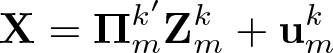
M = (\begin{matrix} K \\ k \end{matrix}) = \frac{K!}{k! (K - k)!}

We also suppress the dependency of M on K and k. Let m ∊ {1,…, M} be an index of each model and $z_{m, i}^{k}$ be a vector of instruments in model m. Then the first-stage regression of model m can be written as

X = Π_{m}^{k^{'}} Z_{m}^{k} + u_{m}^{k}

The average predicted value of X is

\hat{X} = \frac{1}{M} \sum_{m = 1}^{M} Z_{m}^{k} {\hat{Π}}_{m}^{k}

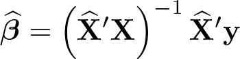
where ${\prod^{^}}_{m}^{k}$ is the ordinary least-squares (OLS) estimator of $\prod_{m}^{k}$ . Then the CSA2SLS estimator is defined as

\hat{β} = {(\hat{X}' X)}^{- 1} \hat{X}' y

Using the projection matrices, we can also write the CSA2SLS estimator as a one-step procedure,

\hat{β} = {(X^{'} P^{'} X)}^{- 1} X^{'} P^{k} y

where $P^{k} = M^{- 1} \sum_{m = 1}^{M} P_{m}^{k}$ with $P_{m}^{k} = Z_{m}^{k} {(Z_{M}^{K^{'}} Z_{m}^{k})}^{- 1} Z_{M}^{K^{'}}$ .

The optimal subset size k is chosen by minimizing the approximate MSE. Let $\tilde{β}$ be a preliminary estimator and $\tilde{ϵ} = y - X \tilde{β}$ . The fitted value of f is given as

\tilde{f} = {\tilde{Z}}^{k} {({\tilde{Z}}^{k'} {\tilde{Z}}^{k})}^{- 1} {\tilde{Z}}^{k'} X

where ${\tilde{Z}}^{k}$ consists of exogenous variables plus the preliminary selection of instruments as described above. Let ${\tilde{P}}_{Z} = {\tilde{Z}}^{k} {({\tilde{Z}}^{k'} {\tilde{Z}}^{k})}^{- 1} {\tilde{Z}}^{k'}$ . The residual matrix is denoted by $\tilde{u} = X - \tilde{f}$ . Define $\tilde{H} = {\tilde{f}}^{'} \tilde{f} / N, {\tilde{σ}}_{ϵ}^{2} = {\tilde{ϵ}}^{'} \tilde{ϵ} / N$ , ${\tilde{σ}}_{u ϵ} = {\tilde{u}}^{'} \tilde{ϵ} / N, {\tilde{σ}}_{λ ϵ} = {\tilde{λ}}^{'} {\tilde{H}}^{- 1} {\tilde{σ}}_{u ϵ}$ , and ${\tilde{Σ}}_{u} = {\tilde{u}}^{'} \tilde{u} / N$ . Then the sample counterpart of the approximate MSE is given by

{\hat{S}}_{λ} (k) = {\tilde{σ}}_{λ ϵ}^{2} \frac{k^{2}}{N} + {\tilde{σ}}_{ϵ}^{2} ({\tilde{λ}}^{'} {\tilde{H}}^{- 1} {\tilde{e}}_{f}^{k} {\tilde{H}}^{- 1} \tilde{λ} - {\tilde{λ}}^{'} {\tilde{H}}^{- 1} {\tilde{ξ}}_{f}^{k} {\tilde{H}}^{- 1} {\tilde{ξ}}_{f}^{k} {\tilde{H}}^{- 1} \tilde{λ})

where

\begin{array}{l} {\tilde{e}}_{f}^{k} = \frac{X^{'} {(I - P_{k})}^{2} X}{N} + {\tilde{Σ}}_{u} [\frac{2 k - tr {{(P^{k})}^{2}}}{N}] \\ {\tilde{ξ}}_{f}^{k} = \frac{X^{'} {(I - P_{k})}^{2} X}{N} + {\tilde{Σ}}_{u} \frac{k}{N} - {\tilde{Σ}}_{u} \\ {\tilde{σ}}_{λ ϵ}^{2} = {({\tilde{λ}}^{'} {\tilde{H}}^{- 1} {\tilde{σ}}_{λ ϵ})}^{2} \end{array}

The preliminary estimator $\tilde{β}$ can be estimated either by using Mallow’s two-step criterion or by adopting the one-step method. See Lee and Shin (2021) for details.

3 The csa2sls command

3.1 Syntax

The syntax for the command is as follows:

csa2sls depvar [varlist1] ( varlist2 = varlist_iv ) [if] [in] [, noconstant

hasconstant onestep r( # ) vce( vcetype ) level( # ) first small large

noheader depname( depname ) perfect]

varlist1 is the list of exogenous variables. varlist2 is the list of endogenous variables. varlist_iv is the list of exogenous variables used with varlist1 as instruments for varlist2.

3.2 Options

noconstant; see [R] Estimation options.

hasconstant indicates that a user-defined constant or its equivalent is specified among the independent variables.

onestep allows the one-step preliminary method. The default is Mallow’s two-step criterion. See Lee and Shin (2021).

r( # ) specifies a positive integer for the maximum number of randomly selected subsets when the number of subsets is bigger than #. This is useful because the number of subsets depends exponentially on the number of instruments.

vce( vcetype ) specifies the type of standard error reported, which includes types that are robust to some kinds of misspecification (robust) and that allow for intragroup correlation (cluster clustvar). vce(unadjusted) specifies that an unadjusted (nonrobust) variance–covariance estimate matrix be used.

level( # ); see [R] Estimation options.

first requests that the first-stage regression results be displayed.

small requests that the degrees-of-freedom adjustment N/(N − k) be made to the variance–covariance matrix of parameters and that small-sample F and t statistics be reported, where N is the sample size and k is the number of parameters estimated. By default, no degrees-of-freedom adjustment is made, and Wald and z statistics are reported. Even with this option, no degrees-of-freedom adjustment is made to the weighting matrix when the generalized method of moments estimator is used.

large turns on the large-sample estimation program. When the sample size is large, the average projection matrices may require a large memory size. The large option must be turned on to avoid an insufficient memory issue. The default is not using this option.

noheader suppresses the display of the summary statistics at the top of the output, displaying only the coefficient table.

depname( depname ) specifies to substitute the dependent variable name.

perfect requests that csa2sls not check for collinearity between the endogenous regressors and excluded instruments, allowing one to specify “perfect” instruments. This option may be required when using csa2sls to implement other estimators.

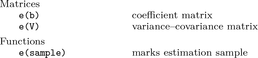
3.3 Stored results

csa2sls stores the following in e():

4 Monte Carlo experiments

In this section, we conduct Monte Carlo simulation studies focusing on the effect of correlated instruments. An independent and identically distributed sample (y_i, Y_i, z _i ) is generated from the following simulation design:

\begin{array}{l} y_{i} = β_{0} + β_{1} Y_{i} + ϵ_{i} \\ Y_{i} = π^{'} z_{i} + u_{i} \end{array}

where Y_i is a scalar endogenous regressor, (β ₀ , β ₁) is set to be (0, 0.1), and z _i is a K-dimensional vector of instruments generated from a multivariate normal distribution N(0, Σ _z ). The diagonal elements of Σ _z are set to be 1, and the off-diagonal elements are ρ_z . We set each element of π to be $\sqrt{0.1 / {K + K (K - 1) ρ_{z} (1 - 0.1)}}$ , where 0.1 is the R ² in the first-stage regression. The vector of error terms (ϵ_i, u_i ) follows a bivariate normal distribution whose means are zeros and variances are ones. The covariance between ϵ_i and u_i is set to be 0.9. In these simulation studies, K varies in {5, 10, 15, 20} and ρ_z varies in {0, 0.5, 0.9}. The sample size is set to be n = 100, and the results are from 1,000 replications.

Figure 1 summarizes the simulation results. We report the mean bias and MSE of CSA2SLS along with the performance of the OLS estimator and the 2SLS estimator. First, the CSA2SLS estimator reduces the bias substantially when instruments are correlated (ρ_z = 0.5, 0.9). As predicted by theory, the bias of 2SLS increases as K increases. Note that when instruments are independent (ρ_z = 0.0), the difference in the bias between the CSA2SLS estimator and the 2SLS estimator is small. Lee and Shin (2021) prove that the performance of CSA2SLS will be asymptotically equivalent to that of 2SLS when ρ_z = 0.

Second, the efficiency loss of CSA2SLS is modest. When instruments are correlated, CSA2SLS achieves lower MSEs when K ≥ 10. Like the bias, the MSE gap between CSA2SLS and 2SLS increases as K increases. It is also worthwhile to note that the MSE of CSA2SLS does not change much over different values of K. Finally, the OLS estimator performs the worst in these simulation designs.

To summarize, the CSA2SLS estimator shows a good finite sample performance as predicted by theory. We also observe the increased bias of 2SLS when there are many instruments. We recommend practitioners use the CSA2SLS estimator when they have many correlated instruments.

Figure 1.

Mean bias and MSE

5 Empirical illustration

In this section, we illustrate the usage of csa2sls with an empirical application. In this example, we revisit Berry, Levinsohn, and Pakes (1995) and estimate a logistic demand function for automobiles based on pooled cross-sectional data over different markets.

The model is specified as

\begin{array}{l} \log (S_{i}) - \log (S_{0}) = α_{0} P_{i} + X_{i}^{'} β_{0} + ϵ_{i} \\ P_{i} = Z_{i}^{'} δ_{0} + X_{i}^{'} ρ_{0} + u_{i} \end{array}

where S_i is the market share of product i with product 0 denoting the outside option, P_i is the endogenous price variable, X _i is a vector of included exogenous variables, and Z _i is a set of 10 instruments. The parameter of interest is α ₀, from which we can calculate the price elasticity of demand. Note that the optimal subset size k is 9 in this empirical example.

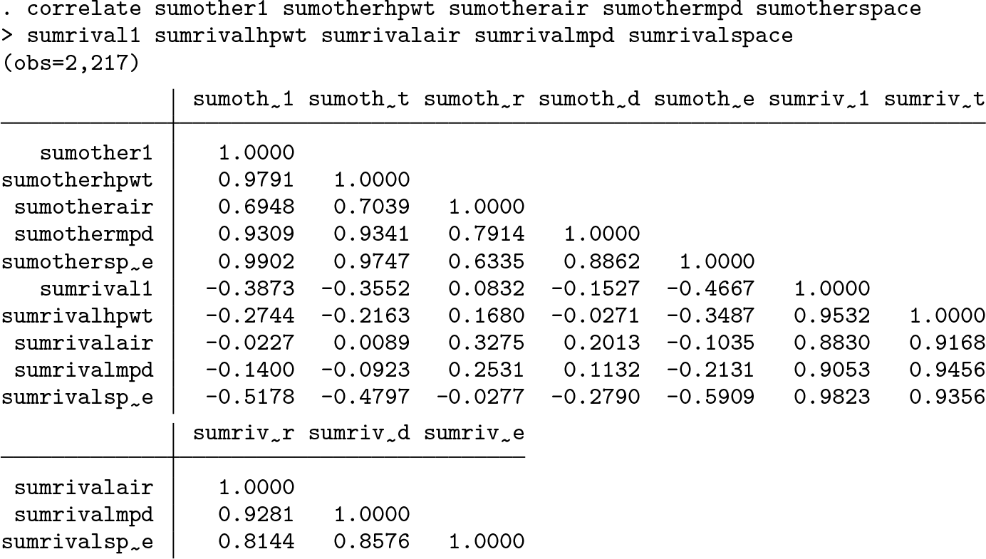
We also report correlation coefficients among the instruments. We can confirm that the instruments are divided into two groups and that each group’s instruments are highly correlated with each other.

6 Conclusion

In this article, we presented the CSA2SLS estimator and the corresponding command, csa2sls. The usage of csa2sls was illustrated with an empirical application. The Monte Carlo experiments show that 2SLS is biased when there are many instruments and that CSA2SLS outperforms 2SLS when instruments are correlated with each other. Because CSA2SLS is computationally intensive, an interesting future research question would be to develop a more efficient computation algorithm. An approach based on the stochastic gradient descent (see, for example, Lee et al. [2022]) can be a possible solution.

8 Programs and supplemental material

Supplemental Material, sj-zip-1-stj-10.1177_1536867X231212432 - csa2sls: A complete subset approach for many instruments using Stata

Supplemental Material, sj-zip-1-stj-10.1177_1536867X231212432 for csa2sls: A complete subset approach for many instruments using Stata by Seojeong Lee, Siha Lee, Julius Owusu and Youngki Shin in The Stata Journal

Footnotes

7 Acknowledgments

We would like to thank the editor and an anonymous reviewer for their valuable comments on this article and for their helpful feedback on the program code. Shin is grateful for partial support by the Social Sciences and Humanities Research Council of Canada (SSHRC-435-2021-0244).

8 Programs and supplemental material

To install the software files as they existed at the time of the publication of this article, type

References

Berry

Levinsohn

Pakes

. 1995. Automobile prices in market equilibrium. Econometrica 63: 841–890. https://doi.org/10.2307/2171802.

Donald

S. G.

Newey

W. K.

. 2001. Choosing the number of instruments. Econometrica 69: 1161–1191. https://doi.org/10.1111/1468-0262.00238.

Kuersteiner

Okui

. 2010. Constructing optimal instruments by first-stage prediction averaging. Econometrica 78: 697–718. https://doi.org/10.3982/ECTA7444.

Lee

Liao

Seo

M. H.

Shin

. 2022. Fast and robust online inference with stochastic gradient descent via random scaling. In Proceedings of the Thirty-Sixth International Joint Conference on Artificial Intelligence, 7381–7389. Buenos Aires, Argentina: AAAI Press.

Lee

Shin

. 2021. Complete subset averaging with many instruments. Econometrics Journal 24: 290–314. https://doi.org/10.1093/ectj/utaa033.