Nearly collinear robust procedures for 2SLS estimation

Abstract

Stata’s two-stage least-squares (2SLS) computation procedures are sensitive to near collinearity among regressors, allowing situations in which reported results depend upon factors as irrelevant as the order of the data and variables. This article illustrates this claim with the public-use data of Oreopoulos (2006, American Economic Review 96: 152–175), where the instrumented coefficient estimate can be made to vary between 0.012 and 30.0 in one specification by permuting the order of the variables. Different methods for improving the accuracy of 2SLS estimates are reviewed, and a Stata command for collinearity-robust 2SLS estimation is provided.

1 Introduction

Users of Stata regularly rely on its ability to weed out and drop perfectly collinear nuisance regressors. Problems arise, however, when regressors are not collinear enough to be flagged and dropped by Stata but are collinear enough to affect computational accuracy. When variables are nearly collinear, floating-point rounding errors in matrix operations are magnified, and reported results become sensitive to factors as econometrically irrelevant as the order of the data and variables. Sensitivity to collinearity is greater when conditioning on nuisance variables substantively affects point estimates, that is, precisely when otherwise irrelevant variables play essential roles in the regression by conditioning out potential bias. These issues are especially relevant for two-stage least-squares (2SLS) estimation, where the standard formula used by Stata’s ivregress command incorrectly assumes that the estimated inverse of the matrix of instrument inner products times the matrix itself is exactly equal to the identity matrix.

This article proceeds as follows: Section 2 lays out the canonical formula for 2SLS estimation and how its implicit assumption of zero computational error in matrix inversion can render estimates sensitive to irrelevancies such as the order of the data and variables. Section 3 illustrates the problem using the public-use data and instrumental-variables (IV) regressions of Oreopoulos (2006). Estimated 2SLS coefficients in that article using Stata’s ivreg or ivregress command are shown to be sensitive to econometrically irrelevant procedures, varying as much as from 0.012 to 30.0 in one specification through a simple reordering of variables. Section 4 reviews various computational methods for 2SLS estimation, and section 5 tests these, as well as the community-contributed commands ivreg2 (Baum, Schaffer, and Stillman 2002) and xtivreg2 (Schaffer 2005), on Oreopoulos’s data and a broad sample of published 2SLS regressions whose regressors are rotated to artificially increase collinearity. The community-contributed commands are found to be much less sensitive to near collinearity than Stata’s built-in commands but still orders of magnitude more sensitive than can be achieved by partitioning the 2SLS regression, which avoids cascading matrix inverse errors and produces minimal sensitivity to econometrically irrelevant procedures. Section 6 introduces pariv, a command that implements this collinearity-robust 2SLS estimation method, checks the sensitivity of results to the order of the data and variables, and reports the maximum R ² found in the regression of one instrument on the others. Section 7 concludes with suggestions for safer econometric and programming practice.

2 Typical 2SLS estimation methods

IV estimates are usually implemented using the canonical textbook representation of 2SLS. Following the notation of Stata’s help files, let

$y=Y{\beta }_1+X_1{\beta }_2+u=X\beta +u\hspace{0.17em}\text{and}\hspace{0.17em}Y=X_1{\Pi }_1+X_2{\Pi }_2+V=Z\Pi +V$

where y is the n × 1 vector of second-stage outcomes, Y the n × p matrix of endogenous regressors, X ₁ the n × k ₁ matrix of included instruments (exogenous regressors), X ₂ the n × k ₂ matrix of excluded instruments, and u and V the n × 1 and n × p vector and matrix of second and first-stage disturbances. The remaining (Greek) letters are vectors and matrices of parameters. Stata, as well as some of the toolboxes proffered online for users of MATLAB, estimates the second-stage coefficients using the formula ¹

$\widehat{\beta }={\left\{X^{\prime }Z{\left(Z^{\prime }Z\right)}^{-1}{Z}^{\prime }X\right\}}^{-1}{X}^{\prime }Z{\left(Z^{\prime }Z\right)}^{-1}{Z}^{\prime }y$

1

Under normal circumstances, (1) is equivalent to running the ordinary least-squares (OLS) regression of y on the projection of X on Z, $\widehat{\mathbf{X}}=Z{({\mathbf{Z}}^{\prime }\mathbf{Z})}^{-1}{\mathbf{Z}}^{\prime }\mathbf{X}$ . However, when Z is nearly collinear, (Z ′ Z) ^{− 1} as calculated using machine precision is not close to the true inverse of Z ′ Z, so the computed value of (Z ′ Z) ^{− 1}(Z ′ Z) differs substantially from the identity matrix, and (1) does not yield OLS coefficients. The error in the assumption that the computed value of (Z ′ Z) ^{− 1}(Z ′ Z) equals the identity matrix will vary with the order of the data, variables, and even the processor because these will affect the floatingpoint error in the sums Z ′ Z and the way in which these errors cumulatively affect the calculation of (Z ′ Z) ^{− 1}. Estimated coefficients can then become substantively sensitive to otherwise econometrically irrelevant procedures.

3 An illuminating example: Oreopoulos (2006)

Oreopoulos (2006) estimates the Mincerian return to schooling using IV based on variation induced by compulsory schooling laws in the United Kingdom and (to a much lesser extent) the United States and Canada. Oreopoulos’s IV specifications include quartic polynomials in the age of the respondent at the time labor income is reported or quartic polynomials in the birth cohort as exogenous regressors (that is, included instruments) or both. ² In all the U.K. IV samples estimating a Mincerian return, the R ² of the projection of age on age raised to the second through the fourth power or cohort year on cohort year raised to the second through the fourth power is always in excess of 0.999998. The use of dummy variables for age, birth cohort, region, region interacted with birth cohort, and year further increases collinearity, with the maximum R ² in the regression of one included instrument on the others lying above 0.99999989 in all Mincerian U.K. specifications. In sum, ancillary regressors, whose coefficients are not important enough to ever be reported, are highly collinear. Below, I focus on the U.K. IV estimates of the Mincerian return because these are by far the most sensitive.

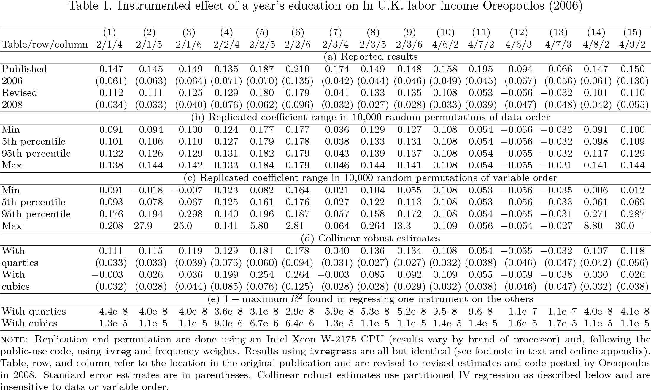
Panel (a) of table 1 lists all 15 IV-estimated U.K. Mincerian returns and associated standard errors published in tables in the article, as well as revised estimates posted on the American Economic Review data page in 2008 by Oreopoulos in response to reported difficulties in reproducing his results. In panel (b), I replicate his results using the data and specifications given in his 2008 public-use code while randomly varying the order of the data 10,000 times. As shown, the order of the data discernibly affects the estimated Mincerian return in most specifications, with max–min differences of 0.05 in a few cases. Panel (c) randomly permutes the order of the variables when entered in the regression. All estimated Mincerian returns are sensitive to this, with a max–min difference of up to 30. In all cases, the maximum and minimum coefficient estimates are associated with regressions in which Stata reports finite standard errors for the Mincerian return as well as for all other estimated coefficients (excluding variables that are dropped), and there is nothing in the results to alert the user to the fact that they are sensitive to what should otherwise be completely irrelevant procedures. With sample sizes in the thousands and dozens of dummies in some specifications, 10,000 random permutations barely scratch the surface of the N! possible permutations of the order of the data or variables, understating the actual max–min difference. Percentiles, however, are more accurately estimated with random sampling while providing a sense of the variation found in the typical permutation. As shown, the 5th to 95th percentile range of the estimated Mincerian return found in random permutations of variable order is in excess of 0.2 in three specifications and of 0.1 in five. ³

Table 1.

Instrumented effect of a year’s education on ln U.K. labor income Oreopoulos (2006)

Table/row/column	(1)2/1/4	(2)2/1/5	(3)2/1/6	(4)2/2/4	(5)2/2/5	(6)2/2/6	(7)2/3/4	(8)2/3/5	(9)2/3/6	(10)4/6/2	(11)4/7/2	(12)4/6/3	(13)4/7/3	(14)4/8/2	(15)4/9/2
(a) Reported results
Published	0.147	0.145	0.149	0.135	0.187	0.210	0.174	0.149	0.148	0.158	0.195	0.094	0.066	0.147	0.150
2006	(0.061)	(0.063)	(0.064)	(0.071)	(0.070)	(0.135)	(0.042)	(0.044)	(0.046)	(0.049)	(0.045)	(0.057)	(0.056)	(0.061)	(0.130)
Revised	0.112	0.111	0.125	0.129	0.180	0.179	0.041	0.133	0.135	0.108	0.053	−0.056	−0.032	0.101	0.110
2008	(0.034)	(0.033)	(0.040)	(0.076)	(0.062)	(0.096)	(0.032)	(0.027)	(0.028)	(0.033)	(0.039)	(0.047)	(0.048)	(0.042)	(0.055)
(b) Replicated coefficient range in 10,000 random permutations of data order
Min	0.091	0.094	0.100	0.124	0.177	0.177	0.036	0.129	0.127	0.108	0.054	−0.056	−0.032	0.091	0.100
5th percentile	0.101	0.106	0.110	0.127	0.179	0.178	0.038	0.133	0.131	0.108	0.054	−0.056	−0.032	0.098	0.109
95th percentile	0.122	0.126	0.129	0.131	0.182	0.179	0.043	0.139	0.137	0.108	0.054	−0.055	−0.032	0.117	0.129
Max	0.138	0.144	0.142	0.133	0.184	0.179	0.046	0.144	0.141	0.108	0.054	−0.055	−0.031	0.141	0.144
(c) Replicated coefficient range in 10,000 random permutations of variable order
Min	0.091	−0.018	−0.007	0.123	0.082	0.164	0.021	0.104	0.055	0.108	0.053	−0.056	−0.035	0.006	0.012
5th percentile	0.093	0.078	0.067	0.125	0.161	0.176	0.027	0.122	0.113	0.108	0.053	−0.056	−0.033	0.061	0.069
95th percentile	0.176	0.194	0.298	0.140	0.196	0.187	0.057	0.158	0.172	0.108	0.054	−0.055	−0.031	0.271	0.287
Max	0.208	27.9	25.0	0.141	5.80	2.81	0.064	0.264	13.3	0.109	0.056	−0.054	−0.027	8.80	30.0
(d) Collinear robust estimates
With	0.111	0.115	0.119	0.129	0.181	0.178	0.040	0.136	0.134	0.108	0.054	−0.055	−0.032	0.107	0.118
quartics	(0.033)	(0.033)	(0.039)	(0.075)	(0.060)	(0.094)	(0.031)	(0.027)	(0.027)	(0.032)	(0.038)	(0.046)	(0.047)	(0.042)	(0.056)
With	−0.003	0.026	0.036	0.199	0.254	0.264	−0.003	0.085	0.092	0.109	0.055	−0.059	−0.038	0.030	0.026
cubics	(0.032)	(0.028)	(0.044)	(0.085)	(0.076)	(0.125)	(0.028)	(0.028)	(0.029)	(0.032)	(0.038)	(0.046)	(0.047)	(0.032)	(0.038)
(e) 1 − maximum R 2 found in regressing one instrument on the others
With quartics	4.4e–8	4.0e–8	4.0e–8	3.6e–8	3.1e–8	2.9e–8	5.9e–8	5.3e–8	5.2e–8	9.5–8	9.6–8	1.1e–7	1.1e–7	4.0e–8	4.1e–8
With cubics	1.3e–5	1.1e–5	1.1e–5	9.0e–6	6.7e–6	6.4e–6	1.3e–5	1.1e–5	1.1e–5	1.4e–5	1.4e–5	1.6e–5	1.7e–5	1.1e–5	1.1e–5

NOTE: Replication and permutation are done using an Intel Xeon W-2175 CPU (results vary by brand of processor) and, following the public-use code, using ivreg and frequency weights. Results using ivregress are all but identical (see footnote in text and online appendix). Table, row, and column refer to the location in the original publication and are revised to revised estimates and code posted by Oreopoulos in 2008. Standard error estimates are in parentheses. Collinear robust estimates use partitioned IV regression as described below and are insensitive to data or variable order.

Panel (d) of the table reports collinear robust estimates using the partitioned regression method described further below. I first use the original quartic specifications for age and birth cohort, showing results that differ only slightly from those reported in Oreopoulos’s corrigendum, a consequence of a fortuitous ordering of the polynomials (where sensitivity is greatest) in order of increasing power in the original specification. While Oreopoulos’s highly collinear specifications illustrate the potential sensitivity of 2SLS results in Stata to econometrically irrelevant procedures, this sensitivity has no implications for the substantive interpretation of his results. Panel (d) also reports coefficient estimates using cubic specifications for the age and birth cohorts, which are much less collinear [panel (e)]. When compared with the collinear robust results with the quartic and the variation shown in panels (b) and (c), these show that specifications that are sensitive to the ordering of the data or variables are those where conditioning on the near-collinear fourth order of the polynomials has a big effect on coefficient estimates. Specifications where conditioning on the quartic has little effect on the 2SLS estimates, such as those in columns 10–13, are relatively insensitive to data and variable order [panels (b) and (c)] despite having a degree of collinearity similar to that found in other specifications [panel (e)].

4 Nearly collinear robust 2SLS procedures

This section considers alternative 2SLS computational procedures and methods for improving computational accuracy. As noted earlier, 2SLS estimates are often computed using the following formula:

$\text{Method A: }\widehat{\beta }={\left\{X^{\prime }Z{\left(Z^{\prime }Z\right)}^{-1}{Z}^{\prime }X\right\}}^{-1}{X}^{\prime }Z{\left(Z^{\prime }Z\right)}^{-1}{Z}^{\prime }y$

When Z is nearly collinear, the computed value of X ′ Z(Z ′ Z) ^{− 1} Z ′ X may not be close to ${\widehat{X}}^{\prime }\widehat{X}$ , and this approach does not actually calculate the OLS coefficients of a regression with predicted right-hand-side values. An obvious solution is to force the computation of OLS coefficients using the formula

$\text{Method B: }\widehat{\beta }={\left({\widehat{X}}^{\prime }\widehat{X}\right)}^{-1}\hspace{0.17em}{\widehat{X}}^{\prime }y,\hspace{0.17em}\text{Where}\hspace{0.17em}\widehat{X}=\mathbf{Z}{({\mathbf{Z}}^{\prime }\mathbf{Z})}^{-1}\hspace{0.17em}{\mathbf{Z}}^{\prime }X$

Unfortunately, when Z is nearly collinear, the predicted values of included instruments $\hspace{0.17em}{\widehat{\mathbf{X}}}_1=\mathbf{Z}{({\mathbf{Z}}^{\prime }\mathbf{Z})}^{-1}\hspace{0.17em}{\mathbf{Z}}^{\prime }{\mathbf{X}}_1$ differ from X ₁. A computationally more robust approach makes direct use of the fact that the predicted values ${\widehat{X}}_1$ should equal X ₁, computing the OLS estimates

$\text{Method C: }\widehat{\beta }={\left({\widehat{X}}^{\prime }\widehat{X}\right)}^{-1}\hspace{0.17em}{\widehat{X}}^{\prime }y, \hspace{0.17em}\text{where }\widehat{X}=\left(\widehat{Y},X_1\right)=\left\{Z{\left(Z^{\prime }Z\right)}^{-1}{Z}^{\prime }Y,X_1\right\}$

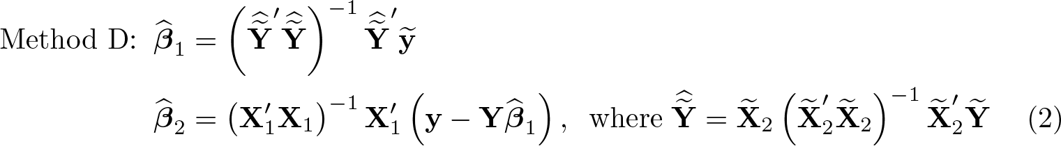
However, this approach reinserts estimates $\widehat{Y}$ based upon nearly collinear regressors Z alongside possibly nearly collinear regressors X ₁, repeating the estimation of a nearly collinear inverse with the addition of new variables, potentially magnifying computation errors. A better approach might be to make use of the partitioned regression given by

$\begin{array}{l}\text{Method}\hspace{0.17em}\text{D}:\hspace{0.17em}{\widehat{\beta }}_1={\left({\widehat{\widetilde{\mathbf{\text{Y}}}}}^{\prime }\widehat{\widetilde{\mathbf{\text{Y}}}}\right)}^{-1}\hspace{0.17em}{\widehat{\widetilde{\mathbf{\text{Y}}}}}^{\prime }\tilde{y}\\ \hspace{0.17em}{\widehat{\beta }}_2={\left({X^{\prime }}_1{X}_1\right)}^{-1}\hspace{0.17em}{X^{\prime }}_1\left(y\hspace{0.17em}-\hspace{0.17em}Y{\widehat{\beta }}_1\right)\text{,}\hspace{0.17em}\text{ where}\hspace{0.17em} \widehat{\tilde{\mathbf{Y}}}={\tilde{X}}_2\hspace{0.17em}{\left({\tilde{X}}_2^{\prime }{\tilde{X}}_2\right)}^{-1}\hspace{0.17em}{\tilde{X}}_2^{\prime }\tilde{Y}\\ \hspace{0.17em}\end{array}$

2

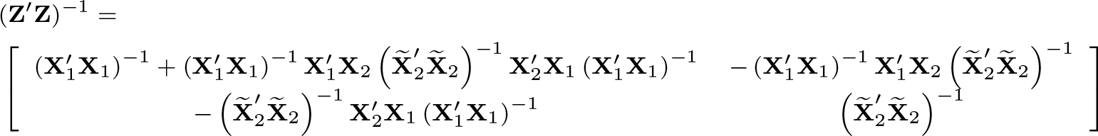
and where ∼ denotes residuals from the projection on X ₁, as in $\tilde{Y}=Y\hspace{0.17em}-\hspace{0.17em}{X}_1{\left({X^{\prime }}_1{X}_1\right)}^{-1}\hspace{0.17em}{X^{\prime }}_1\hspace{0.17em}Y$ . Because

$\begin{array}{l}{\left(Z^{\prime }Z\right)}^{-1}=\\ \hspace{0.17em}\left[\begin{array}{cc}{\left({X^{\prime }}_1{X}_1\right)}^{-1}+{\left({X^{\prime }}_1{X}_1\right)}^{-1}{X^{\prime }}_1{X}_2{\left({\tilde{X}}_2^{\prime }{\tilde{X}}_2\right)}^{-1}{X^{\prime }}_2{X}_1{\left({X^{\prime }}_1{X}_1\right)}^{-1}& -\hspace{0.17em}{\left({X^{\prime }}_1{X}_1\right)}^{-1}{X^{\prime }}_1{X}_2{\left({\tilde{X}}_2^{\prime }{\tilde{X}}_2\right)}^{-1}\\ -{\left({\tilde{X}}_2^{\prime }{\tilde{X}}_2\right)}^{-1}{X^{\prime }}_2{X}_1{\left({X^{\prime }}_1{X}_1\right)}^{-1}& {\left({\tilde{X}}_2^{\prime }{X}_2\right)}^{-1}\end{array}\right]\end{array}$

provides all the inverses used in (2), implementation of method D amounts to calculating the nearly collinear matrix inverse (Z ′ Z) ^{− 1}once and only once.

One may also improve computational accuracy by not actually calculating matrix inverses. Many of the matrix operations in methods A–D above involve calculating x = A ^{− 1} b, where x and b are vectors and A is a symmetric matrix. Rather than calculating the inverse, one can consider this as solving for x in the linear system Ax = b. Solutions of linear systems involve fewer calculations than matrix inversion and hence less opportunity for floating-point errors to cumulate. When A is known to be symmetric positive definite, use of the Cholesky decomposition CC ′ = A further reduces the number of calculations needed (Press et al. 2007). Unfortunately, however, solving x = A ^{− 1} b as the linear system Ax = b for each instance of b implicitly allows the matrix inverse of A to vary across the calculations used in computing the 2SLS coefficients. As shown below, this becomes a consideration when the coefficients are already calculated with a high degree of accuracy using the matrix inverse approach.

Another way to improve computational accuracy is by improving the “conditioning” of matrices. In matrix algebra, the condition number of a positive-definite matrix, the ratio of the largest to smallest eigenvalues, is a measure of the sensitivity of the solution for x in x = A ^{− 1} b to errors in the computation of b (Watkins 2002). ⁴ If we divide the matrix of instruments Z into Z ₁ and Z ₂ (not necessarily corresponding to the included and excluded instruments X ₁ and X ₂), then it is easily shown that the condition number of the matrix Z ′ Z is always worse than that of ${Z^{\prime }}_1\left\{I\hspace{0.17em}-\hspace{0.17em}{Z}_2{\left({Z^{\prime }}_2{Z}_2\right)}^{-1}\hspace{0.17em}{Z^{\prime }}_2\right\}{Z}_1$ , that is, the matrix of residuals of Z ₁ projected on Z ₂. In addition, the dimensionality of the matrix of residuals is smaller, reducing the number of calculations. Consequently, provided ${\left({Z^{\prime }}_2{Z}_2\right)}^{-1}$ can be calculated exactly and the coefficients associated with Z ₂ easily calculated given the coefficient estimates associated with Z ₁, partitioning the regression this way can improve accuracy. These conditions are satisfied when the regression contains a constant term or dummy variables, and I show below that demeaning the remaining variables greatly improves the accuracy of all the methods described above. ⁵ Although the code for Stata’s ivregress (earlier, ivreg) and xtivreg commands is not transparent, because the ado-files call the internal command _regress, as shown below, their sensitivity to near collinearity is on par with that found using method A with demeaned variables and matrix inverses rather than linear solutions.

5 Testing on nearly collinear datasets

To test the relative accuracy of the procedures described above, as well as that of Stata’s built-in IV commands and supplemental community-contributed commands, I draw upon a broad sample of Stata-based 2SLS regressions published in American Economic Association journals examined in Young (2022). The sample covers 967 2SLS specifications in 29 articles ⁶ (including Oreopoulos [2006]) and is restricted to regressions that have only one endogenous variable because specifications with more than that were found to be exceedingly rare. Ninety-one of these specifications have zero or one included instrument other than the constant term. Because the rotation procedure I use below to increase collinearity requires more than one such instrument, these regressions are dropped, leaving 876 2SLS specifications—39 in Oreopoulos and 837 in 28 other articles. As a summary measure of collinearity, I use the maximum partial R ² (net of any absorbed fixed effects) found in the regression of one instrument in Z on the others (hereafter R ^2Max). In the online appendix, I prove that −log(1 − R ^2Max) bounds the lowest log-condition number attainable through diagonal rescaling and find it explains as much of the variation in the sensitivity of 2SLS results shown below as the condition numbers of the matrix of demeaned instruments, although the condition numbers do have the edge in tests of statistical significance.

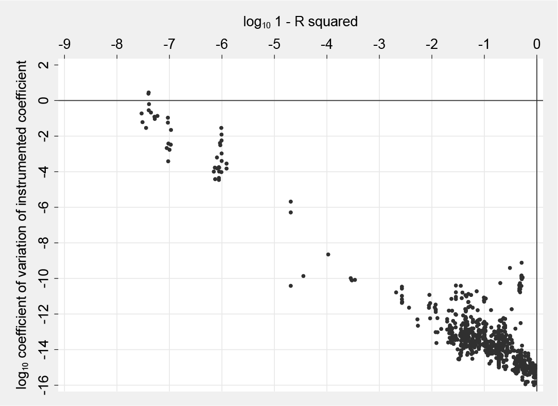
For the sample described above, I randomly permute the order of the included instruments (other than absorbed fixed effects and the constant term) 50 times and calculate the coefficient of variation of the coefficient on the endogenous (instrumented) regressor using Stata’s built-in estimation commands ivregress and xtivreg. ⁷ Figure 1 below graphs the logarithm of these against the logarithm in base 10 (to ease interpretation) of 1 − R ^2Max. As shown, there is a strong relationship between the degree of collinearity and the coefficient of variation, but the sensitivity found in these articles (outside of Oreopoulos [2006] in the upper left corner of the figure), while measurable, is not of substantive concern. To test alternative 2SLS computation procedures, I increase collinearity using a rotation procedure that theoretically, but not computationally, should be econometrically irrelevant.

Figure 1.

Coefficient of variation of instrumented coefficients across 50 permutations of variable order (876 IV regressions in 29 articles—6 coefficients of variation are 0 and not shown in the figure)

For the N × k ₁ − 1 matrix X _{1 ∼ c} of exogenous regressors other than the constant term and absorbed fixed effects, consider the rotation given by $X_{1~c}^{*}=X_{1~c}\left\{U\hspace{0.17em}+\hspace{0.17em}iI\left(k_1\hspace{0.17em}-\hspace{0.17em}1\right)\right\}$ , where U is a k ₁ – 1 × k ₁ − 1 matrix of i.i.d draws from the uniform distribution on (0, 1), I(k ₁ − 1) is the k ₁ − 1 dimensional identity matrix, and i is an integer scalar. $X_{1~c}^{*}$ is often highly collinear because each of the instruments is a linear function of the same k ₁ −1 variables, but $X_{1~c}^{*}$ and X_{1 ∼ c} span exactly the same space. Consequently, because the excluded instruments are not included in X_{1 ∼ c} , the rotation does not compromise the exclusion restriction and identification of the effect of the instrumented variable. After rotating X_{1 ∼ c} to $X_{1~c}^{*}$ in each specification and calculating the new R ^2Max, I then permute the order of the variables in $X_{1~c}^{*}$ 50 times and calculate the coefficient of variation of the estimated coefficients across these permutations. With near-collinear regressors, Stata commands often drop regressors, turning nearly collinear matrices into well-conditioned ones. The scalar i in $X_{1~c}^{*}=X_{1~c}\left\{U\hspace{0.17em}+\hspace{0.17em}iI\left(k_1\hspace{0.17em}-\hspace{0.17em}1\right)\right\}$ avoids this by reducing collinearity among the regressors. For each specification, I calculate $X_{1~c}^{*}$ for each value of i = 1, 2, 3,…, continuing up through the integers until I have 10 instances where, in 50 permutations of variable order, all regressors are retained by the Stata IV commands ivreg and ivregress (or, with fixed effects, xtivreg) and communitycontributed command ivreg2 (xtivreg2). ⁸ Thus, in each instance the variables are collinear but not collinear enough to be flagged and dropped by existing commands.

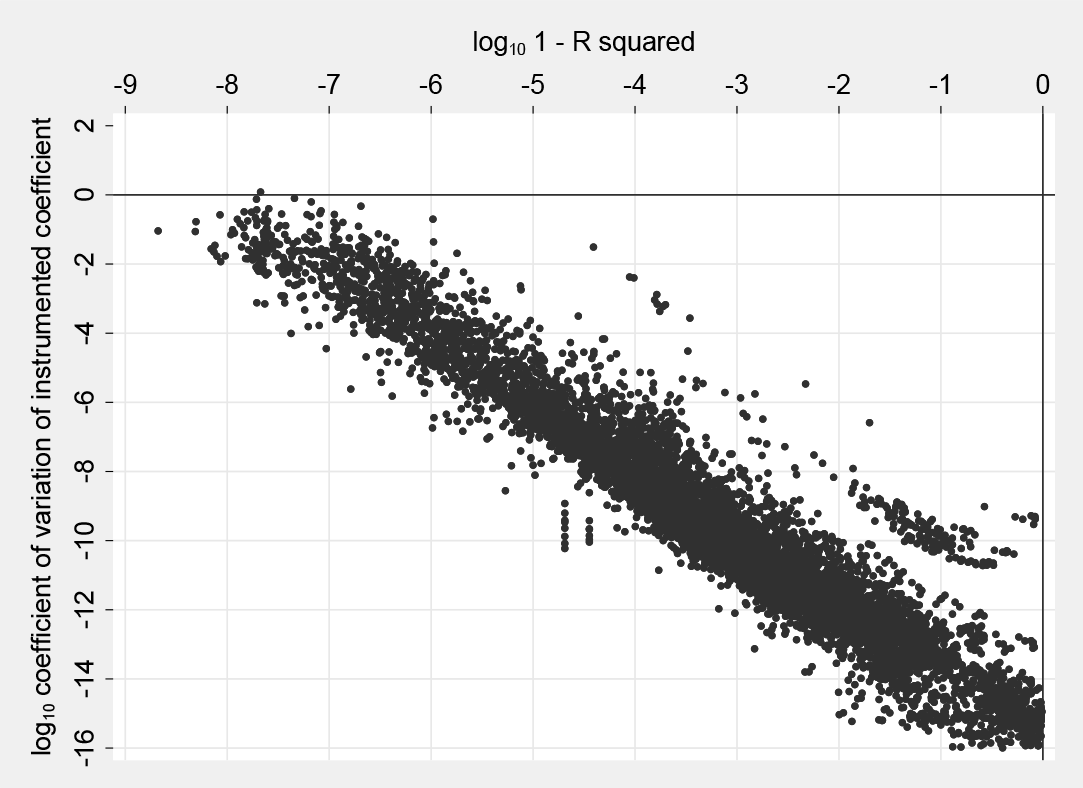
Figure 2 graphs the log₁₀ coefficient of variation using ivregress and xtivreg of the instrumented coefficient estimate across 50 permutations of instrument order against log₁₀(1−R ^2Max) for each of the 10 rotations of the included instruments in the 837 2SLS regressions of the 28 articles (excluding Oreopoulos [2006]) in my sample. As shown, the rotations introduce a range of collinearity, with the highest degree of collinearity often generating a sensitivity similar to that found in Oreopoulos (2006), although there is considerable heterogeneity in the sensitivity of results in different articles to increasing collinearity. Regressions in the online appendix show that the coefficient of variation is increasing in the influence conditioning on the covariates has on the instrumented point estimate (as shown for Oreopoulos [2006] earlier above) but is not significantly related to the strength of the first stage or the number of observations or instruments.

Figure 2.

Coefficient of variation of instrumented coefficients across 50 permutations of variable order (8,370 observations from 10 instrument rotations in 837 regressions in 28 articles—32 coefficients of variation are 0 and not shown in the figure)

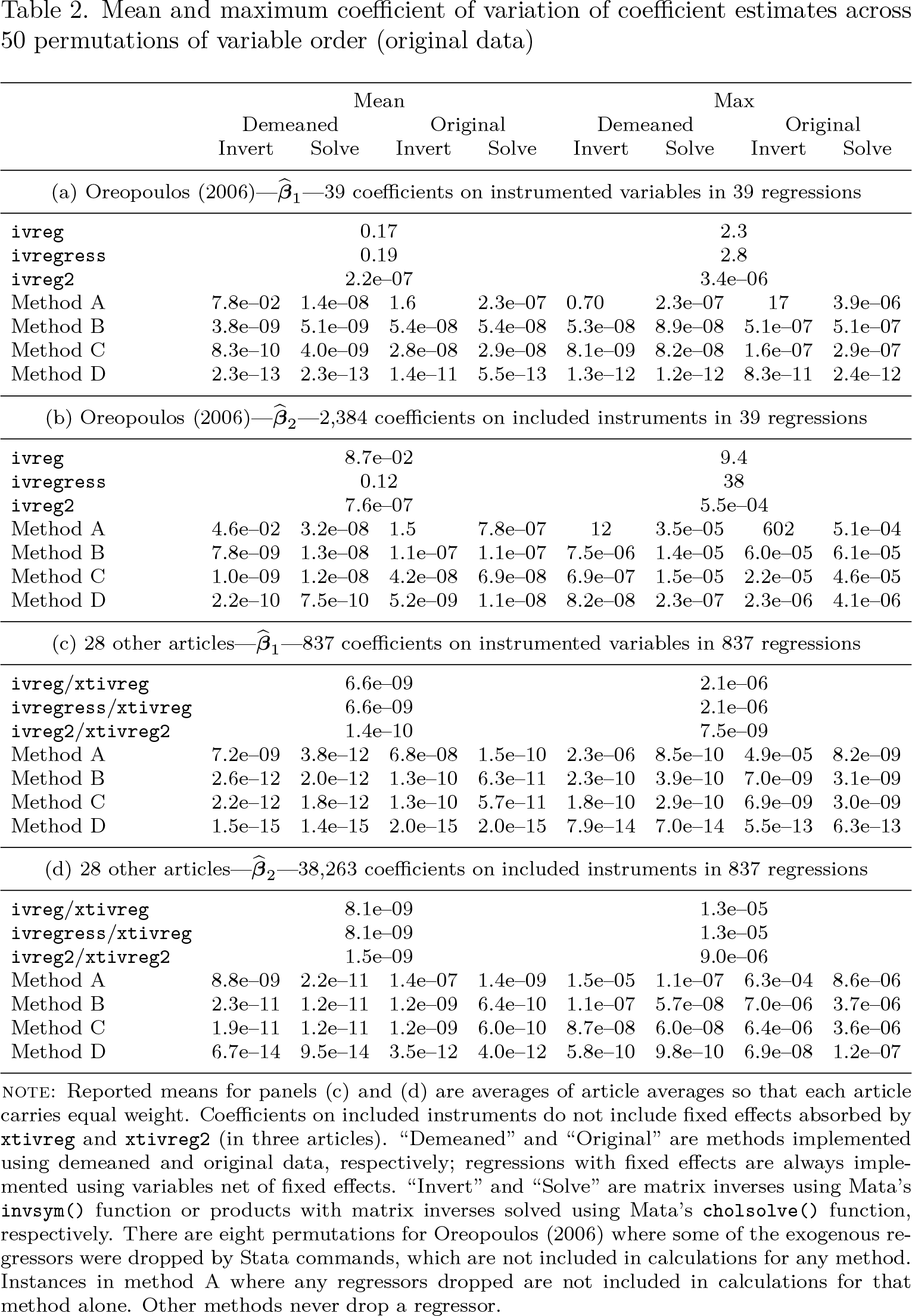
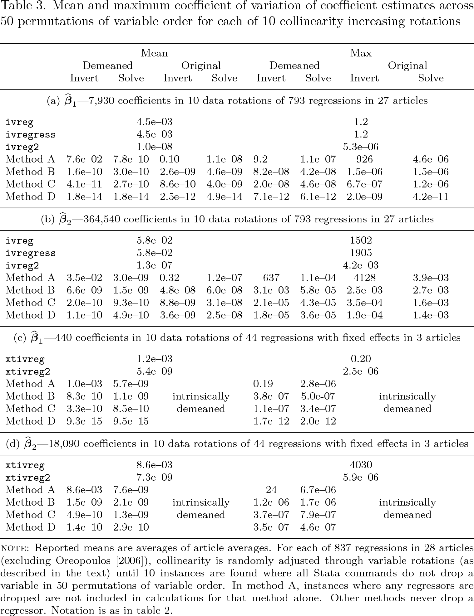
Tables 2 and 3 below compare the accuracy of different 2SLS computational methods, with table 2 focusing on original data and table 3 on the nearly collinear samples created by the rotation procedure described above. Reported are results for Stata’s ivreg, ivregress, and xtivreg commands, the community-contributed commands ivreg2 and xtivreg2, and direct computation using the four methods described above in Stata’s programming language Mata. Results labeled “Demeaned” partition out the effect of the constant term, using the demeaned values of the remaining regressors, while those labeled “Original” use calculations including the constant term in the matrix of regressors. Results labeled “Invert” invert matrices once and use them for all subsequent calculations, while those labeled “Solve” compute each product of a matrix inverse with a vector as a separate Cholesky-based solution of a linear system. Mean and maximum coefficients of variation are reported separately for the coefficients on the instrumented variable $\left({\widehat{\beta }}_1\right)$ and the included instruments $\left({\widehat{\beta }}_2\right)$ . When the data are demeaned, the coefficients on the constant term are recovered using the point estimates for the other effects and their results included in the reported figures. Because the number of regres sions and coefficients varies greatly by article (see Young [2022]), reported multiarticle means here and further below are calculated as the average of article averages so that each article carries equal weight.

Table 2.

Mean and maximum coefficient of variation of coefficient estimates across 50 permutations of variable order (original data)

	Mean				Max
	Demeaned		Original		Demeaned		Original
	Invert	Solve	Invert	Solve	Invert	Solve	Invert	Solve
(a) Oreopoulos (2006)— ${\widehat{\beta }}_1$ —39 coefficients on instrumented variables in 39 regressions
ivreg	0.17				2.3
ivregress	0.19				2.8
ivreg2	2.2e–07				3.4e–06
Method A	7.8e–02	1.4e–08	1.6	2.3e–07	0.70	2.3e–07	17	3.9e–06
Method B	3.8e–09	5.1e–09	5.4e–08	5.4e–08	5.3e–08	8.9e–08	5.1e–07	5.1e–07
Method C	8.3e–10	4.0e–09	2.8e–08	2.9e–08	8.1e–09	8.2e–08	1.6e–07	2.9e–07
Method D	2.3e–13	2.3e–13	1.4e–11	5.5e–13	1.3e–12	1.2e–12	8.3e–11	2.4e–12
(b) Oreopoulos (2006)— ${\widehat{\beta }}_2$ —2,384 coefficients on included instruments in 39 regressions
ivreg	8.7e–02				9.4
ivregress	0.12				38
ivreg2	7.6e–07				5.5e–04
Method A	4.6e–02	3.2e–08	1.5	7.8e–07	12	3.5e–05	602	5.1e–04
Method B	7.8e–09	1.3e–08	1.1e–07	1.1e–07	7.5e–06	1.4e–05	6.0e–05	6.1e–05
Method C	1.0e–09	1.2e–08	4.2e–08	6.9e–08	6.9e–07	1.5e–05	2.2e–05	4.6e–05
Method D	2.2e–10	7.5e–10	5.2e–09	1.1e–08	8.2e–08	2.3e–07	2.3e–06	4.1e–06
(c) 28 other articles— ${\widehat{\beta }}_1$ —837 coefficients on instrumented variables in 837 regressions
ivreg/xtivreg	6.6e–09				2.1e–06
ivregress/xtivreg	6.6e–09				2.1e–06
ivreg2/xtivreg2	1.4e–10				7.5e–09
Method A	7.2e–09	3.8e–12	6.8e–08	1.5e–10	2.3e–06	8.5e–10	4.9e–05	8.2e–09
Method B	2.6e–12	2.0e–12	1.3e–10	6.3e–11	2.3e–10	3.9e–10	7.0e–09	3.1e–09
Method C	2.2e–12	1.8e–12	1.3e–10	5.7e–11	1.8e–10	2.9e–10	6.9e–09	3.0e–09
Method D	1.5e–15	1.4e–15	2.0e–15	2.0e–15	7.9e–14	7.0e–14	5.5e–13	6.3e–13
(d) 28 other articles— ${\widehat{\beta }}_2$ —38,263 coefficients on included instruments in 837 regressions
ivreg/xtivreg	8.1e–09				1.3e–05
ivregress/xtivreg	8.1e–09				1.3e–05
ivreg2/xtivreg2	1.5e–09				9.0e–06
Method A	8.8e–09	2.2e–11	1.4e–07	1.4e–09	1.5e–05	1.1e–07	6.3e–04	8.6e–06
Method B	2.3e–11	1.2e–11	1.2e–09	6.4e–10	1.1e–07	5.7e–08	7.0e–06	3.7e–06
Method C	1.9e–11	1.2e–11	1.2e–09	6.0e–10	8.7e–08	6.0e–08	6.4e–06	3.6e–06
Method D	6.7e–14	9.5e–14	3.5e–12	4.0e–12	5.8e–10	9.8e–10	6.9e–08	1.2e–07

NOTE: Reported means for panels (c) and (d) are averages of article averages so that each article carries equal weight. Coefficients on included instruments do not include fixed effects absorbed by xtivreg and xtivreg2 (in three articles). “Demeaned” and “Original” are methods implemented using demeaned and original data, respectively; regressions with fixed effects are always implemented using variables net of fixed effects. “Invert” and “Solve” are matrix inverses using Mata’s invsym() function or products with matrix inverses solved using Mata’s cholsolve() function, respectively. There are eight permutations for Oreopoulos (2006) where some of the exogenous regressors were dropped by Stata commands, which are not included in calculations for any method. Instances in method A where any regressors dropped are not included in calculations for that method alone. Other methods never drop a regressor.

Table 3.

Mean and maximum coefficient of variation of coefficient estimates across 50 permutations of variable order for each of 10 collinearity increasing rotations

		Mean					Max
	Demeaned		Original		Demeaned		Original
	Invert	Solve	Invert	Solve	Invert	Solve	Invert	Solve
(a) ${\widehat{\beta }}_1$ —7,930 coefficients in 10 data rotations of 793 regressions in 27 articles
ivreg	4.5e–03 4.5e–03 1.0e–08				1.2 1.2 5.3e–06
ivregress
ivreg2
Method A	7.6e–02	7.8e–10	0.10	1.1e–08	9.2	1.1e–07	926	4.6e–06
Method B	1.6e–10	3.0e–10	2.6e–09	4.6e–09	8.2e–08	4.2e–08	1.5e–06	1.5e–06
Method C	4.1e–11	2.7e–10	8.6e–10	4.0e–09	2.0e–08	4.6e–08	6.7e–07	1.2e–06
Method D	1.8e–14	1.8e–14	2.5e–12	4.9e–14	7.1e–12	6.1e–12	2.0e–09	4.2e–11
(b) ${\widehat{\beta }}_2$ —364,540 coefficients in 10 data rotations of 793 regressions in 27 articles
ivreg	5.8e–02 5.8e–02 1.3e–07				1502 1905 4.2e–03
ivregress
ivreg2
Method A	3.5e–02	3.0e–09	0.32	1.2e–07	637	1.1e–04	4128	3.9e–03
Method B	6.6e–09	1.5e–09	4.8e–08	6.0e–08	3.1e–03	5.8e–05	2.5e–03	2.7e–03
Method C	2.0e–10	9.3e–10	8.8e–09	3.1e–08	2.1e–05	4.3e–05	3.5e–04	1.6e–03
Method D	1.1e–10	4.9e–10	3.6e–09	2.5e–08	1.8e–05	3.6e–05	1.9e–04	1.4e–03
(c) ${\widehat{\beta }}_1$ —440 coefficients in 10 data rotations of 44 regressions with fixed effects in 3 articles
xtivreg	1.2e–03 5.4e–09				0.20 2.5e–06
xtivreg2
Method A	1.0e–03	5.7e–09			0.19	2.8e–06
Method B	8.3e–10	1.1e–09	intrinsically		3.8e–07	5.0e-07	intrinsically
Method C	3.3e–10	8.5e–10	demeaned		1.1e–07	3.4e–07	demeaned
Method D	9.3e–15	9.5e–15			1.7e–12	2.0e–12
(d) ${\widehat{\beta }}_2$ —18,090 coefficients in 10 data rotations of 44 regressions with fixed effects in 3 articles
xtivreg	8.6e–03 7.3e–09				4030 5.9e–06
xtivreg2
Method A	8.6e–03	7.6e–09			24	6.7e–06
Method B	1.5e–09	2.1e–09	intrinsically		1.2e–06	1.7e–06	intrinsically
Method C	4.9e–10	1.3e–09	demeaned		3.7e–07	7.9e–07	demeaned
Method D	1.4e–10	2.9e–10			3.5e–07	4.6e–07

NOTE: Reported means are averages of article averages. For each of 837 regressions in 28 articles (excluding Oreopoulos [2006]), collinearity is randomly adjusted through variable rotations (as described in the text) until 10 instances are found where all Stata commands do not drop a variable in 50 permutations of variable order. In method A, instances where any regressors are dropped are not included in calculations for that method alone. Other methods never drop a regressor. Notation is as in table 2.

I begin by noting that Stata’s official commands ivreg, ivregress, and xtivreg are among the worst performing. True to Stata’s documentation, these commands appear to use method A, producing results that are better than the rock-bottom performance using method A with original data but without achieving the improvements that come from demeaning, let alone the use of solvers rather than matrix inverses. ivregress produces results similar to the program it superseded, ivreg, but in Oreopoulos’s (2006) data on average and in worst-case situations (maximums), the results are worse. ⁹ The community-contributed commands ivreg2 and xtivreg2 are orders of magnitude less sensitive than Stata’s built-in commands, producing results that are consistently very close to those found with method A and the use of linear solutions but without (in the case of ivreg2) attaining the additional improvement found by demeaning. ¹⁰ Turning to the rest of the table, we see that calculations become systematically less sensitive to permutations of variable order as one moves from method A to B to C to D and that demeaning and use of linear solutions confer large advantages, especially when using less accurate techniques such as method A. However, once method D is used, linear solvers actually appear to worsen accuracy because, as noted above, they implicitly allow the inverse of a given matrix to vary when solving different linear systems. Method D with demeaned variables is orders of magnitude less sensitive to collinearity than the community-contributed commands ivreg2 and xtivreg2, although the latter are unlikely to display discernible sensitivity to variable order in the environments encountered in practical work (including Oreopoulos [2006]).

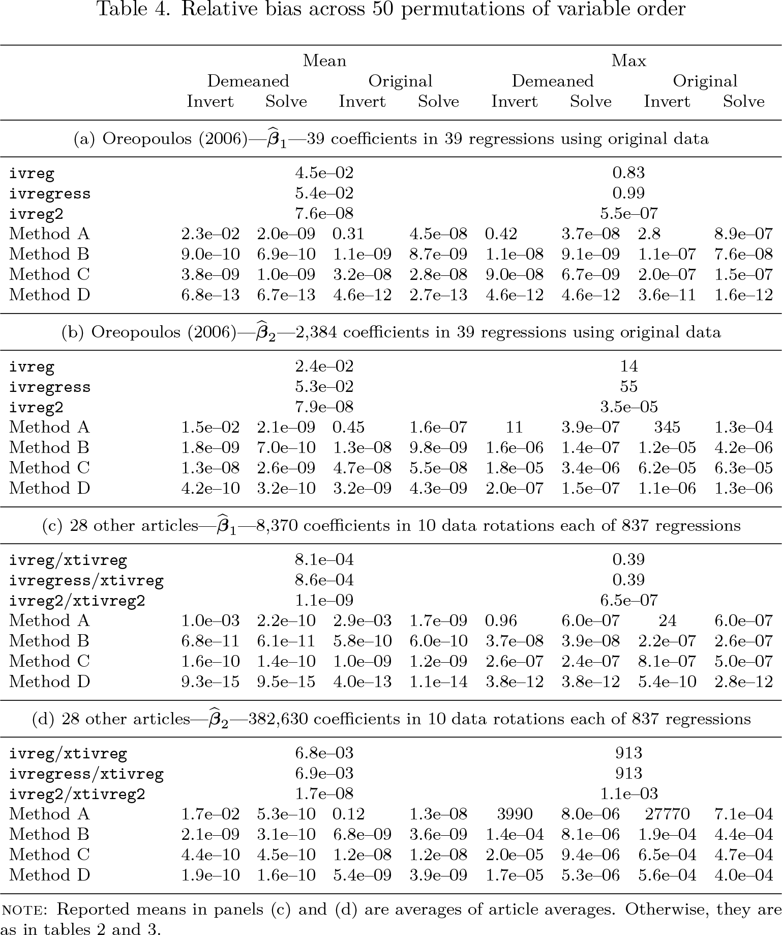
Lack of sensitivity to variable order is not equivalent to accuracy, because it is possible for a procedure to consistently provide incorrect estimates. To establish benchmark “true” values for the estimating equations in my sample, I calculate point estimates at 100-digit precision using the Advanpix Multiprecision Computing Toolbox for MATLAB. When rounded to double precision, these estimates are identical across methods A through D implemented with and without demeaning or linear solutions for all 50 reorderings of Oreopoulos’s regressors used in table 2; that is, they display zero sensitivity to variable order. Using the 100-digit precision rounded to double precision values produced by the Advanpix Toolbox as the benchmark, table 4 below reports the average relative absolute bias of the mean Stata coefficient estimates across 50 permutations of variable order. That is, with ${\widehat{\beta }}_i$ (100) representing the 100-digit precision estimate rounded to double precision and ${\overline{\widehat{\beta }}}_i$ (method) representing the mean double precision point estimate across 50 random variable orders of methods A–D and the Stata commands in the tables, table 4 reports the average and maximum value of $|\{{\overline{\widehat{\beta }}}_i(\text{ method })\hspace{0.17em}-\hspace{0.17em}{\widehat{\beta }}_i(100)\}/{\widehat{\beta }}_i(100)|$ for the original data of Oreopoulos (2006) and the 10 collinearity-increasing rotations of the data of the other 28 articles. The patterns follow the results of the previous tables, with Stata’s built-in commands recording maximum relative bias as high as 0.99 on the instrumented coefficient and 913 on included instruments, ivreg2 and xtivreg2 lowering worst-case outcomes to acceptable levels, and methods B through D successively lowering relative bias orders of magnitude further.

Table 4.

Relative bias across 50 permutations of variable order

	Mean				Max
	Demeaned		Original		Demeaned		Original
	Invert	Solve	Invert	Solve	Invert	Solve	Invert	Solve
(a) Oreopoulos (2006)— ${\widehat{\beta }}_1$ —39 coefficients in 39 regressions using original data
ivreg	4.5e–02				0.83
ivregress	5.4e–02				0.99
ivreg2	7.6e–08				5.5e–07
Method A	2.3e–02	2.0e–09	0.31	4.5e–08	0.42	3.7e–08	2.8	8.9e–07
Method B	9.0e–10	6.9e–10	1.1e–09	8.7e–09	1.1e–08	9.1e–09	1.1e–07	7.6e–08
Method C	3.8e–09	1.0e–09	3.2e–08	2.8e–08	9.0e–08	6.7e–09	2.0e–07	1.5e–07
Method D	6.8e–13	6.7e–13	4.6e–12	2.7e–13	4.6e–12	4.6e–12	3.6e–11	1.6e–12
(b) Oreopoulos (2006)— ${\widehat{\beta }}_2$ —2,384 coefficients in 39 regressions using original data
ivreg	2.4e–02 5.3e–02 7.9e–08				14 55 3.5e–05
ivregress
ivreg2
Method A	1.5e–02	2.1e–09	0.45	1.6e–07	11	3.9e–07	345	1.3e–04
Method B	1.8e–09	7.0e–10	1.3e–08	9.8e–09	1.6e–06	1.4e–07	1.2e–05	4.2e–06
Method C	1.3e–08	2.6e–09	4.7e–08	5.5e–08	1.8e–05	3.4e–06	6.2e–05	6.3e–05
Method D	4.2e–10	3.2e–10	3.2e–09	4.3e–09	2.0e–07	1.5e–07	1.1e–06	1.3e–06
(c) 28 other articles— ${\widehat{\beta }}_1$ —8,370 coefficients in 10 data rotations each of 837 regressions
ivreg/xtivreg	8.1e–04				0.39
ivregress/xtivreg	8.6e–04				0.39
ivreg2/xtivreg2	1.1e–09				6.5e–07
Method A	1.0e–03	2.2e–10	2.9e–03	1.7e–09	0.96	6.0e–07	24	6.0e–07
Method B	6.8e–11	6.1e–11	5.8e–10	6.0e–10	3.7e–08	3.9e–08	2.2e–07	2.6e–07
Method C	1.6e–10	1.4e–10	1.0e–09	1.2e–09	2.6e–07	2.4e–07	8.1e–07	5.0e–07
Method D	9.3e–15	9.5e–15	4.0e–13	1.1e–14	3.8e–12	3.8e–12	5.4e–10	2.8e–12
(d) 28 other articles— ${\widehat{\beta }}_2$ —382,630 coefficients in 10 data rotations each of 837 regressions
ivreg/xtivreg	6.8e–03				913
ivregress/xtivreg	6.9e–03				913
ivreg2/xtivreg2	1.7e–08				1.1e–03
Method A	1.7e–02	5.3e–10	0.12	1.3e–08	3990	8.0e–06	27770	7.1e–04
Method B	2.1e–09	3.1e–10	6.8e–09	3.6e–09	1.4e–04	8.1e–06	1.9e–04	4.4e–04
Method C	4.4e–10	4.5e–10	1.2e–08	1.2e–08	2.0e–05	9.4e–06	6.5e–04	4.7e–04
Method D	1.9e–10	1.6e–10	5.4e–09	3.9e–09	1.7e–05	5.3e–06	5.6e–04	4.0e–04

NOTE: Reported means in panels (c) and (d) are averages of article averages. Otherwise, they are as in tables 2 and 3.

6 The pariv command

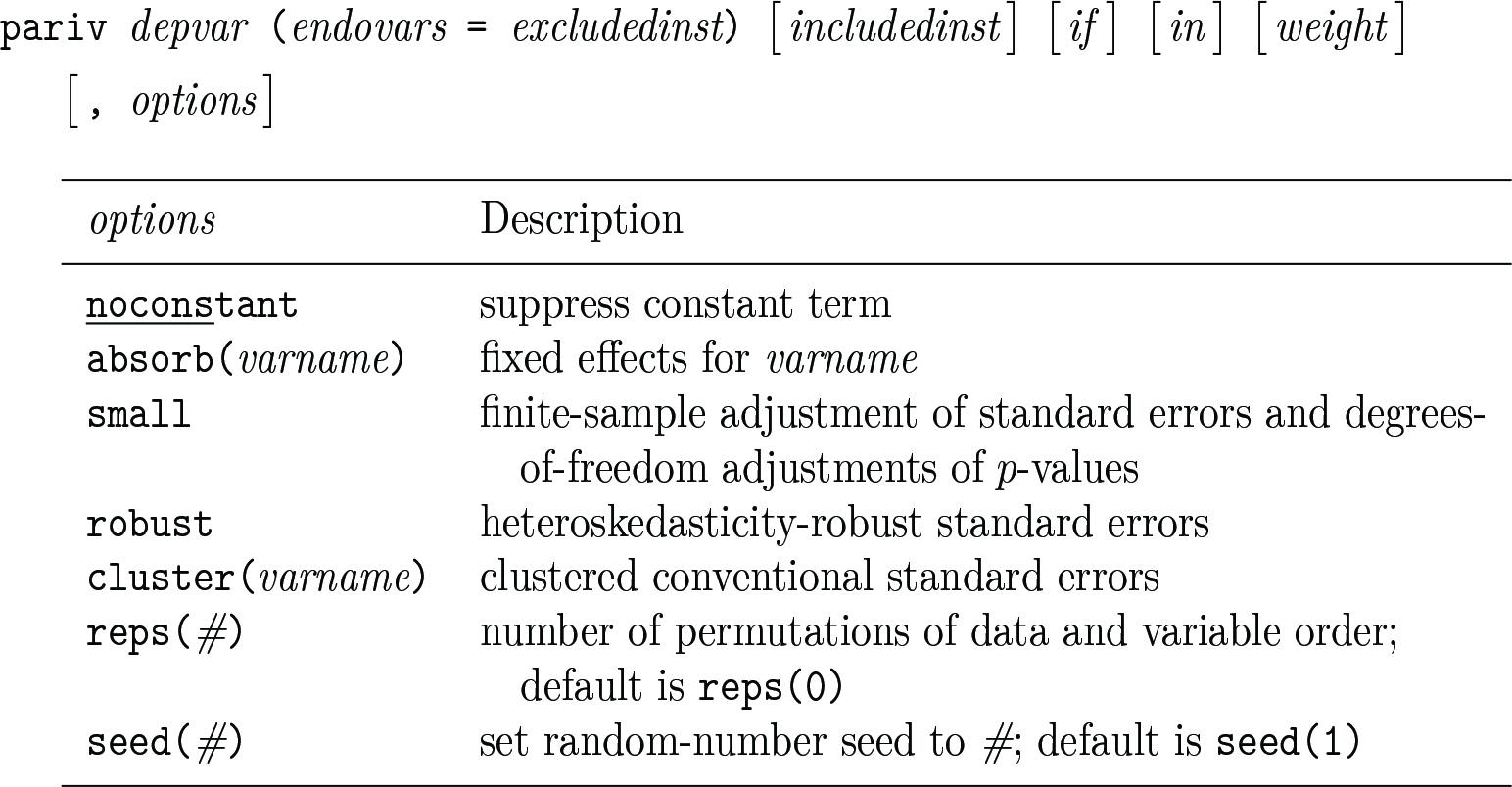
For Stata users concerned about near collinearity in their IV regression, pariv implements partitioned 2SLS (method D) using matrix inverses on demeaned data and, if desired, calculates the sensitivity of reported estimates to random permutations of data and variable order. The syntax and options are

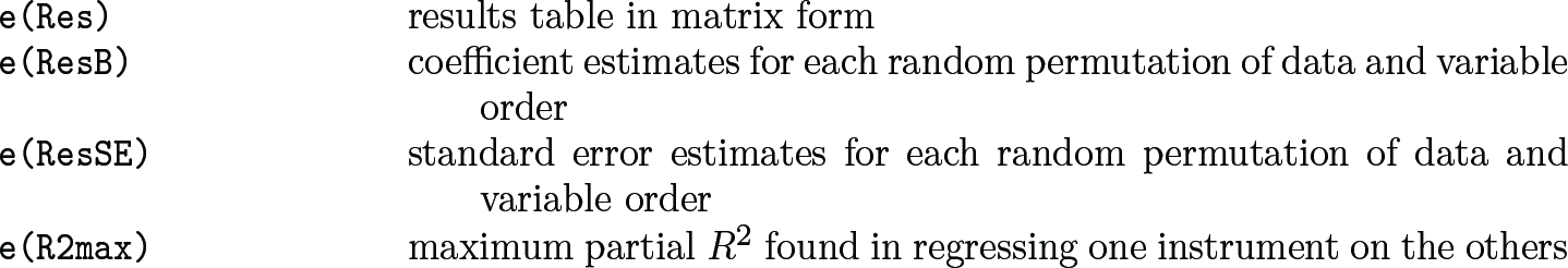
pariv fits the partitioned 2SLS regression of depvar on endovars, includedinst, and (if specified) fixed effects for varname using excludedinst (as well as includedinst and any fixed effects) as instruments for endovars. To check that reported results are not substantively sensitive to econometrically irrelevant procedures, the user may call for reps() simultaneous permutations of data and variable order. pariv will then report the minimum to maximum range of the coefficient and standard error estimates of the partitioned regression across those permutations. pariv stores the following results in e():

Matrices

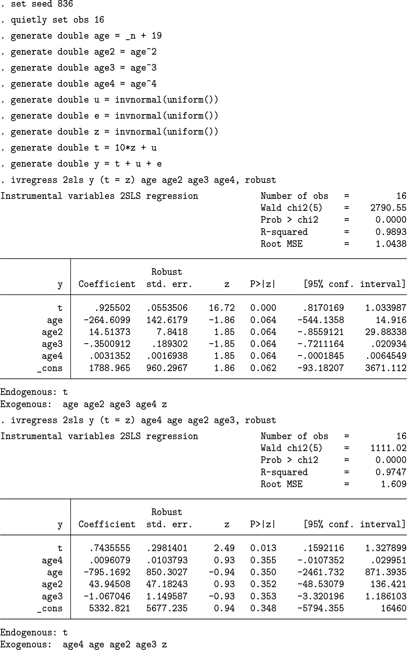
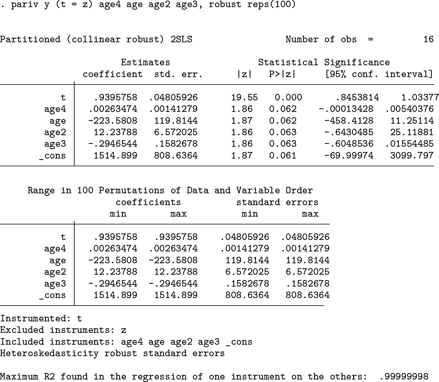
The following code provides an illustrative example in which ivregress’s coefficient and standard error estimates depend heavily upon the order of the variables but the collinear robust estimates produced by pariv do not (results for ivregress may vary with the processor used):

The minimum and maximum coefficient and standard error estimates are identical up to seven significant digits, and the user can be confident that the reported results are not substantively sensitive to econometrically irrelevant procedures.

7 Conclusion

The preceding results suggest that Stata users should avoid Stata’s official ivregress and xtivreg commands and instead use the computationally more accurate community-contributed commands ivreg2 and xtivreg2. At levels of near collinearity that do not induce variable drops in either the original data of Oreopoulos (2006) or collinearity-increasing rotations of the data of 28 other articles, these commands provide results that are accurate and totally insensitive to econometrically irrelevant procedures within the range of typically reported significant figures. For users who might nevertheless harbor concerns or curiosity, this article provides pariv, which checks the sensitivity of the results and gauges (in the maximum R ² of one variable projected on the others) the degree of near collinearity of the data. pariv is designed to be a confidence-boosting check of computational accuracy and otherwise lacks the broad functionality found in ivreg2 and xtivreg2.

Stata’s computational methods are surprising, not least because Gould (2018), who is Stata’s founding programmer, emphasizes the importance of computational accuracy and use of techniques such as demeaning and linear solutions that are clearly not consistently applied in Stata’s IV code. Additionally, the unnecessary and almost always incorrect assumption that a calculated matrix inverse times the matrix itself is exactly equal to the identity matrix (method A above) appears to be a defining feature of all Stata IV code, including community-contributed commands. As Gould emphasizes, it is incumbent upon programmers to maximize computational accuracy, saving users the need to concern themselves with econometrically irrelevant issues. To this end, the tables above provide systematic evidence of the benefits of demeaning, linear solutions, and partitioning of regressions in a broad practical sample.

8 Programs and supplemental material

Supplemental Material, sj-zip-1-stj-10.1177_1536867X241233668 - Nearly collinear robust procedures for 2SLS estimation

Supplemental Material, sj-zip-1-stj-10.1177_1536867X241233668 for Nearly collinear robust procedures for 2SLS estimation by Alwyn Young in The Stata Journal

References

1.
BaumC. F.SchafferM. E.StillmanS.. 2002. ivreg2: Stata module for extended instrumental variables/2SLS and GMM estimation. Statistical Software Components S425401, Department of Economics, Boston College. https://ideas.repec.org/c/boc/bocode/s425401.html.
OreopoulosP.2006. Estimating average and local average treatment effects of education when compulsory schooling laws really matter. American Economic Review96: 152–175. https://doi.org/10.1257/000282806776157641.
6.
PressW. H.TeukolskyS. A.VetterlingW. T.FlanneryB. P.. 2007. Numerical Recipes: The Art of Scientific Computing. 3rd ed. Cambridge: Cambridge University Press.
7.
SchafferM. E. 2005. xtivreg2: Stata module to perform extended IV/2SLS, GMM and AC/HAC, LIML, and k-class regression for panel-data models. Statistical Software Components S456501, Department of Economics, Boston College. https://ideas.repec.org/c/boc/bocode/s456501.html.
8.
SkeelR. D.1979. Scaling for numerical stability in Gaussian elimination. Journal of the Association for Computing Machinery26: 494–526. https://doi.org/10.1145/322139.322148.
9.
StephensM.Jr.YangD.-Y.. 2014. Compulsory education and the benefits of schooling. American Economic Review104: 1777–1792. https://doi.org/10.1257/aer.104.6.1777.
10.
van der SluisA.1969. Condition numbers and equilibration of matrices. Numerische Mathematik14: 14–23. https://doi.org/10.1007/BF02165096.
11.
WatkinsD. S.2002. Fundamentals of Matrix Computations. 2nd ed. New York: Wiley.
Please find the following supplemental material available below.
For Open Access articles published under a Creative Commons License, all supplemental material carries the same license as the article it is associated with.
For non-Open Access articles published, all supplemental material carries a non-exclusive license, and permission requests for re-use of supplemental material or any part of supplemental material shall be sent directly to the copyright owner as specified in the copyright notice associated with the article.