Sage Journals: Discover world-class research

Abstract

We develop a command, weaktsiv, for two-sample instrumentalvariables regression models with one endogenous regressor and potentially weak instruments. weaktsiv includes the classic two-sample two-stage least-squares estimator whose inference is valid only under the assumption of strong instruments. It also includes statistical tests and confidence sets with correct size and coverage probabilities even when the instruments are weak.

Keywords

st0568 weaktsiv two-sample two-stage least squares weak IV inference

1 Introduction

Conventional instrumental-variables (IV) regression requires that the dependent variable, the endogenous regressor, and the instruments come from the same dataset. But in many cases, researchers can observe only the dependent variable and endogenous regressor in two separate data samples (see Björklund and J¨antti [1997], Miguel [2005], Feldman [2010], Brunner, Cho, and Reback [2012], Siminski [2013], Olivetti and Paserman [2015], among many others). Angrist and Krueger (1992, 1995) propose two estimation strategies—two-sample IV and two-sample two-stage least-squares (TS2SLS)—for such two-sample IV regression models. Under the assumption of strong instruments, both two-sample IV and TS2SLS estimators are consistent. Inoue and Solon (2010) provide valid inference formulas for both estimators under the assumption of strong instruments and show that TS2SLS is more efficient. However, when the first stage is weak, neither estimation strategy is valid following arguments similar to the famous Bound, Jaeger, and Baker (1995) critiques in the classic (one-sample) two-stage IV literature.

In a recent study, Choi, Gu, and Shen (2018) develop weak-instrument robust inference for the two-sample IV regression model with one single endogenous regressor. In this article, we develop a command companion, weaktsiv, to this newly proposed inference method. Specifically, the new method extends the classic Anderson–Rubin (see Dufour [1997], Staiger and Stock [1997], Dufour and Jasiak [2001]), Kleibergen (K) (see Kleibergen [2002]), and conditional likelihood-ratio (see Moreira [2003, 2009], Andrews, Moreira, and Stock [2006, 2008]) tests and confidence sets to the two-sample setting. weaktsiv also reports for completeness the classic TS2SLS estimates and associated standard errors. Both cases of homoskedasticity and heteroskedasticity are considered in the proposed command.

Section 2 provides background on the two-sample IV regression model. Section 3 discusses the weak-instrument robust inference methods developed in Choi, Gu, and Shen (2018). Section 4 introduces the new command, weaktsiv. Section 4 gives examples.

2 Model and background

Let subscript j, j = 1, 2, denote random variables in the first or second dataset with sample size n_j . Assume that n ₁ /n ₂ → τ for some fixed τ > 0. In this article, we consider the following two-sample IV regression model with independent and identically distributed data and a single endogenous regressor,

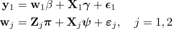
\begin{array}{l} y_{1} = w_{1} β + X_{1} γ + \in_{1} \\ w_{j} = Z_{j} π + X_{j} ψ + ε_{j}, j = 1, 2 \end{array}

where y ₁, w ₁, ∊ ₁, and ε ₁ are n ₁ × 1; w ₂ and ε ₂ are n ₂ × 1; Z _j is n_j × k for j = 1, 2; and X _j is n_j × p for j = 1, 2. All variables in the above model are observed except for w ₁. Researchers are primarily interested in the parameter β in the outcome equation.

TS2SLS follows the idea of classic two-stage least-squares estimation by regressing the outcome variable y ₁ on a predicted endogenous regressor, $\hat{w}$ . Let ${\hat{w}}_{1} = Z_{1} \hat{π} + X_{1} \hat{ψ}$ . Unlike classic two-stage least squares, $\hat{π}$ and $\hat{ψ}$ in TS2SLS are estimated using information from the second data sample because w ₁ is not observed. Specifically, the TS2SLS estimator for β is defined as

{\hat{β}}_{TS2SLS} = ({({\hat{w}}^{'}_{1} M_{X_{1}} {\hat{w}}_{1})}^{- 1} {\hat{w}}^{'}_{1} M_{X_{1}} y_{1})

where ${\hat{w}}_{1} = Z_{1} {({Z^{'}}_{2} M_{X}_{_{2}} Z_{2})}^{- 1} {Z^{'}}_{2} M_{X}_{_{2}} w_{2} + X_{1} {({X^{'}}_{2} M_{Z}_{_{2}} X_{2})}^{- 1} {X^{'}}_{2} M_{Z}_{_{2}} w_{2} .$ For any matrix X, P _X is used to denote X(X′X)⁻¹ X′ and M _X = I − P _X .

Under the assumption that the first-stage correlation between the endogenous regressor and instruments is strong, the TS2SLS estimator is consistent and asymptotically normal. Inoue and Solon (2010) provide inference for TS2SLS under the additional assumptions of homoskedasticity and equal moments of [Z _j X _j ] across the two samples with j = 1, 2. In our model with one endogenous regressor, the Inoue and Solon (2010) formula inflates the second-stage standard errors (that is, standard errors from regressing y ₁ on ${\hat{W}}_{1}$ and X ₁) by a factor of ${1 + (n_{1} / n_{2}) {\hat{β}}_{TS2SLS}^{2} {({\hat{σ}}_{ε 2} / {\hat{σ}}_{u 1})}^{2}}^{\frac{1}{2}},$ where ${\hat{σ}}_{u_{1}}^{2} = {y^{'}}_{1} M_{[Z_{1} : X_{1}]} y_{1} / (n_{1} - k - p)$ and ${\hat{σ}}_{ε_{2}}^{2} = {w^{'}}_{2} M_{[Z_{2} : X_{2}]} w_{2} / (n_{2} - k - p) .$

The additional assumptions on homoskedasticity and equal moments required in Inoue and Solon (2010) could be restrictive in applications. Pacini and Windmeijer (2016) provide TS2SLS inference that is robust to heteroskedasticity and unequal moments of excluded instruments and exogenous regressors, although their results are still not robust to weak instruments. In general, TS2SLS is valid only when the first-stage correlation between instruments and the endogenous regressor is strong.

Table 1 illustrates limitations of the TS2SLS strategy. The data-generating process (DGP) is taken from Choi, Gu, and Shen (2018), where $Z_{1 i} \sim N (0, I_{k}), (\in_{1 i}, e_{1 i}) \sim N (0, I_{2}), \in_{1 i} = 0.1 ε_{1 i} + \sqrt{1 - 0. 1^{2}} e_{1 i}, y_{1 i} = w_{1 i} β + \in_{1 i}, w_{1 i} = Z_{1 i} π + ε_{1 i}, Z_{2 i} \sim N (0, I_{k}), ε_{2 i} \sim N (0, 1),$ and w _2i = Z _2iπ + ε _2i. The sample sizes are n ₁ = 5000 and n ₂ = 1000. The number of instruments is set to 1, 5, or 10. The first-stage coefficient vector π is set to $\sqrt{λ / (n_{2} k)} \times ι,$ where ι is a vector of k ones and λ/k is the concentration parameter capturing the strength of instruments. λ/k is set to 1, 4, or 16.

Table 1 reports the coverage rate of the 95% Inoue and Solon (2010) confidence interval (CI) among 5,000 simulation repetitions as well as the bias and root mean squared error of the TS2SLS estimator. The simulation results show that TS2SLS produces large biases and unreliable CI when the instruments are weak. The 95% CI could have coverage rate as low as 13.7% when there are many weak instruments (k = 10, λ/k = 1). The bias is generally negative when β = 2 and positive when β = −2 because TS2SLS suffers from a classic attenuation bias. The attenuation bias is also inversely proportional to the strength of instruments. See Choi, Gu, and Shen (2018) for more details.

Table 1.

Properties of TS2SLS under weak instruments

Coverage of 95% CI			Bias of estimator			Root mean squared error of estimators
λ/k	1	4	16	1	4	16	1	4	16
(a): β = −2 k = 1	0.767	0.833	0.806	−4.442	0.297	−0.160	180.971	31.051	0.834
k = 5	0.358	0.610	0.715	0.889	0.288	0.076	1.058	0.508	0.249
k = 10	0.137	0.453	0.662	0.955	0.348	0.092	1.018	0.443	0.190
(b): β = 0 k = 1	0.990	0.974	0.956	−0.427	−0.036	−0.001	37.121	3.567	0.128
k = 5	0.961	0.954	0.947	0.002	0.002	0.001	0.168	0.097	0.050
k = 10	0.961	0.950	0.949	0.004	0.001	−0.000	0.109	0.067	0.035
(c): β = 2 k = 1	0.788	0.840	0.819	3.588	−0.370	0.159	160.209	30.845	0.832
k = 5	0.389	0.628	0.735	−0.885	−0.284	−0.074	1.065	0.517	0.251
k = 10	0.165	0.473	0.685	−0.947	−0.346	−0.093	1.018	0.443	0.193

Note: Sample sizes are n₁ = 5000 and n₂ = 1000. Results are based on 5,000 simulation repetitions. The coverage results of the 95% Inoue and Solon (2010) CIs are also reported in Choi, Gu, and Shen (2018).

3 Weak-instrument robust methods

In the following, we introduce the weak-instrument robust inference method discussed in Choi, Gu, and Shen (2018). There are two versions of the method. A benchmark strategy uses the same set of assumptions as Angrist and Krueger (1992, 1995) and Inoue and Solon (2010), except for allowing for potentially weak instruments. The benchmark strategy requires both homoskedasticity and equal moments of excluded instruments and exogenous regressors across the two data samples. In contrast, a fully robust strategy is also considered that makes the two-sample IV inference robust to weak instruments as well as heteroskedasticity and unequal moments. In empirical applications, researchers might want to adopt the fully robust method for its generality and the benchmark method for a direct comparison with the classic Inoue and Solon (2010) results. Starting from this section, we follow the weak inference literature and assume, without loss of generality, that ${Z^{'}}_{j} X_{j} = 0$ for both j = 1, 2. The orthogonality assumption is without loss of generality because one can always define new excluded instruments as residuals from the regression of original instruments on exogenous regressors.

Consider the weak IV asymptotic where the first-stage parameter π is a local sequence converging to zero:

π = C / \sqrt{n_{1}} for some nonstochastic k -vector C

Under this asymptotic, the TS2SLS estimator is no longer consistent. In practice, researchers will consider adopting weak-instrument robust inference methods when the instruments are expected to have weak correlations with the endogenous regressor or when the sample size is small.

3.1 Benchmark weak-instrument robust tests and confidence sets

Let $Y_{1} = [y_{1} {\hat{w}}_{1}], a = {[\begin{matrix} β & 1 \end{matrix}]}^{'}, η = [\begin{matrix} γ & ψ \end{matrix}],$ and V ₁ = [u ₁ v ₁], where γ = γ1 + ψβ, u ₁ = ∊ ₁ + βε₁, and $v_{1} = Z_{1} (\hat{π} - π) + X_{1} (\hat{ψ} - ψ)$ . The simultaneous equation model described in the last section could be rewritten as

Y_{1} = Z_{1} π a' + X_{1} η + V_{1}

In this section, we follow Inoue and Solon (2010) and assume homoskedasticity and equal moments of [Z _j X _j ] for j = 1, 2. Let $σ_{u 1}^{2} = E (u_{1 i}^{2} | Z_{1 i}, X_{1 i}), σ_{ε_{2}}^{2} = E (ε_{2 i}^{2} | Z_{2 i}, X_{2 i})$ and Σ _ZZ be the probability limit of both ${Z^{'}}_{1} Z_{1} / n_{1} and {Z^{'}}_{2} Z_{2} / n_{2} .$

Consider the two-sided null hypothesis H ₀ : β = β ₀ with some predetermined significance level α. Let b ₀ = [1 − β ₀]′, a ₀ = [β ₀ 1]′. Define statistics

\begin{array}{l} {\hat{S}}_{n} = {({z^{'}}_{1} z_{1})}^{- 1 / 2} {Z^{'}}_{1} Y_{1} b_{0} / {({b^{'}}_{0} \hat{Ω} b_{0})}^{1 / 2} \\ {\hat{T}}_{n} = {({z^{'}}_{1} z_{1})}^{- 1 / 2} {Z^{'}}_{1} Y_{1} {\hat{Ω}}^{- 1} a_{0} / {({a^{'}}_{0} {\hat{Ω}}^{- 1} a_{0})}^{1 / 2} \\ {\hat{Q}}_{S} = \hat{{S^{'}}_{n}} {\hat{S}}_{n}, {\hat{Q}}_{T} = \hat{{T^{'}}_{n}} {\hat{T}}_{n}, {\hat{Q}}_{S T} = \hat{{S^{'}}_{n}} {\hat{T}}_{n}, \hat{Q} = (\begin{matrix} {\hat{Q}}_{S} & {\hat{Q}}_{S T} \\ {\hat{Q}}_{S T} & {\hat{Q}}_{T} \end{matrix}) \end{array}

where $\hat{Ω} = (\begin{matrix} {\hat{σ}}_{u_{1}}^{2} & 0 \\ 0 & {\hat{σ}}_{ε_{2}}^{2} n_{1} / n_{2} . \end{matrix}) . {\hat{σ}}_{u_{1}}^{2}$ and ${\hat{σ}}_{ε_{2}}^{2}$ are defined in section 2.

Further define test statistics

\begin{array}{l} T_{1} (β_{0}) = {\hat{Q}}_{S}, T_{2} (β_{0}) = {\hat{Q}}_{S T}^{2} / {\hat{Q}}_{T}, \\ T_{3} (β_{0}) = \frac{1}{2} [{\hat{Q}}_{S} - {\hat{Q}}_{T} + {{({\hat{Q}}_{S} - {\hat{Q}}_{T})}^{2} - 4 ({\hat{Q}}_{S} {\hat{Q}}_{T} - {\hat{Q}}_{S T}^{2})}^{1 / 2}] \end{array}

Under the weak IV asymptotic in (1) and when the null condition β = β ₀ holds, one can show that in the limit, T ₁(β ₀) follows a χ ²(k) distribution and T ₂(β ₀) follows a χ ²(1) distribution. When k = 1, both T ₂(β ₀) and T ₃(β ₀) reduce to T ₁(β ₀). When k ≥ 2, the limiting probability of T ₃(β ₀) exceeding m is

p (m; q T) = 1 - 2 K \int_{0}^{1} P (χ_{k}^{2} < \frac{q_{T} + m}{1 + q_{T} s_{2}^{2} / m}) {(1 - s_{2}^{2})}^{(k - 3) / 2} d s_{2}

under the null, where K = Γ(k/2)/[π ^1/2Γ{(k − 1)/2}] and $χ_{k}^{2}$ is a random variable following a $χ^{2}$ distribution with k degrees of freedom (Andrews, Moreira, and Stock 2007).

Let q _1−α(k) be the (1 − α) quantile of the χ ²(k) distribution. Define the decision rules of the three statistics as “reject the null if T ₁(β ₀) > q _1−α(k)”, “reject the null if T ₂(β ₀) > q _1−α(1)”, and “reject the null if T ₃(β ₀) > q _1−α(1) when k = 1, and reject the null if $p (T_{3} (β_{0}); {\hat{Q}}_{T}) < α$ when k ≥ 2”, respectively. All three tests have asymptotic size control under the weak IV asymptotic. When the null is violated, all three tests have nontrivial power dependent on the value of C when the first stage π satisfies (1). When the instruments are strong, all three tests have power approaching 1.

We call the test based on T ₁(β ₀) the two-stage Anderson–Rubin (TSAR) test, the one based on T ₂(β ₀) the two-stage Kleibergen (TSK) test, and the one based on T ₃(β ₀) the two-stage conditional likelihood-ratio (TSCLR) test. Note that when k = 1, all three tests give identical results. When k ≥ 2, TSCLR generally has better power performances than the other two methods, but there are also some DGPs where TSAR can outperform. See Choi, Gu, and Shen (2018) for details.

Given the proposed tests, the (1 − α) × 100% confidence sets for β can be obtained by inverting the corresponding tests. Define

\begin{array}{l} C I_{1} (α) = {β_{0} : T_{1} (β_{0}) \leq q_{1 - α} (k)}, C I_{2} (α) = {β_{0} : T_{2} (β_{0}) \leq q_{1 - α} (1)}, \\ C I_{3} (α) = {β_{0} : p (T_{3} (β_{0}); {\hat{Q}}_{T} (β_{0})) \geq α} \end{array}

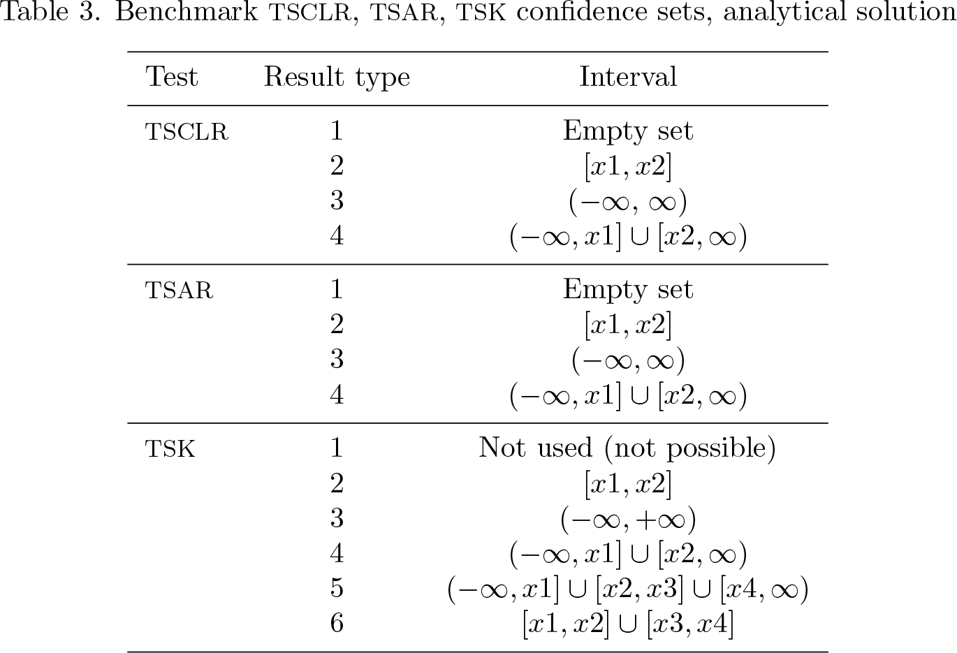
The confidence sets have correct coverage in the limit because they are inverted from asymptotically valid tests under the weak IV asymptotics. When the instruments are weak, the confidence sets could be unbounded, which is an essential property for confidence sets to have correct coverage with arbitrarily weak instruments (Dufour 1997). The benchmark confidence sets are computed analytically following the fastcomputation method proposed by Mikusheva and Poi (2006) for the classic (one-sample) Anderson–Rubin, K, and conditional likelihood-ratio confidence sets.

Like the classic K test, the TSK test also has an irregular nonmonotonic power curve when k ≥ 2, resulting in power loss with some DGPs. For confidence sets, TSK can take the form of a union of two finite intervals, that is, [x ₁ , x ₂] ∪ [x ₃ , x ₄], while TSAR and TSCLR confidence sets, conditional on boundedness, take only the usual form of a finite interval, or [x ₁ , x ₂]. Therefore, as with the classic one-sample case (see, for example, Mikusheva and Poi [2006]), the TSK method is generally not recommended in practice.

Table 2 is taken from panels A and B of table 1 in Choi, Gu, and Shen (2018). It uses the same DGP as the one discussed in section 2. Compared with the TS2SLS results reported in table 1, the proposed TSAR, TSCLR, and TSK confidence sets have targeted coverage rates regardless of instrument strength. Panel B of table 2 provides a rough idea about how often the proposed weak-instrument robust confidence sets could be unbounded given various instrument strengths. The panel also shows good power performance of TSCLR and irregular power performance of TSK under some DGPs.

Table 2.

Properties of benchmark weak-instrument robust confidence sets

	TSAR			TSCLR			TSK
λ/k	1	4	16	1	4	16	1	4	16
Panel A: coverage of 95% confidence sets
(a): β = −2
k = 1	0.947	0.955	0.947	0.947	0.955	0.947	0.947	0.955	0.947
k = 5	0.951	0.950	0.952	0.958	0.950	0.954	0.957	0.949	0.954
k = 10	0.948	0.944	0.943	0.946	0.944	0.950	0.947	0.945	0.950
(b): β = 0
k = 1	0.947	0.946	0.948	0.947	0.946	0.948	0.947	0.946	0.948
k = 5	0.947	0.955	0.952	0.950	0.949	0.946	0.953	0.950	0.946
k = 10	0.948	0.945	0.949	0.954	0.948	0.949	0.957	0.948	0.948
(c): β = 2
k = 1	0.946	0.951	0.950	0.946	0.951	0.950	0.946	0.951	0.950
k = 5	0.951	0.948	0.950	0.959	0.951	0.954	0.960	0.950	0.953
k = 10	0.952	0.945	0.944	0.949	0.949	0.946	0.949	0.949	0.946
Panel B: number of bounded 95% confidence sets among 5,000 simulations
(a): β = −2
k = 1	854	2,648	4,901	854	2,648	4,901	854	2,648	4,901
k = 5	1,730	4,635	4,872	2,670	4,963	5,000	2,649	4,964	5,000
k = 10	2,525	4,818	4,811	4,075	5,000	5,000	4,032	5,000	5,000
(b): β = 0
k = 1	854	2,648	4,901	854	2,648	4,901	854	2,648	4,901
k = 5	1,804	4,682	4,874	1,732	4,712	5,000	843	2,116	3,419
k = 10	2,633	4,849	4,838	2,500	4,983	5,000	857	2,025	3,275
(c): β = 2
k = 1	854	2,648	4,901	854	2,648	4,901	854	2,648	4,901
k = 5	1,734	4,639	4,879	2,667	4,960	5,000	2,629	4,962	5,000
k = 10	2,546	4,816	4,812	4,066	4,999	5,000	4,014	4,999	5,000

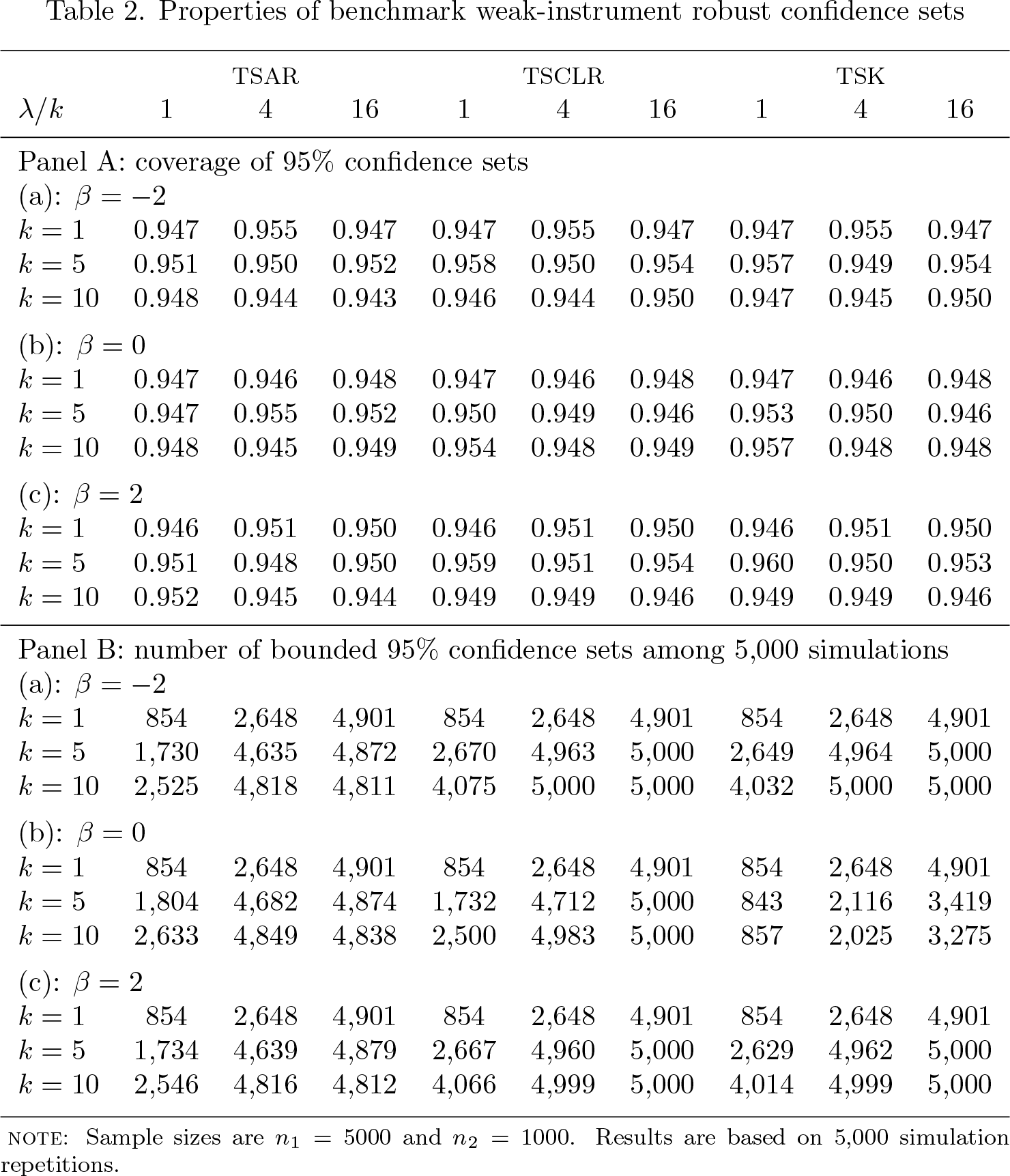
Note: Sample sizes are n₁ = 5000 and n₂ = 1000. Results are based on 5,000 simulation repetitions.

3.2 Fully robust tests and confidence sets

This section relaxes the assumptions of homoskedasticity and equal moments of excluded instruments and exogenous regressors. Let Σ _z,u ₁ and Σ _z, _ε2 be probability limits of $V ({Z^{'}}_{1} u_{1} / \sqrt{n_{1}})$ and $V ({Z^{'}}_{2} ε_{2} / \sqrt{n_{2}})$ , respectively, and let Σ _l,ZZ be the probability limit of Z l ^′ Z _l/n_l for l = 1, 2. Replace the first equation in the two-sample IV regression model with its reduced form y ₁ = Z ₁ζ + X ₁γ + u ₁. Let δ = [ζ π]^′. We know that

r (δ, β) = ζ - π β = 0

Let $\hat{ζ} = {({Z^{'}}_{1} Z_{1})}^{-1} Z^{'} y_{1}, \hat{π} = {({Z^{'}}_{2} Z_{2})}^{-1} Z^{'} w_{2}$ and $\hat{δ} = {[\hat{ζ} \hat{π}]}^{'}$ . It is easy to see that, for any β ₀,

\sqrt{n_{1}} {r (\hat{δ}, β_{0}) - r (δ, β_{0}) \Rightarrow N (0, Σ_{β_{0}})

where $\sum β_{0} = \sum_{1,}^{- 1} Z Z \sum_{Z, u_{1}} \sum_{1, Z Z}^{- 1} + τ β_{0}^{2} \sum_{2, Z Z}^{- 1} \sum_{Z},_{\in_{2}} \sum_{2, Z Z}^{- 1}$ is a k × k variance–covariance matrix. Let $\hat{Σ} b_{ζ, β_{0}} = {n_{1}^{2} / (n_{1} - k - p)} {({Z^{'}}_{1} Z_{1})}^{- 1} (\sum_{i = 1}^{n_{1}} {\hat{u}}_{1 i}^{2} Z_{1 i} {Z^{'}}_{1 i}) {({Z^{'}}_{1} Z_{1})}^{- 1}$ and let ${\sum^{^}}_{π, β_{0}} = {n_{2}^{2} / (n_{2} - k - p)} {({Z^{'}}_{2} Z_{2})}^{- 1} (\sum_{i = 1}^{n_{2}} {\hat{ε}}_{2 i}^{2} Z_{2 i} {Z^{'}}_{2 i}) {({Z^{'}}_{2} Z_{2})}^{- 1}$ , where ${\hat{u}}_{1 i}$ is the ith entry of $M_{[Z_{1} : X_{1}]} y_{1}$ and ${\hat{ε}}_{2 i}$ is the ith entry of $M_{[Z_{2} : X_{2}]} w_{2}$ . Then $\sum_{β_{0}}$ could be consistently estimated by ${\hat{Σ}}_{β_{0}} = {\hat{Σ}}_{ζ, β_{0}} + (n_{1} / n_{2}) β_{0}^{2} {\hat{Σ}}_{π, β_{0}}$ .

Following Magnusson (2010), the robust TSAR, TSK, and TSCLR test statistics for H ₀: β = β ₀ can be written as

\begin{array}{l} T_{1, robust} (β_{0}) = n_{1} {(\hat{ζ} - \hat{π} β_{0})}^{'} {\sum^{^}}_{β_{0}}^{- 1} (\hat{ζ} - \hat{π} β_{0}) \\ T_{2, robust} (β_{0}) = n_{1} {{\sum^{^}}_{β_{0}}^{- 1 / 2} (\hat{ζ} - \hat{π} β_{0})}^{'} P_{{\sum^{^}}_{β_{0}}^{- 1 / 2} {\hat{D}}_{β_{0}}} {{\sum^{^}}_{β_{0}}^{- 1 / 2} (\hat{ζ} - \hat{π} β_{0})} \\ T_{3, robust} (β_{0}) = \frac{1}{2} [T_{1, robust} {\hat{q}}_{β_{0}} + {{(T_{1, robust} {\hat{q}}_{β_{0}})}^{2} - 4 (T_{1, robust} {\hat{q}}_{β_{0}} - T_{2, robust} {\hat{q}}_{β_{0}})}^{1 / 2}] \end{array}

where $- {\hat{D}}_{β_{0}} = \hat{π} + (n_{1} / n_{2}) β_{0} {\hat{Σ}}_{π, β_{0}} {\hat{Σ}}_{β_{0}}^{- 1} (\hat{ζ} - \hat{π} β_{0})$ and $\hat{q} β_{0} = n_{1} {\hat{D}}^{'}_{β_{0}} {(n_{1} / n_{2}) {\hat{Σ}}_{π, β_{0}} - {(n_{1} / n_{2})}^{2} β_{0}^{2} {\hat{Σ}}_{π, β_{0}} {\hat{Σ}}_{β_{0}}^{- 1} {\hat{Σ}}_{π, β_{0}}}^{- 1} {\hat{D}}_{β_{0}}$ . When the robust variance–covariance matrix ${\hat{Σ}}_{β_{0}}$ is replaced with ${\bar{Σ}}_{β_{0}} = {\hat{σ}}_{u_{1}}^{2} {({Z^{'}}_{1} Z_{1}) / n_{1}}^{- 1} + (n_{1} / n_{2}) β_{0}^{2} {({Z^{'}}_{1} Z_{1}) / n_{1}}^{- 1} {\hat{σ}}_{ε_{2}}^{2}$ , the three robust test statistics reduce to the benchmark counterparts.

Under the null hypothesis, T _1,robust(β ₀) and T _2,robust(β ₀) have limiting distributions χ ²(k) and χ ²(1), respectively, and T _3,robust(β ₀) ⇒ (1/2)(χ ²(1)+χ ²(k−1)−q _β0+[{χ ²(1)+ χ ²(k − 1) + q _β0}² − 4χ ²(k − 1)q _β0]^1/2), where χ ²(1) and χ ²(k − 1) are independent chisquared distributed random variables with 1 and k − 1 degrees of freedom, respectively, given that ${\hat{q}}_{β_{0}} = q_{β_{0}}$ . Therefore, we reject the null if T _1,robust(β ₀) is larger than q _1−α(k), if T _2,robust(β ₀) is larger than q _1−α(1), or if p(T _3,robust(β ₀); ${\hat{q}}_{β_{0}}$ ) is smaller than α, where p(.; .) is defined in section 3.1.

As with the benchmark case, one can construct robust TSAR, TSK, and TSCLR confidence sets of β by inverting the robust TSAR, TSK, and TSCLR tests. In the proposed command, these fully robust confidence sets are computed using a grid search. Specifically, we wrote our grid search codes based on the ivtest command developed by Finlay and Magnusson (2009). We omitted simulation results for the robust TSAR, TSK, and TSCLR tests and confidence sets. Interested readers can refer to the simulation section in Choi, Gu, and Shen (2018) for details. Like the benchmark case, the robust TSAR, TSK, and TSCLR methods have good size and coverage properties regardless of the strength of instruments.

4 Implementation

By default, the weaktsiv command generates two output tables. The first table reports TS2SLS estimates together with Inoue and Solon (2010) standard errors. The second table calculates the benchmark TSAR, TSK, and TSCLR tests and confidence sets discussed in section 3.1. If the robust option is used, the weaktsiv command provides TS2SLS estimates together with Pacini and Windmeijer (2016) standard errors, as well as the robust TSAR, TSK, and TSCLR tests and confidence sets discussed in section 3.2.

The two-sample IV regression model requires the use of two data samples. weaktsiv distinguishes the two samples based on missing values of outcome and endogenous variables. If the dataset has nonmissing values in both outcome and endogenous variables, weaktsiv drops these observations.

4.1 Syntax

weaktsiv depvar varlist_exog ( varlist_endog = varlist_iv ) [if] [in] [, nocons robust level( # ) test( # ) points( # ) grid( # ( # ) # )]

depvar is the outcome variable.

varlist_exog is the list of exogenous variables.

varlist_endog is the endogenous regressor of the model.

varlist_iv is the list of exogenous variables used together with varlist_exog as instruments for varlist_endog.

4.2 Options

nocons suppresses the constant term in the regression model.

robust provides versions of two-sample weak IV robust tests that are also robust to heteroskedasticity and unequal moments of excluded instruments and exogenous regressors across the two data samples. robust also reports Pacini and Windmeijer’s (2016) robust standard error following the TS2SLS estimation.

level( # ) sets the confidence level. The default is level(95).

test( # ) sets the hypothesized value of the endogenous variable’s coefficient. The default is test(0).

points( # ) specifies the number of points used to create the grid for confidence region calculation. points()may be used together only with the robust option and cannot be used together with the grid() option. The default is points(100).

grid( # ( # ) # ) specifies the grid used for confidence region calculation. grid() may be used together only with the robust option because the benchmark confidence regions are calculated analytically. The default uses the TS2SLS estimator plus or minus two times the Pacini and Windmeijer (2016) standard error and 100 grid points.

4.3 Stored results

weaktsiv stores the following in e():

For the benchmark methods, the stored type (that is, e(TSAR_type), e(TSK_type), and e(TSCLR_type)) and endpoints (that is, e(TSAR_xi), e(TSK_xi), and e(TSCLR_xi)) can be used together to retrieve the exact confidence sets using the relationship in table 3.

Table 3.

Benchmark TSCLR, TSAR, TSK confidence sets, analytical solution

Test	Result type	Interval
TSCLR	1	Empty set
	2	[x1, x2]
	3	(−∞, ∞)
	4	(−∞, x1] ∪ [x2, ∞)
TSAR	1	Empty set
	2	[x1, x2]
	3	(−∞, ∞)
	4	(−∞, x1] ∪ [x2, ∞)
TSK	1	Not used (not possible)
	2	[x1, x2]
	3	(−∞, +∞)
	4	(−∞, x1] ∪ [x2, ∞)
	5	(−∞, x1] ∪ [x2, x3] ∪ [x4, ∞)
	6	[x1, x2] ∪ [x3, x4]

5 Example

5.1 The case with just-identification

We use the dataset of Currie and Yelowitz (2000) to illustrate implementing the command weaktsiv in the case of just-identification. The example estimates the effects of public housing on monthly rental payments in equations (2) and (3) of Currie and Yelowitz (2000). The outcome variable is household monthly rental payments (ry1). The endogenous regressor is a dummy variable indicating whether a household participates in the public housing project (ry2). The excluded instrument is the sex composition of children, a dummy variable equaling one if the family has a boy and a girl (z). The exogenous regressors include information on the household head’s age and its square, marital status, sex, race, education level, metropolitan statistical area-level controls for public housing supply, and children’s sex.

The default weaktsiv command gives a table reporting the TS2SLS estimation results together with Inoue and Solon (2010) standard errors and another table reporting benchmark TSCLR results. Only TSCLR is reported here because TSAR, TSK, and TSCLR are equivalent when the model is just-identified.

For the effects of public housing on monthly rental payments, the CI based on Inoue and Solon (2010) standard errors is [0.151, 0.592]. The weak-instrument robust CI is [0.214, 0.784], which is wider than the nonrobust one. The TSCLR CI is also centered farther away from zero than the TS2SLS CI likely because TS2SLS suffers from an attenuation bias and is biased toward zero. These CI results are also reported in column 1 of table 3 in Choi, Gu, and Shen (2018). The TSCLR CI reported here is slightly different from the one reported in Choi, Gu, and Shen (2018) because of different rounding methods in the two articles. R codes for the empirical applications in Choi, Gu, and Shen (2018) kept three significant digits after the decimal point for benchmark weak-IV robust confidence sets and two significant digits the fully robust confidence sets.

We emphasize that both CIs reported by the default command require the assumptions of homoskedasticity and equal moments. Next, we illustrate the use of the robust option. With this option, the weaktsiv command reports inference results that are robust to both heteroskedasticity and unequal moments of excluded instruments and exogenous regressors. The TS2SLS output table now reports Pacini and Windmeijer (2016) standard errors. The weak IV robust output table reports results from the fully robust version of TSAR, TSK, and TSCLR. Again, in this example, only TSCLR is reported because of just-identification. The robust TSCLR CI is also [0.214, 0.784].

5.2 The case with overidentification

Now we illustrate the weaktsiv command in the case of overidentification. We use the dataset of Olivetti and Paserman (2015), who examine historical intergenerational income elasticity in the United States. We consider the specification in column 1, row 5, in table 3 of Olivetti and Paserman (2015) for father–son-in-law elasticity in 1950–1970. The outcome variable of interest is a son-in-law’s log earnings (ry1). The endogenous regressor is a father’s log earnings (ry2). The excluded instruments are dummy variables for a daughters’ first name (z1–z726). There are no exogenous regressors in the model except for the intercepts.

The following outputs are from the default setting of the weaktsiv command, which reports TS2SLS estimates with Inoue and Solon (2010) standard errors as well as benchmark TSAR, TSK, and TSCLR tests and confidence sets. The results are also reported in column 1, row 5, in table 2 of Choi, Gu, and Shen (2018). The Inoue and Solon (2010) CI is [0.307, 0.401], while the benchmark TSCLR CI is [0.571, 0.731]. Again, the TSCLR CI lies above the TS2SLS CI likely because of the large attenuation bias of TS2SLS: TS2SLS has only a first-stage F statistic equal to 1.98.

As discussed in Choi, Gu, and Shen (2018), the empirical example of Olivetti and Paserman (2015) is not suitable for heteroskedasticity-robust inference because their regression specifications result in perfect fit for a number of observations in either the first-stage or the reduced-form regressions. Therefore, heteroskedasticity-robust inference cannot be carried out for either TS2SLS or the proposed weak-instrument robust methods. To illustrate the use of our robust option in models with overidentification, we turn back to the Currie and Yelowitz (2000) example discussed in section 5.1. We randomly generate a normally distributed instrument and use it as the second instrument (z2). This overidentified model generates results close to those reported in section 5.1 for TS2SLS as well as robust TSCLR and TSK. Robust TSAR CI is a little wider in length because TSAR is generally inefficient when the number of instruments exceeds the number of endogenous regressors.

6 Programs and supplemental materials

Supplemental Material, st0568 - Two-sample instrumental-variables regression with potentially weak instruments

Supplemental Material, st0568 for Two-sample instrumental-variables regression with potentially weak instruments by Jaerim Choi and Shu Shen in The Stata Journal

Footnotes

6 Programs and supplemental materials

To install a snapshot of the corresponding software files as they existed at the time of publication of this article, type

References

Andrews

D. W. K.

Moreira

M. J.

Stock

J. H.

2006. Optimal two-sided invariant similar tests for instrumental variables regression. Econometrica 74: 715–752.

Andrews

D. W. K.

Moreira

M. J.

Stock

J. H.

2007. Performance of conditional Wald tests in IV regression with weak instruments. Journal of Econometrics 139: 116–132.

Andrews

D. W. K.

Moreira

M. J.

Stock

J. H.

2008. Efficient two-sided nonsimilar invariant tests in IV regression with weak instruments. Journal of Econometrics 146: 241–254.

Angrist

J. D.

Krueger

A. B.

1992. The effect of age at school entry on educational attainment: An application of instrumental variables with moments from two samples. Journal of the American Statistical Association 87: 328–336.

Angrist

J. D.

Krueger

A. B.

1995. Split-sample instrumental variables estimates of the return to schooling. Journal of Business & Economic Statistics 13: 225–235.

Björklund

Jäntti

1997. Intergenerational income mobility in Sweden compared to the United States. American Economic Review 87: 1009–1018.

Bound

Jaeger

D. A.

Baker

R. M.

1995. Problems with instrumental variables estimation when the correlation between the instruments and the endogeneous explanatory variable is weak. Journal of the American Statistical Association 90: 443–450.

Brunner

E. J.

Cho

S.-W.

Reback

2012. Mobility, housing markets, and schools: Estimating the effects of inter-district choice programs. Journal of Public Economics 96: 604–614.

Choi

Shen

2018. Weak-instrument robust inference for two-sample instrumental variables regression. Journal of Applied Economics 33: 109–125.

10.

Currie

Yelowitz

2000. Are public housing projects good for kids? Journal of Public Economics 75: 99–124.

11.

Dufour

J.-M.

1997. Some impossibility theorems in econometrics with applications to structural and dynamic models. Econometrica 65: 1365–1387.

12.

Dufour

J.-M.

Jasiak

2001. Finite sample limited information inference methods for structural equations and models with generated regressors. International Economic Review 42: 815–844.

13.

Feldman

N. E.

2010. Mental accounting effects of income tax shifting. Review of Economics and Statistics 92: 70–86.

14.

Finlay

Magnusson

L. M.

2009. Implementing weak-instrument robust tests for a general class of instrumental-variables models. Stata Journal 9: 398–421.

15.

Inoue

Solon

2010. Two-sample instrumental variables estimators. Review of Economics and Statistics 92: 557–561.

16.

Kleibergen

2002. Pivotal statistics for testing structural parameters in instrumental variables regression. Econometrica 70: 1781–1803.

17.

Magnusson

L. M.

2010. Inference in limited dependent variable models robust to weak identification. Econometrics Journal 13: S56–S79.

18.

Miguel

2005. Poverty and witch killing. Review of Economic Studies 72: 1153–1172.

19.

Mikusheva

Poi

B. P.

2006. Tests and confidence sets with correct size when instruments are potentially weak. Stata Journal 6: 335–347.

20.

Moreira

M. J.

2003. A conditional likelihood ratio test for structural models. Econometrica 71: 1027–1048.

21.

Moreira

M. J.

2009. Tests with correct size when instruments can be arbitrarily weak. Journal of Econometrics 152: 131–140.

22.

Olivetti

Paserman

M. D.

2015. In the name of the son (and the daughter): Intergenerational mobility in the United States, 1850–1940. American Economic Review 105: 2695–2724.

23.

Pacini

Windmeijer

2016. Robust inference for the two-sample 2SLS estimator. Economics Letters 146: 50–54.

24.

Siminski

2013. Employment effects of army service and veterans’ compensation: Evidence from the Australian Vietnam-era conscription lotteries. Review of Economics and Statistics 95: 87–97.

25.

Staiger

Stock

J. H.

1997. Instrumental variables regression with weak instruments. Econometrica 65: 557–586.

Supplementary Material

Please find the following supplemental material available below.

For Open Access articles published under a Creative Commons License, all supplemental material carries the same license as the article it is associated with.

For non-Open Access articles published, all supplemental material carries a non-exclusive license, and permission requests for re-use of supplemental material or any part of supplemental material shall be sent directly to the copyright owner as specified in the copyright notice associated with the article.

0.98 MB

0.00 MB