Sage Journals: Discover world-class research

Abstract

We introduce two commands, nstagebin and nstagebinopt, that can be used to facilitate the design of multiarm multistage (MAMS) trials with binary outcomes. MAMS designs are a class of efficient and adaptive randomized clinical trials that have successfully been used in many disease areas, including cancer, tuberculosis, maternal health, COVID-19, and surgery. The nstagebinopt command finds a class of efficient “admissible” designs based on an optimality criterion using a systematic search procedure. The nstagebin command calculates the stagewise sample sizes, trial timelines, and overall operating characteristics of MAMS designs with binary outcomes. Both commands allow the use of Dunnett’s correction to account for multiple testing. We also use the ROSSINI 2 MAMS design, an ongoing MAMS trial in surgical wound infection, to illustrate the capabilities of both commands. The new commands facilitate the design of MAMS trials with binary outcomes where more than one research question can be addressed under one protocol.

Keywords

st0728 nstagebin nstagebinopt multiarm multistage MAMS familywise type I error rate FWER adaptive designs

1 Introduction

Randomized controlled trials are the gold standard for testing whether a new treatment is better than the current standard of care. Multiarm multistage (MAMS) trial designs are efficient adaptive designs that have been proposed to speed up the evaluation of new therapies and improve success rates in identifying effective ones (Parmar et al. 2008). The MAMS design achieves this goal with two main components: The multiarm aspect allows multiple experimental arms to be compared with a common control (which is generally taken as the current standard of care) in one trial, and the multistage aspect allows interim analyses before the planned end of the study. This enables us to cease recruitment early to potentially inefficacious experimental arms or stop early for the overwhelming efficacy. This allows multiple research questions to be efficiently answered under the same protocol.

Royston, Parmar, and Qian (2003) and Royston et al. (2011) developed a MAMS design for trials with time-to-event outcomes that uses an intermediate (I) outcome at interim stages. This increases the efficiency of the MAMS design further because it allows for the earlier stopping of treatment arms for lack of benefit at interim stages while maintaining a low probability of false negatives (that is, 1 − power). In this framework, the information on the I outcome accrues at the same or a faster rate than information for the definitive (D) or primary outcome of the trial. The I outcome should be on the causal pathway to D, but it does not necessarily have to be a surrogate outcome (Parmar et al. 2008). If there is no effect of treatment on I, then it is highly desirable that the same holds for D; otherwise, there is an increased risk of wrongly stopping a study early for lack of benefit. Choodari-Oskooei et al. (2022) give an extensive account of Royston, Parmar, and Qian (2003) and Royston et al.’s (2011) MAMS designs and discuss their underlying principles.

Examples of intermediate and primary outcomes are progression-free (or diseasefree) survival and overall survival for many cancer trials, CD4 count and disease-specific survival for HIV trials, or culture status (a binary marker for whether a patient has tuberculosis) and patient relapse (binary) in tuberculosis trials. When one uses an I outcome, each of the experimental arms is compared pairwise with the control arm on the I outcome. In the absence of an obvious choice for I, a rational choice of I might be D itself earlier in time. In this article, the MAMS designs that use the I outcome for the lack-of-benefit analysis at the interim looks are denoted by I ≠ D. Designs that use the same primary outcome at the interim looks are denoted by I = D. Throughout, we use the acronym MAMS to refer to the multiarm multistage design described by Royston, Parmar, and Qian (2003) and Royston et al. (2011).

Binary (or dichotomous) outcomes are widely used in many clinical studies. The MAMS design has been extended to binary outcomes with the risk difference as the primary outcome measure (see Bratton, Phillips, and Parmar [2013]) and can easily be extended to designs with the log odds-ratio as the primary outcome measure (Abery and Todd 2018). It is one of the few adaptive designs being deployed both in several trials and across a range of diseases, including trials in COVID-19, cancer, tuberculosis, and surgery. One example is the MAMS ROSSINI 2 trial in surgical site infection (SSI), which is used in this article as an example and for illustration (ROSSINI 2 2023).

The purpose of this article is twofold. First, it introduces two commands, nstagebin and nstagebinopt, that facilitate the design of MAMS trials with binary outcomes. Second, it addresses the problem of how to find efficient MAMS trials with particular pairwise or familywise operating characteristics. The nstagebin command operates similarly to nstage (Barthel, Royston, and Parmar 2009) for time-to-event outcomes. Given a set of design parameters (including the number of arms, stages, target risk differences, stagewise significance levels, and powers), nstagebin calculates the required sample sizes for the analysis at the end of each stage in addition to stage durations and the overall pairwise type I error rates and familywise type I error rates (FWER). The nstagebinopt command finds a class of efficient “admissible” designs based on an optimality criterion that has been introduced for adaptive designs using a systematic search procedure. It finds a large set of feasible designs—that is, a design with a particular (prespecified) overall type I error rate and power—and selects those that minimize the given optimality criteria. In designs that require correction for multiplicity, both commands apply Dunnett’s (1955) correction to account for multiple testing due to multiple experimental arms. We use the ROSSINI 2 MAMS trial as an example to describe the sample-size calculations and capabilities of these commands. The ROSSINI 2 MAMS trial uses the same primary outcome at all stages of the trial, that is, the I = D design. In appendix A of the online supplementary material, we also include an example MAMS trial design that uses an intermediate (binary) outcome at interim stages, which is different from that of the primary outcome at the final analysis (Bratton, Phillips, and Parmar 2013).

The structure of this article is as follows. Section 2 presents the specification of the MAMS design with binary outcomes. It also describes a class of efficient admissible MAMS designs in section 2.3 and introduces a flexible family of α functions to allow for a larger set of such designs to be found. Sections 3 and 4 present the nstagebin and nstagebinopt syntax and dialog boxes. Section 5 describes how to define design parameters in nstagebin and shows the outputs of both commands using the ROSSINI 2 trial as an example. Finally, we discuss our findings.

2 MAMS designs with binary outcomes

This section presents the specification of the MAMS design with binary outcomes. For a MAMS trial with K experimental arms and J stages, parameters π_jk and π_j ₀ are the risks of developing the outcome of interest at stage j in an experimental arm k and the control arm, respectively. The treatment effect is the difference in risks, that is, a reduction in an unfavorable event rate, and is being measured by θ_jk = π_jk − π_j ₀, where j = 1,…, J and k = 1,…, K. For simplicity, because we assume that all K pairwise comparisons have the same design parameters (that is, all have the same design stagewise significance level α_j and power ω_j ), we remove the subscript k from the notations of design parameters.

Without loss of generality, assume that a negative value of θ_jk indicates a beneficial effect of treatment k. In trials with K experimental arms, where a set of K null hypotheses are tested at each stage j, the null and alternative hypotheses are

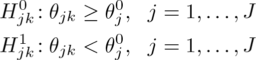
\begin{array}{l} H_{j k}^{0} : θ_{j k} \geq θ_{j}^{0}, j = 1, \dots, J \\ H_{j k}^{1} : θ_{j k} < θ_{j}^{0}, j = 1, \dots, J \end{array}

for some prespecified (design) null effects $θ_{j}^{0}$ . In practice, $θ_{j}^{0}$ is usually taken to be 0 on the absolute risk difference. If the same definitive (D) outcome is monitored throughout the trial (I = D designs), the true treatment effect (θ_jk ) and $θ_{j}^{0}$ are assumed constant for all j. Otherwise, θ_Jk and $θ_{J}^{0}$ correspond to the true and null effects on the definitive outcome and θ_jk and $θ_{j}^{0}$ correspond to the intermediate outcome for all j < J and are constant. For sample-size and power calculations, a minimum target treatment effect (often the minimum clinically important risk difference) is also required, that is, $θ_{j}^{1}$ . The MAMS framework can be applied to both superiority and noninferiority (NI) designs where the aim is to show that the active arm is not worse than control by the prespecified NI margin—see appendix A of the online supplementary material for an example with the NI design and how to define the null and alternative hypotheses in this setting.

At each stage, we define the design significance level α = (α ₁ ,…, α_J ) and power ω = (ω ₁ ,…, ω_J ) for testing each pairwise comparison. Let Z_jk be the z test statistic comparing experimental arm k against the control arm at stage j, where Z_jk follows a standard normal distribution, Z_jk ∼ N(0, 1), under the null hypothesis. Note that all the cumulative data from previous stages are used in the calculations of each z test statistic. In other words, the pairwise analyses at each stage includes all the individuals that were included in the analyses of previous stages. The joint distribution of the z test statistics therefore follows a multivariate normal distribution with the location parameter as the J × K matrices of the standardized mean treatment effects and the corresponding covariance matrix (Σ) between the J × K test statistics. Note that the Fisher’s (observed) information (V_jk ) contained in ${\hat{θ}}_{j k}$ is defined as {V_jk = 1/Var $({\hat{θ}}_{j k})$ }. At each interim analysis j = 1,…, J −1, the treatment-effect estimates and their corresponding test statistics (Z_j ₁ ,…, Z_jk ) are calculated together with their corresponding p-values (p_jk ).

If p_jk ≥ α_j , the result for the pairwise comparison of experimental arm k against the control arm crosses the jth interim lack-of-benefit stopping rule; therefore, recruitment to that experimental arm can be stopped for lack of benefit.

If p_jk < α_j , continue recruitment in the experimental arm k and control arm and move to the next stage.

At the final analysis J, the treatment effect is estimated on the primary (D) outcome for each experimental arm and includes all the randomized individuals from previous stages in comparison k. As a result, one of two conclusions can be made:

If p_Jk ≤ α_J , reject the null hypothesis corresponding to the definitive outcome and claim efficacy.

If p_Jk ≥ α_J , the corresponding null hypothesis cannot be rejected.

2.1 Steps to design a MAMS trial with a binary outcome

The MAMS design requires the specification of the following design parameters to calculate the sample size and trial duration for each stage (j): the (stagewise) design power (ω_j ) and significance levels (α_j ); the allocation ratio, which is the number of randomized individuals in each experimental arm for every individual that is randomized to the control arm (A); the target effect size under the null ( $θ_{j}^{0}$ ) and alternative ( $θ_{j}^{1}$ ) hypotheses; the number of arms and stages; and the stagewise accrual rate and the control-arm event rate for the D and (in I ≠ D designs) I outcomes. Below, we outline the steps to design a MAMS trial with binary outcomes:

Choose the number of experimental (E) arms, K, and stages, J.

Choose the definitive D outcome and (optionally, in I ≠ D designs) the I outcome.

Choose the null values for the underlying treatment effect, θ—for example, the difference in risks on the definitive and (in I ≠ D designs) intermediate outcomes.

Choose the minimum clinically relevant target treatment-effect size, $θ_{j}^{1}$ .

Choose the control-arm event rate.

Choose the allocation ratio A (E:C), the number of patients allocated to each experimental arm for every patient allocated to the control arm. For a fixed sample (one-stage) multiarm trial, the optimal allocation ratio (that is, the one that minimizes the sample size for a fixed power) is approximately $A = 1 / \sqrt{K}$ .

In I ≠ D designs, choose an estimate of the probability of experiencing the definitive (final) outcome given the patient has had the intermediate outcome—that is, the positive predictive value (PPV)—for the control arm and for experimental arms. This allows us to estimate the correlation between the treatment effect on the intermediate outcome and that of the definitive outcome to calculate the overall pairwise power. An estimate of the PPV can be obtained using data from previous trials, through expert opinion, or both—more information is included in Bratton, Phillips, and Parmar (2013). In the ROSSINI 2 design, the same outcome was used at interim stages (that is, I = D design), so this was not required—see appendix A in the online supplemental material for a trial example with I ≠ D design.

Choose the accrual rate per stage (and optionally, loss to follow-up) to calculate the trial timelines. The nstagebin command also has two other related options (extrat() and fu()) that can be invoked to allow for the minimum follow-up period to observe the outcomes or the extra time that is needed for data cleaning, analysis, and the various committee meetings that are usually required.

Choose a one-sided design significance level for lack of benefit and the target power for each stage (α_j , ω_j ). The chosen values for α_j and ω_j are used to calculate the required sample sizes for each stage.

The nstagebinopt command can be used to determine these values—see sections 2.3 and 4. Generally, larger-than-traditional (more permissive) values of α_j are used at the interim stages because a decision can be made on dropping or continuing arms reasonably early, that is, with a relatively small sample size. Furthermore, the power in the intermediate stages of the trial should ideally be at least as high as the final-stage power to give effective experimental arms a stronger chance of reaching the planned end of the trial, thus allowing more data to be collected for these arms: ω_j ≥ ω_J for all j = 1,…, J − 1. This will give effective arms a stronger chance of reaching the final stage, thus allowing more data to be collected on them.

2.2 Type I error rate and power

In trials with lack-of-benefit interim stopping boundaries, a type I error is made only if the null hypothesis for the D outcome is rejected in final-stage analysis. In designs with J stages and stopping boundaries for lack of benefit, Royston et al. (2011) showed that, in I = D designs, the overall pairwise type I error rate, α, and power, ω, for each of the k pairwise comparisons are calculated from

\begin{array}{l} α = Φ_{J} (z_{α_{1}}, \dots, z_{α_{J}}; R_{J}^{0}) & under θ_{j} = θ_{j}^{0} for all j \\ ω = Φ_{J} (z_{ω_{1}}, \dots, z_{ω_{J}}; R_{J}^{1}) & under θ_{j} = θ_{j}^{1} for all j \end{array}

where Φ _J is the J-dimensional multivariate normal distribution function with correlation matrix $R_{J}^{0 / 1}$ . The (j, j′)th entry of R is the correlation between the treatment effects in stages j and j′—formulas are given in Bratton, Phillips, and Parmar (2013).

In I ≠ D designs, the calculation of α in (1) is made under the assumption that H ₀ is true for both I and D. However, in this case the type I error rate is maximized when the experimental treatment is highly or infinitely effective on I but the null hypothesis is true for D. Therefore, the maximum pairwise type I error rate, α _max, is equal to the final-stage significance level, α_J (Bratton et al. 2016).

In multiarm trials, there are multiple ways to commit a type I error. In some trials such as the ROSSINI 2 trial, it is required to control the overall FWER at a prespecified level, usually at 2.5% (one sided). The FWER is the probability of incorrectly rejecting the null hypothesis for the primary outcome for at least one of the experimental arms from a set of comparisons in a multiarm trial. The FWER is maximized under the global null hypothesis, $H_{0}^{G}$ , that is, when the null hypothesis that maximizes pairwise alpha is true for all arms. It is therefore calculated under this hypothesis (Bratton et al. 2016).

2.3 Admissible MAMS designs

In Royston, Parmar, and Qian (2003) and Royston et al.’s (2011) framework, a MAMS design is constructed by specifying a one-sided significance level and power for the pairwise comparisons at each stage of the study along with the minimum target treatment effect for the outcome of interest in that stage and the allocation ratio for the trial. Given these design parameters, the sample size required for each analysis is calculated. The (one-sided) design significance levels act as the stopping boundaries for lack of benefit. Previous MAMS trials such as the STAMPEDE trial (Sydes et al. 2012) have used the recommendations given by Royston et al. (2011) to choose the stagewise significance levels and powers.

Royston et al. (2011) suggested using high power in the intermediate stages (for example, 0.95) and also the final stage (for example, 0.90) to ensure high overall power for the trial. They also suggested using a descending geometric sequence such as α_j = 0.5 ^j for the significance levels in the intermediate stages. However, this approach is problematic for two main reasons. First, it may not result in a “feasible” design with the desired overall operating characteristics. To achieve this, a time-consuming trial-anderror approach is required in which users must continually tweak the stagewise (design) operating characteristics until a feasible design with the desired overall operating characteristics is found. Second, there are likely to be many feasible designs for any pair of overall operating characteristics, some requiring smaller sample sizes than others. Therefore, the chosen design may not be the most efficient or optimal for a particular true treatment effect. Thus, the most efficient feasible MAMS design for a particular study is unlikely to be found if this approach is used for trial design.

To address these difficulties, Bratton (2015) developed a systematic grid-search procedure over the stagewise significance levels and power to find a large set of feasible designs, that is, designs with a particular (prespecified) overall type I error rate and power. The procedure then selects the most efficient feasible designs, called admissible MAMS designs, using an optimality criteria proposed by Jung et al. (2004), which is a weighted sum of the expected sample size under the global null hypothesis, E(N|H ₀), and the hypothesis in which all arms are effective, E(N|H ₁):

L (q) = q E (N ∣ H_{1}) + (1 - q) E (N ∣ H_{0})

Feasible designs that minimize (2) for some q ∊ [0, 1] are called admissible. Note that the user chooses q based on the prior beliefs about the effectiveness of the treatment under study. Special cases are the null-optimal design with q = 0, which minimizes the expected sample size under the global null hypothesis, that is, E(N|H ₀), and minimax designs with q = 1, which minimizes E(N|H ₁). However, other admissible designs that minimize a more balanced weighting of the two measures exist. Jung et al. (2004) found that these “balanced” admissible designs are often much more appealing in practice because they usually possess similar desirable properties to the null-optimal or minimax designs but do not have such large maximum or expected sample sizes, respectively. The parameter q could encompass the prior beliefs about the effectiveness of the experimental treatment regimens used in each research arm of the trial or the relative importance of the expected sample sizes under the global null or alternative hypotheses. Designs that minimize the loss function for a wider range of values of q are likely to be more desirable because they are admissible for a wider range of prior beliefs or scenarios. Hence, it is important to find the admissible designs for all values of q so that those that cover the broadest range of opinions can be found. The final choice of design will therefore depend on prior beliefs about the effectiveness of the treatment under study, the relative importance of the maximum and expected sample sizes to the investigators, or both.

2.3.1 α functions to find design significance levels

In two-stage settings, a simple grid-search procedure can be used to search over all four stagewise design parameters (α ₁, α ₂, ω ₁, and ω ₂) to find feasible designs. For designs with more than two stages, the addition of an extra two parameters for each additional stage drastically increases the search time, rendering a full grid search impractical. To increase search speed, one should apply some constraints to limit the number of parameters to search over without significantly reducing the number of feasible designs found. Particularly, to limit the number of design significance level parameters to search over and to ensure that the stagewise significance levels decrease with each stage as suggested by Royston et al. (2011), one can use a monotonically decreasing function to automatically determine the parameters that are not included in the search.

An “α function” similar to that proposed by Royston et al. (2011) that determines the significance levels for the intermediate stages given the significance level for the first stage is

α_{j} = α_{1}^{j} j = 1, \dots, J - 1

To find a range of feasible designs using this function, one can search over various values of α ₁ with the final-stage significance level, α_J , chosen such that the desired type I error rate is achieved. However, very few sets of significance levels will be searched over using this function, so few, if any, feasible designs are likely to be found. Bratton (2015) introduced (4) as an alternative, and more flexible, family of functions that pass through specified values of α ₁ and α_J and require the definition of a parameter 0 ≤ r ≤ 1 as follows:

α_{j} = \frac{α_{1}}{j^{r}} \frac{J - j}{J - 1} + α_{J} \frac{j - 1}{J - 1} j = 1, \dots, J

By performing a grid search over α ₁ and α_J , one can use this function to automatically determine the significance levels for stages j = 2,…, J − 1 for a range of prespecified values of r. The search time will therefore be longer than it is when using (3). However, more feasible designs are likely to be found. The shapes of both of the above α functions are shown in figure 1 for J = 3, 4, and 5 stages, α ₁ = 0.5, α_J = 0.05 and, for (4) only, r = 0 (linear), 0.5, and 1. The stagewise significance levels corresponding to each function are shown in table 1 with intermediate significance levels rounded in units of 0.01 for practical reasons.

Figure 1.

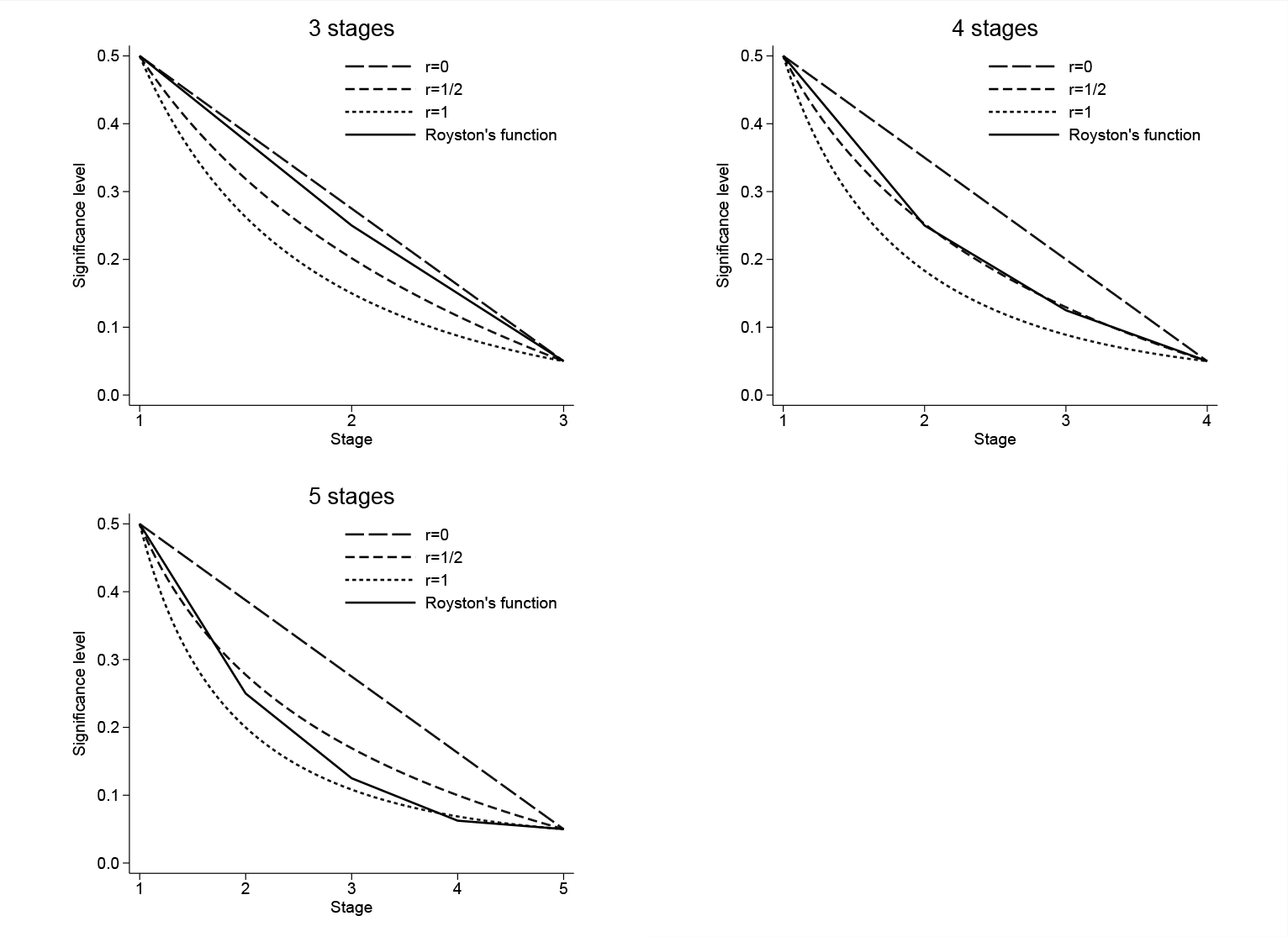
Examples of α functions generated using (3) (“Royston’s function”) and (4) for r = 0, 0.5, and 1; J = 3, 4, and 5 stages; α ₁ = 0.5; and α_J = 0.05.

Table 1.

Stagewise significance levels obtained from the α functions shown in figure 1 for three-, four-, and five-stage designs

Number of stages, J	Stage	0	r in (4) 0.5	1	Royston’s function (3)
3	1	0.50	0.50	0.50	0.50
	2	0.28	0.20	0.15	0.25
	3	0.05	0.05	0.05	0.05
4	1	0.50	0.50	0.50	0.50
	2	0.35	0.25	0.18	0.25
	3	0.20	0.13	0.09	0.13
	4	0.05	0.05	0.05	0.05
5	1	0.50	0.50	0.50	0.50
	2	0.39	0.28	0.20	0.25
	3	0.28	0.17	0.11	0.13
	4	0.16	0.10	0.07	0.06
	5	0.05	0.05	0.05	0.05

Figure 1 shows that as r increases, the α functions in (4) become more curved. This causes the significance level to decrease more rapidly during the initial stages, thus increasing their sample size and duration (except for the first stage, whose duration is determined by the fixed value α ₁). The functions then level off, so the number of patients recruited in the later stages will decrease. From table 1, it appears that using a value of r greater than 1 for many stages (for example, J = 5) will result in negligibly small decrements in the significance levels between later stages, thus making them too small. On the other hand, α functions that curve in the opposite direction will have very short early intermediate stages, while later stages will be lengthy. Such designs are likely to be impractical and inefficient in practice. Thus, only values of r between 0 and 1 are considered (Bratton 2015). Table 1 also shows that for three or four stages, the significance levels found using (3) almost coincide with a set found using (4). In the five-stage example, the decrease in the significance level between the penultimate (α ₄ = 0.06) and final stages (α ₅ = 0.05) using Royston’s function is too small and unlikely to result in a practical design. The search procedure uses the same (high) power in all intermediate stages and a different lower power at the final stage.

The nstagebinopt command uses the α function in (4) to search for admissible designs and finds the corresponding stagewise design significance levels (α_j ) and power (ω_j ). The command works by first finding a set of feasible designs for a given number of stages and overall operating characteristics and then outputs the admissible designs from this set for all q ∊ [0, 1]. The syntax and output of the command are presented in the following sections, including those applied to the ROSSINI 2 trial design.

3 The nstagebin command

The syntax for nstagebin is described below along with its dialog boxes for simplifying its use, particularly for first-time users.

3.1 Syntax

nstagebin, nstage( # ) accrate( numlist ) alpha( numlist ) power( numlist ) arms( numlist ) theta0( # [#] ) theta1( # [#]) ctrlp( # [#] ) [ ppvc( # ) ppve( # ) aratio( # ) fu( # [#] ) extrat( # ) ltfu( # [#] ) tunit( # ) probs ess nofwer reps( # ) seed( # )]

Note that the number of values given in each numlist must equal the number of stages in the trial as specified in the nstage() option. The options for nstagebin are as follows:

3.2 Options

nstage( # ) specifies the number of trial stages, J. nstage() is required.

accrate( numlist ) specifies the overall anticipated constant accrual rate, r_j , per unit of trial time (see tunit()) in each stage. accrate() is required.

alpha( numlist ) specifies the one-sided significance level, α_j , for each pairwise comparison at each stage, j. Significance levels should decrease with each stage. alpha() is required.

power( numlist ) specifies the nominal power, ω_j , for each pairwise comparison at each stage under the effect specified in theta1(). power() is required.

arms( numlist ) specifies the maximum number of arms actively recruiting in each stage (including the control arm). This option does not necessarily specify the number of arms that will be in each stage by design (except in the first stage). In practice, the actual number of arms that will recruit after the first stage will be determined after deciding whether to stop some arms. Therefore, the number in each stage cannot exceed the number in the previous stage because arms can only be dropped. Smaller numbers of arms can be specified after the first stage to explore the impact on sample size and study length for particular scenarios. arms() is required.

theta0( # [#] ) specifies the absolute risk difference under the null hypothesis, H ₀, for the I and D outcomes, respectively. Typically, these values are both 0 (no difference). If I = D, only one value needs specifying. theta0() is required.

theta1( # [#] ) specifies the minimum risk difference targeted under the alternative hypothesis, H ₁, for the I and D outcomes, respectively. If I = D, only one value needs specifying. theta1() is required.

ctrlp( # [#]) specifies the anticipated control arm event rate for the I and D outcome, respectively. If I = D, only one value needs specifying. ctrlp() is required.

ppvc( # ) specifies the PPV for the control arm, that is, the probability of a patient experiencing the D outcome given he or she has also experienced the I outcome, P (D = 1|I = 1). If I = D, this option does not need specifying.

ppve( # ) specifies the PPV for the experimental arm under the alternative hypothesis. If I = D, this option does not need specifying.

aratio( # ) specifies the allocation ratio, A (number of patients allocated to each experimental arm for each patient allocated to control). For example, aratio(0.5) specifies that one patient is allocated to each experimental arm for every two patients allocated to control. The default is aratio(1) (equal allocation to all arms).

fu( # [#] ) specifies the length of follow-up period from an individual’s randomization to his or her outcome measurement in units of trial time (see tunit()) for the I and D outcomes, respectively. The follow-up period on D should be at least as long as that for I. If I = D, only one value needs specifying. The default is fu(0) (I and D outcomes both observed immediately after randomization).

extrat( # )specifies the delay in units of trial time (see tunit()) between observing the final required outcome for an analysis and the beginning of the next stage. This delay incorporates time for data cleaning, analysis, and the various committee meetings that are usually required. The default is extrat(0) (no delay).

ltfu( # [#]) specifies the loss to follow-up proportion for the I and D outcomes, respectively. This is typically larger for D than I. If I = D, only one value needs specifying. Note that sample sizes are inflated to account for the level of attrition that is expected. The default is ltfu(0) (no loss to follow-up for either outcome).

tunit( # ) defines the code for units of trial time. The codes are 1 = one year, 2 = six months, 3 = one quarter (three months), 4 = one month, 5 = one week, 6 = one day, and 7 = unspecified. tunit() has no influence on the computations and is for information only. The default is tunit(1) (one year).

probs reports the probabilities of the number of arms passing each stage of the study under the global null (H ₀ true for all arms) and global alternative (H ₁ true for all arms) hypotheses.

ess reports the expected sample size of the trial (average number of patients recruited to the trial before it is terminated) under the global null and alternative hypotheses.

nofwer suppresses the calculation of the maximum familywise error rate of the trial (probability of making at least one type I error at the end of the trial under any parameter configuration). In two-arm designs, the FWER is not calculated by default.

reps( # ) specifies the number of replications used in the simulation to calculate the FWER. The default is reps(250000) replicates.

seed( # ) specifies the initial value of the random-number seed used in the simulation to calculate the FWER, which is reproducible.

3.3 Dialog box

The nstagebin command is accompanied with a dialog box to simplify the way in which design parameters can be entered into the command. Once installed, the box can be accessed by typing “db nstagebin” into the Stata command line. The tabs of the dialog box are presented in figures 2–5. Because we would like to illustrate the capabilities of the dialog box for the more complex I ≠ D designs, we used the design parameters of the example trial presented in appendix A in all the screenshots—for its output, see appendix A.

Figure 2.

Screenshot of the first tab of the nstagebin dialog box: general trial design parameters

Figure 3.

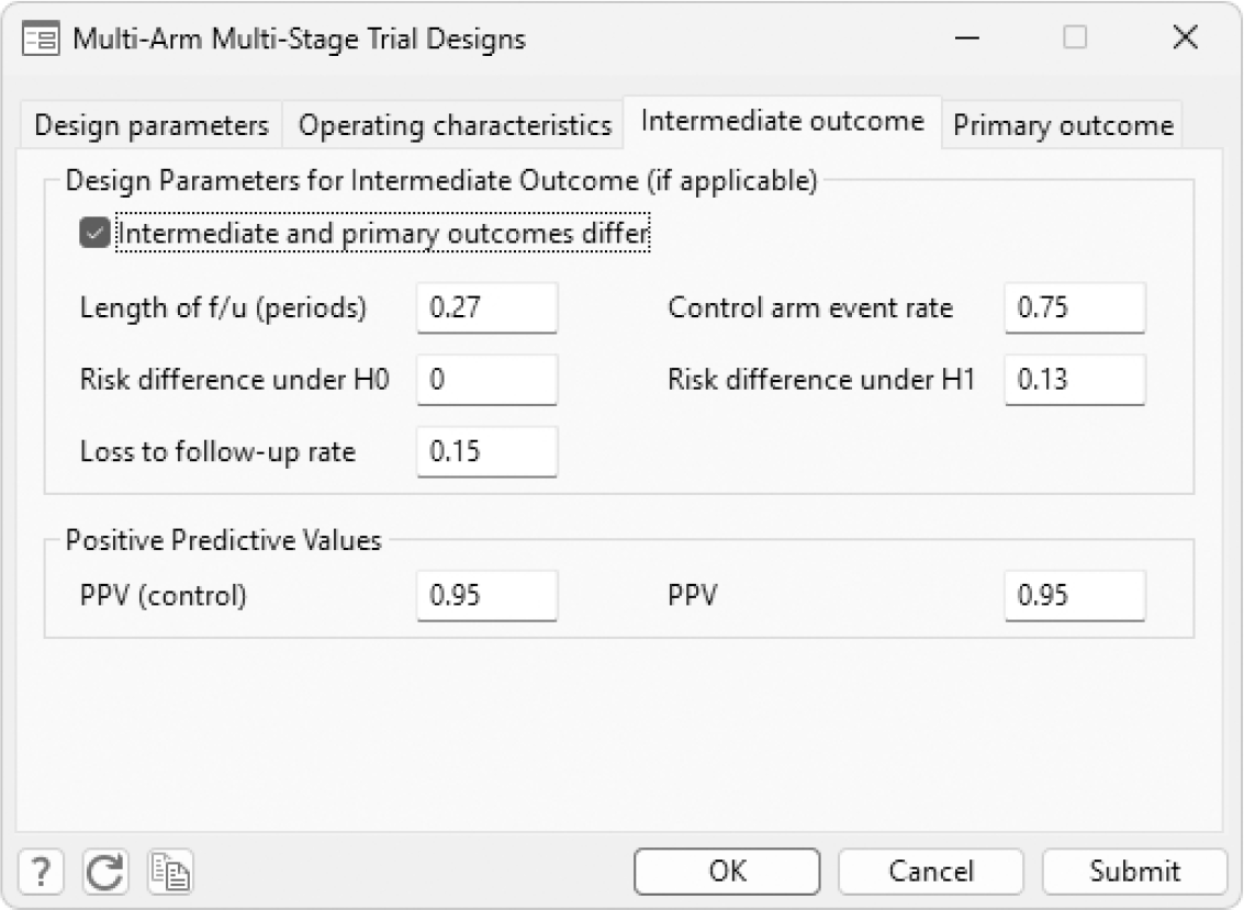
Screenshot of the second tab of the nstagebin dialog box: stagewise operating characteristics

Figure 4.

Screenshot of the third tab of the nstagebin dialog box: parameters for the intermediate outcome (if applicable)

Figure 5.

Screenshot of the final tab of the nstagebin dialog box: parameters for the primary outcome

In the first tab (Design parameters—figure 2), the number of stages, allocation ratio, trial time units, and delay required for interim analyses are entered. In the second tab (Operating characteristics—figure 3), the significance levels, powers, accrual rates, and number of recruiting arms are chosen for each stage of the trial. In the third tab (Intermediate outcome—figure 4), the design parameters for the intermediate outcome (if it differs from the primary outcome) are entered. These include the control event rate, risk differences under H ₀ and H ₁, length of follow-up, and loss to follow-up rate. On the final tab (Primary outcome—figure 5), the analogous parameters are entered for the definitive outcome. Also on the third tab, the PPVs of I on D are entered for the control and experimental arms.

4 The nstagebinopt command

The syntax for nstagebinopt is presented in the following subsections.

4.1 Syntax

nstagebinopt, nstage( # ) arms( # ) alpha( # ) power( # ) theta0( # [#]) theta1( # [#]) ctrlp( # [#]) aratio( numlist ) [ppv( # ) save( string ) fwer pi( # ) p( numlist ) ltfu( # [#]) fu( # ) accrate( numlist ) acc( # ) plot]

4.2 Options

nstage( # ) specifies the number of trial stages, J. nstage() is required.

arms( # ) specifies the number of arms at the start of the study (including control arm), K + 1. arms() is required.

alpha( # ) specifies the desired overall one-sided type I error rate of each pairwise comparison in the trial. If the fwer option is specified, the value specified in alpha() is the desired familywise error rate of the study. alpha() is required.

power( # ) specifies the overall pairwise power. power() is required.

theta0( # [#]) specifies the absolute risk difference under the null hypothesis, H ₀, for the I and D outcomes. Typically, these values are both 0. If I and D are the same, then only one value needs specifying. theta0() is required.

theta1( # [#]) specifies the minimum risk difference targeted under the alternative hypothesis, H ₁, for the I and D outcomes. Typically, either these values are equal or the target difference is smaller for the D outcome. If I and D are the same, then only one value needs specifying. theta1() is required.

ctrlp( # [#]) specifies the anticipated control-arm event rate for the I and D outcomes, respectively. If I = D, only one value needs specifying. ctrlp() is required.

aratio( numlist ) specifies the allocation ratios (number of patients allocated to each experimental arm per control-arm patient) that are to be considered in the search procedure for admissible designs. Allocation ratios such as 1 (equal allocation to all arms) or 0.5 (1 patient allocated to each experimental arm for every 2 patients allocated to control) are often used. Note that allocating a higher proportion of patients to control can decrease sample-size requirements if evaluating more than one experimental arm. aratio() is required.

ppv( # ) specifies PPV P (D = 1|I = 1), assumed to be the same in all arms (only needs specifying if I ≠ D).

save( string ) specifies a filename in which to save the characteristics of the admissible designs. The file is saved in the working directory.

fwer specifies that the maximum familywise error rate of the trial should be controlled at the level specified in alpha(). The familywise error rate is the probability of making at least one type I error (false positive) at the end of the trial.

pi( # ) specifies the minimum proportion of the maximum control arm sample size that should be recruited during each stage of the study. For instance, if the maximum control arm sample size is 500 and pi(0.1), then at least 50 patients will be recruited to the control arm during each stage. A higher value of # will increase the speed of the search procedure but may result in finding less efficient admissible designs. The default is pi(0.1).

p( numlist ) defines which alpha functions are to be used in the search procedure. The default is p(0 0.25 0.5) if I = D and p(0 0.25 0.5 0.75 1) if I and D differ.

ltfu( # [#])specifies the loss to follow-up rate for the I and D outcomes, respectively. Typically, the loss-to-follow-up rate is larger for the D outcome than the I outcome. If I and D are the same, then only one value needs specifying. The default is ltfu(0) (no loss to follow-up for either outcome).

fu( # ) specifies the length of the follow-up period (in units of time) for the I outcome. The follow-up period on the D outcome should be the same or longer than that on the I outcome. If I and D are the same, then only one value needs specifying. The default is fu(0) (no follow-up period, that is, outcomes observed immediately after randomization).

accrate( numlist ) specifies the rate per unit of time at which patients enter the trial in each stage of the trial. Accrual rates should be on the same time scale as used for fu(). This option needs specifying only if fu() is specified.

acc( # ) specifies the maximum deviation in overall alpha and power allowed in feasible designs from the desired values. The default is acc(0.0005).

plot produces a plot of the expected sample sizes under H ₀ versus maximum sample sizes of the J-stage admissible designs.

5 Example: Application to the ROSSINI 2 trial

This section presents the outputs from the nstagebinopt and nstagebin commands using the ROSSINI 2 trial as an example.

5.1 ROSSINI 2 MAMS trial

The reduction of SSI using several novel interventions (ROSSINI 2) trial [NCT03838575] is a phase III MAMS design investigating in-theater interventions to reduce SSI. The composite binary outcome of SSI up to 30 days is the definitive outcome that is used at both the interim and the final stages of this trial, that is, I = D MAMS design. In this eight-arm, three-stage MAMS trial, three interventions (skin prep, drape, and sponge) are being tested, with patients being randomized to receive none (control arm), one, or any combination of these interventions; that is, there are seven experimental arms in total. The primary outcome measure θ is the absolute difference in the proportion of patients reporting SSI up to 30 days after surgery between each of the experimental arms and that of the control arm. The same primary outcome measure is used at all stages for analysis and dropping of arms. No formal stopping rule for early evidence of efficacy has been specified at the design stage of the trial. The trial design also allowed for treatment selection. For simplicity, we disregard this aspect of the trial design and consider it as a standard MAMS trial. Table 2 shows the stagewise design parameters for the ROSSINI 2 trial.

Table 2.

Design specification for the eight-arm three-stage ROSSINI 2 MAMS trial. The target effect size is 5% reduction in the SSI event rate in each of the seven experimental arms from the control-arm event rate of 15%—see section 5.3 for more details.

	Stagewise operating characteristics
Stage	Power	Sig. level	Ctrl. arm patients
1	0.94	0.40	402
2	0.94	0.14	854
3	0.91	0.005	1887
Overall pairwise power	0.85
Overall FWER	0.025

In this trial, the overall FWER was strongly controlled at 0.025 (one-sided) to account for multiplicity as a result of multiple pairwise comparisons. The overall pairwise power is 0.85. The nstagebinopt command used these values to find admissible MAMS designs and determine the corresponding stagewise operating characteristics, α_j and ω_j . Then the nstagebin command calculates the stagewise sample sizes and trial timelines given stagewise (design) operating characteristics that are determined by nstagebinopt, as well as all the other design parameters such as the number of arms and stages and control arm event rate.

5.2 nstagebinopt output

In multiarm trials, nstagebinopt outputs the stagewise operating characteristics and expected sample sizes under the global null and alternative hypotheses, that is, E(N|H ₀) and E(N|H ₁), for each admissible J-stage design that minimizes the loss function in (2) for some q ∊ [0, 1]. The command can also save this information in a dataset if you specify the save() option and can produce a plot of E(N|H ₀) versus E(N|H ₁) by choosing the plot option—see figure 6. Each admissible design can then be entered into the nstagebin command to explore them in more detail—see section 5.3 for the code and its output, that is, stage durations and sample sizes.

In the design stage of the ROSSINI 2 trial, the control-arm SSI rate was assumed to be 0.15, that is, specified using the ctrlp(0.15) option in both commands. The trial is powered to detect a target SSI rate of 0.10 in each of the experimental arms, an absolute reduction of θ = 5% (theta1(-0.05)) and a relative reduction of 33.3%. Patients are allocated to the control arm with a 2:1 ratio (aratio(0.5)) to increase power for each of the pairwise comparisons. In stage 1, which includes the pilot phase, the accrual rate was (on average) assumed to be 118 patients per month. This was expected to increase to 248 patients per month in the subsequent stages (accrate(118 248 248)). These recruitment targets were achievable based on the experience with the previous ROSSINI-1 trial. Further, it was assumed that 4% of patients will be lost to follow-up (ltfu(0.04)) or that the primary outcome evaluation will be missing, for example, surgery not done. For the interim-stage analyses, once the target number of patients is recruited, it was expected that around 4 months will pass until the decision time regarding stopping or continuing research arms, that is, fu(4). This was to allow for 30-day follow-up, captured data to be entered, interim analysis to be performed, and Independent Data Monitoring Committee and Trial Steering Committee meetings to be held.

The output from the nstagebinopt command is shown below for the ROSSINI 2 MAMS trial with the (one-sided) FWER of 0.025, which is alpha(0.025), and the pairwise power of 0.85, which is power(0.85). Note that the FWER is calculated using simulations in both the nstagebin and the nstagebinopt commands. Thus, both commands calculate (and present) the corresponding Monte Carlo error using the formula $\sqrt{{FWER \times (1 - FWER)} / N}$ , where FWER is the calculated overall FWER and N is the number of simulations. The range of values of q (q-range) for which each design minimizes the loss function is also presented. Minimax designs (admissible for q = 1) use a high power in the intermediate stages so that the lowest possible power is chosen in the final stage, thus reducing the maximum sample size—see design number 4 in the output. The stagewise powers in the intermediate and final stages then balance out as q decreases [that is, as E(N|H ₀) becomes more of a factor in choosing a design]. The general pattern observed in the output and figure 6, which plots the expected sample sizes under the global null and alternative hypotheses for the four different admissible designs, is that as the expected sample size of the admissible designs increases under the global alternative hypothesis, E(N|H1), the expected sample size under the global null hypothesis, E(N|H0), decreases. Note that this trend is nonlinear.

The results indicate that the design that is admissible for q ∊ [0.10, 0.65] has an expected sample size of 4,683 patients, which is just 25 patients higher than the nulloptimal design with 4,658 patients. However, this admissible design has a much smaller E(N|H ₁) than that of the null optimal design. Overall, this design is the preferred choice. So the chosen stagewise significance levels and powers are used in the nstagebin command for sample-size calculations.

Figure 6.

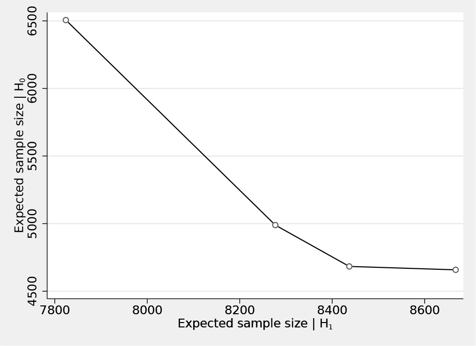
The expected sample sizes for the four different admissible designs presented in section 5.2—see nstagebinopt output

5.3 nstagebin output

This section presents the nstagebin command to calculate the required sample size for the ROSSINI 2 MAMS design, together with its output. Most of the design parameters have been defined in section 5.2. The chosen design with the corresponding stagewise significance levels and power from the nstagebinopt output are used in the nstagebin command to calculate the stagewise sample sizes and timelines. The selected significance levels are 0.40, 0.14, and 0.005—that is, alpha(0.40 0.14 0.005). Stages 1 and 2 stagewise significance levels, that is, 0.40 and 0.14, act as the interim stopping boundaries for lack of benefit on the p-value scale. The selected design stagewise powers (ω_j ) are 94%, 94%, and 91%, respectively, for each of the three stages in all seven pairwise comparisons—power(0.94 0.94 0.91). These stagewise design parameters ensure an overall (one-sided) FWER of 0.025 and a pairwise power of 0.85.

6 Conclusions

This article presented the nstagebin and nstagebinopt commands to find efficient MAMS designs with binary intermediate and definitive outcomes. The commands (and associated dialog boxes) facilitate sample-size calculations and planning for such complex studies. The target treatment effect in nstagebin is the absolute risk difference in both I = D and I ≠ D designs. In superiority designs, the analysis can be done on the relative scale, using the odds or risk ratios, with no impact on the operating characteristics of the design—see appendix B of the online supplementary material for the results of our simulations to explore the impact of using different analysis methods on the pairwise operating characteristics of the MAMS design. Both commands can be used to design MAMS trials with a target odds ratio by converting the target (log) odds ratio to the corresponding absolute risk difference (that is, given the control-arm event rate) using the available formula—for example, see (1) in appendix B of the online supplementary material.

In NI designs, however, the same analysis method that was assumed at the design stage should be applied. Otherwise, the type I and II error rates might not be controlled at the prespecified levels because changing the analysis scale in NI designs requires redefining the NI margin (Li et al. 2022). Appendix B of the online supplementary material includes an example NI trial design and the corresponding nstagebin code to calculate the sample size in such designs.

There are limitations within the MAMS framework. First, in designs with a binary intermediate outcome, the designs assume the same probability of experiencing the definitive (binary) outcome given they have had the intermediate outcome (PPV) for the control arm and for experimental arms. This is a reasonable assumption to make and is often the case under the null hypothesis. Second, the MAMS framework and the corresponding nstage suite of commands have been developed for settings where both the intermediate and definitive outcomes are of the same type of distributions. One possible extension is to develop the MAMS approach (and the corresponding software) for intermediate and definitive outcomes that are of different types of distributions. For example, in some conditions a continuous (information-rich) marker can sometimes be assessed earlier as an intermediate outcome ahead of the primary binary outcome such as death or response to treatment (Choodari-Oskooei et al. 2023). This broadens the application of MAMS designs to a larger spectrum of health conditions.

Finally, we validated the stagewise sample sizes from nstagebin. We compared the results with those obtained from the artbin Stata command, which can be used only for single-stage designs. The sample-size calculations in both agree across a wide range of design scenarios. The validation script is available in the online supplementary material.

We hope that the commands and this article can facilitate the uptake and implementations of MAMS designs and help to optimize MAMS designs with binary outcomes.

8 Programs and supplemental materials

Supplemental Material, sj-zip-1-stj-10.1177_1536867X231196295 - Facilities for optimizing and designing multiarm multistage (MAMS) randomized controlled trials with binary outcomes

Supplemental Material, sj-zip-1-stj-10.1177_1536867X231196295 for Facilities for optimizing and designing multiarm multistage (MAMS) randomized controlled trials with binary outcomes by Babak Choodari-Oskooei, Daniel J. Bratton and Mahesh K. B. Parmar in The Stata Journal

Footnotes

7 Acknowledgments

We are grateful to Professor Stephen Jenkins, the editor, and an external reviewer for useful comments and suggestions on the earlier draft of this manuscript, which have improved the article markedly. We also thank Professor Ian White for helpful comments on the earlier draft of this manuscript. This work was supported by the Medical Research Council (MRC) grant numbers MC_UU_00004_09 and MC_UU_123023_29.

8 Programs and supplemental materials

To install a snapshot of the corresponding software files as they existed at the time of publication of this article, type

For the latest version of the nstagebin and nstagebinopt commands, type

References

Abery

J. E.

Todd

. 2018. Comparing the MAMS framework with the combination method in multi-arm adaptive trials with binary outcomes. Statistical Methods in Medical Research 28: 1716–1730. https://doi.org/10.1177/0962280218773546.

Barthel

F. M.-S.

Royston

Parmar

M. K. B.

. 2009. A menu-driven facility for sample-size calculation in novel multiarm, multistage randomized controlled trials with a time-to-event outcome. Stata Journal 9: 505–523. https://doi.org/10.1177/1536867X0900900401.

Bratton

D. J.

2015. Design issues and extensions of multi-arm multi-stage clinical trials. PhD thesis, University College London.

Bratton

D. J.

Parmar

M. K. B.

Phillips

P. P. J.

Choodari-Oskooei

. 2016. Type I error rates of multi-arm multi-stage clinical trials: Strong control and impact of intermediate outcomes. Trials 17: 309. https://doi.org/10.1186/s13063-016-1382-5.

Bratton

D. J.

Phillips

P. P. J.

Parmar

M. K. B.

. 2013. A multi-arm multistage clinical trial design for binary outcomes with application to tuberculosis. BMC Medical Research Methodology 13: 139. https://doi.org/10.1186/1471-2288-13-139.

Choodari-Oskooei

Sydes

Royston

Parmar

M. K. B.

. 2022. Multi-arm multi-stage (MAMS) platform randomized clinical trials. In Principles and Practice of Clinical Trials, ed. Piantadosi

Meinert

C. L.

1–36. Cham, Switzerland: Springer. https://doi.org/10.1007/978-3-319-52677-5_110-1.

Choodari-Oskooei

Thwin

S. S.

Blenkinsop

Widmer

Althabe

Parmar

M. K. B.

. 2023. Treatment selection in multi-arm multi-stage designs: With application to a postpartum haemorrhage trial. Clinical Trials 20: 71–80. https://doi.org/10.1177/17407745221136527.

Dunnett

C. W.

1955. A multiple comparison procedure for comparing several treatments with a control. Journal of the American Statistical Association 50: 1096–1121. https://doi.org/10.2307/2281208.

Jung

S.-H.

Lee

Kim

George

S. L.

. 2004. Admissible two-stage designs for phase II cancer clinical trials. Statistics in Medicine 23: 561–569. https://doi.org/10.1002/sim.1600.

10.

Quartagno

Böhringer

van Geloven

. 2022. Choosing and changing the analysis scale in non-inferiority trials with a binary outcome. Clinical Trials 19: 14–29. https://doi.org/10.1177/17407745211053790.

11.

Parmar

M. K. B.

Barthel

F. M.-S.

Sydes

Langley

Kaplan

Eisenhauer

Brady

, et al. 2008. Speeding up the evaluation of new agents in cancer. Journal of the National Cancer Institute 100: 1204–1214. https://doi.org/10.1093/jnci/djn267.

12.

ROSSINI 2. 2023. Reduction of surgical site infection using several novel interventions. https://www.birmingham.ac.uk/research/bctu/trials/coloproctology/rossini-2/index.aspx.

13.

Royston

Barthel

F. M.-S.

Parmar

M. K. B.

Choodari-Oskooei

Isham

. 2011. Designs for clinical trials with time-to-event outcomes based on stopping guidelines for lack of benefit. Trials 12: 81. https://doi.org/10.1186/1745-6215-12-81.

14.

Royston

Parmar

M. K. B.

Qian

. 2003. Novel designs for multi-arm clinical trials with survival outcomes with an application in ovarian cancer. Statistics in Medicine 22: 2239–2256. https://doi.org/10.1002/sim.1430.

15.

Sydes

M. R.

Parmar

M. K. B.

Mason

M. D.

Clarke

N. W.

Amos

Anderson

de Bono

, et al. 2012. Flexible trial design in practice—stopping arms for lack-ofbenefit and adding research arms mid-trial in STAMPEDE: A multi-arm multi-stage randomized controlled trial. Trials 13: 168. https://doi.org/10.1186/1745-6215-13-168.

Supplementary Material

Please find the following supplemental material available below.

For Open Access articles published under a Creative Commons License, all supplemental material carries the same license as the article it is associated with.

For non-Open Access articles published, all supplemental material carries a non-exclusive license, and permission requests for re-use of supplemental material or any part of supplemental material shall be sent directly to the copyright owner as specified in the copyright notice associated with the article.

0.20 MB

0.00 MB