hdps: A suite of commands for applying high-dimensional propensity-score approaches

Abstract

Large healthcare databases are increasingly used for research investigating the effects of medications. However, a key challenge is capturing hard-to-measure concepts (often relating to frailty and disease severity) that can be crucial for successful confounder adjustment. The high-dimensional propensity score has been proposed as a data-driven method to improve confounder adjustment within healthcare databases and was developed in the context of administrative claims databases. We present hdps, a suite of commands implementing this approach in Stata that assesses the prevalence of codes, generates high-dimensional propensity-score covariates, performs variable selection, and provides investigators with graphical tools for inspecting the properties of selected covariates.

1 Introduction

Large healthcare databases, such as electronic health records (EHRs), have become widely used for investigating the benefits and harms of medications (Stürmer et al. 2006). These data have the potential to answer important questions surrounding the long-term and rare effects of medications. However, confounding bias is often a major concern and can result in misleading conclusions being drawn (Brookhart et al. 2010; Freemantle et al. 2013). Confounding bias is the systematic difference between a group of patients receiving treatment and a relevant comparative group (Brookhart et al. 2010). In large healthcare databases, these differences are often due to a complex combination of factors relating to both clinician-prescribing behavior and patient-level variables (for example, surrounding disease severity) (Brookhart et al. 2010). To overcome confounding bias, investigators must identify and appropriately adjust for a set of confounders that sufficiently mitigate confounding bias (Brookhart et al. 2010).

Confounder adjustment is often achieved using outcome regression: modeling the relationship between an outcome variable and a treatment (or exposure) variable conditional on a set of confounders. However, analysis based on the propensity score (PS) is often preferred in the context of large healthcare databases given the ability to summarize a large amount of confounder information in one score (Rosenbaum and Rubin 1983; Jackson, Schmid, and Stuart 2017). PS analysis involves modeling the treatment allocation process using a set of observed variables to estimate the conditional probability of initiating the treatment under investigation. There are several methods (for example, weighting or matching methods) for estimating treatment effects based on the estimated PSs. Williamson et al. (2012) and Austin (2011) provide general introductions to the concepts behind PS analysis. Brookhart et al. (2006) discuss the types of variables to be included in PS models, indicating that all confounders and risk factors should be included. Finally, indications for PS analysis and current practice in pharmacoepidemiology are discussed by Jackson, Schmid, and Stuart (2017).

As with outcome regression models, the key assumption of no unmeasured confounding is required to yield unbiased treatment-effect estimates from PS methods (Williamson et al. 2012). However, in large healthcare databases, successful adjustment for confounding often relies on capturing concepts, such as frailty, that are hard to measure (even in controlled settings, for example, randomized controlled trials) (Schneeweiss et al. 2009).

The high-dimensional propensity-score (HDPS) algorithm has been proposed as an extension to PS methodology, designed to maximize capture of hard-to-measure or otherwise unmeasured concepts in large healthcare databases (Schneeweiss et al. 2009). The HDPS is a semiautomated data-driven approach for generating and selecting potential features (typically codes captured as part of the routine recording of clinical and administrative information) measured prior to treatment initiation that are likely to be informative of disease severity and frailty (Schneeweiss et al. 2009). HDPS approaches aim to optimize confounder control in a given setting by adjusting for several hundred of these data-derived covariates. The benefits of these approaches have been illustrated in many settings, resulting in their popularity as methods for confounder adjustment in pharmacoepidemiological studies (Schneeweiss 2018). Furthermore, while implementations of HDPS exist in SAS and R, these approaches have yet to be formally implemented in Stata (Rassen et al. 2020; Lendle 2017).

We introduce hdps, a suite of commands for performing the HDPS procedure and investigating properties of the selected covariates (Schneeweiss et al. 2009; Wyss et al. 2018a). These commands allow investigators to specify commonly used tuning parameters surrounding key decisions in the HDPS, for example, the method of covariate prioritization and number of covariates selected (Schneeweiss et al. 2009; Patorno et al. 2014; Wyss et al. 2018b). Additionally, recent modifications tailoring the HDPS for use in U.K. EHRs are also implemented (Tazare et al. 2020). We demonstrate how to conduct the HDPS procedure and perform a PS analysis with the selected covariates.

2 HDPS

Information in large healthcare databases is typically stored in the form of discrete codes, of which there can be thousands. Codes capture various aspects of the healthcare system and (while the exact information will vary between databases) will often include information on clinical diagnoses and prescribed medications. In some cases, laboratory test result data and hospital admission and discharge information may also be available (Schneeweiss and Avorn 2005).

The HDPS is a multistep algorithm that transforms codes recorded in a healthcare database into covariates to be included within a PS analysis. The codes considered during the HDPS procedure are recorded prior to treatment initiation to avoid inadvertent adjustment for covariates on the causal pathway from treatment to outcome (Schneeweiss et al. 2009). This assessment window is usually defined during the one year prior to treatment initiation. The steps of the HDPS are summarized as follows (figure 1), and more detailed methodological guidance is available in articles by Rassen et al. (2022) and Tazare et al. (2022):

Data dimensions: Specify the data to be used for deriving data-driven covariates. Typically, this involves separating information in the healthcare database into multiple datasets, capturing different aspects of clinical care or coding information. In U.K. EHRs, we may separate codes pertaining to clinical, referral, hospitalization, and prescription information. While codes can be used directly, investigators may, where possible, exploit hierarchical coding systems to aggregate code information (Le et al. 2013). For example, when using International Classification of Disease 10th edition (ICD10) codes, investigators may group information at the four-digit, three-digit, or chapter granularity level. Le et al. (2013) highlight that aggregation may improve the performance of the HDPS in settings with smaller cohort sizes, rare outcome incidence, or low exposure prevalence.

Prevalence filter: Identify the most prevalent codes in each dimension (typically, 200 are chosen) (Schneeweiss et al. 2009). This step is optional, and instead all codes can be assessed for potential inclusion.

Assess recurrence: For each code identified in the previous step, generate up to three binary covariates based on how frequently patients have a particular code recorded in the aforementioned assessment window:

$\begin{array}{c}\text{ Once }=\{\begin{array}{cc}1& \text{ if code recorded }\ge \text{ once }\\ 0& \text{ otherwise }\end{array} \\ \text{ Sporadic } = \{\begin{array}{cc}1& \text{ if code recorded }\ge \text{ median }\\ 0& \text{ otherwise }\end{array} \\ \text{ Frequent }= \{\begin{array}{cc}1& \text{ if code recorded }\ge \text{ upper quartile }\\ 0& \text{ otherwise }\end{array}\end{array}$

Recent work by Tazare et al. (2020) implementing the HDPS in U.K. EHRs extends the bottom frequency category to capture information recorded “Ever” in a patient’s history. For codes originating from data dimensions where this extra information is used, the “Once” variable is replaced by

$\text{ Ever }=\{\begin{array}{ll}1\hfill & \begin{array}{l}\text{if code recorded anytime in patient’s history} \\ \text{(prior to treatment initiation)}\end{array}\hfill \\ 0\hfill & \text{otherwise }\hfill \end{array}$

Prioritize covariates: Prioritize the set of binary covariates to identify those most important for confounder adjustment.

Bross formula: Typically, this prioritization is performed using the Bross formula to define a multiplicative bias term (Bross 1966; Schneeweiss et al. 2009; Wyss et al. 2018a) as

${\text{Bias}}_{\text{M}}=\frac{{\text{P}}_{\text{C}1}\left({\text{RR}}_{\text{CD}}-1\right)+1}{{\text{P}}_{\text{C}0}\left({\text{RR}}_{\text{CD}}-1\right)+1}$

where RR_CD is the covariate-outcome risk ratio and P_C1 and P_C0 are the prevalence of the covariate in the treated and untreated, respectively. Covariates are ranked in descending order by |log(Bias_M)|, with higher numbers indicating greater potential for contributing to confounding bias.

Exposure based: Rassen et al. (2011) have shown that, in studies of few treated patients or few outcome events, prioritizing covariates based solely on the covariate-exposure relationship can perform well compared with the Bross formula.

Select covariates: From the set of prioritized covariates, a subset is chosen for inclusion in the PS model. This is a key decision in the HDPS procedure, and depending on the setting, results can vary considerably (Patorno et al. 2014; Wyss et al. 2018b). Typically, 200 or 500 covariates are selected (Schneeweiss et al. 2009; Schneeweiss 2018); however, these numbers are arbitrary, and we recommend testing the sensitivity of results to this decision.

Diagnostic tools: In any PS analysis, it is important to assess covariate balance and perform diagnostics (Austin 2009; Granger et al. 2020). For HDPS analyses, it is additionally important to understand the covariates selected by identifying potentially influential covariates and investigating covariate balance (Franklin et al. 2015; Patorno et al. 2014).

PS analysis: The final step is performing a standard PS analysis. The first stage is to estimate the PS, usually via a logistic regression modeling the treatment variable on a set of covariates. In the HDPS setting, this set of covariates includes 1) a set of “investigator” covariates identified based on clinical knowledge and 2) the set of selected HDPS covariates. The second stage involves estimating treatment effects from an outcome model, incorporating the PS using adjustment, matching, weighting, or stratification (Williamson et al. 2012).

Figure 1.

Summary of a generic implementation of the HDPS algorithm, identifying the top 200 most prevalent codes per dimension and selecting the top 500 Bross-ranked HDPS covariates. Steps highlighted in gray represent those implemented in the hdps package. Abbreviations: Dim., dimension.

3 The hdps commands

3.1 Data formats

The hdps suite uses two types of input datasets: a cohort dataset and at least one data dimension.

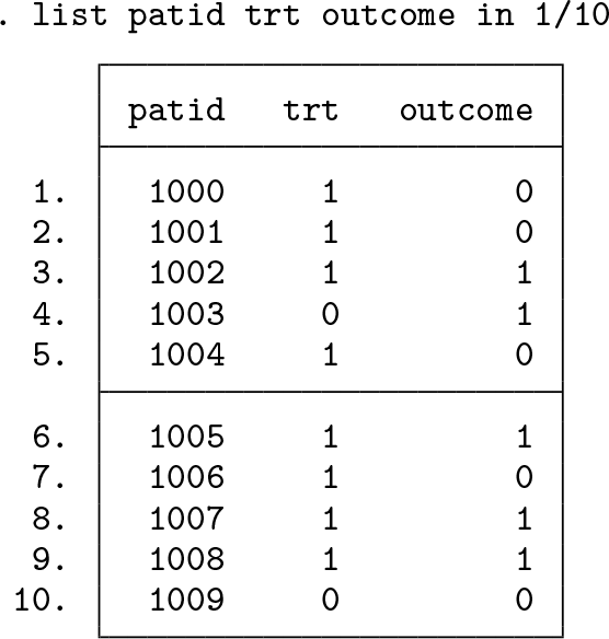
Cohort dataset: One observation per patient that includes at least a patient identifier (stored in all datasets as a string variable), a binary treatment variable, and a binary outcome variable (both stored as numeric variables). We show the first 10 observations from an example dataset below:

Data dimensions: A long-format dataset containing codes recorded during the HDPS assessment window for all patients in the cohort. A separate dataset should be prepared for each data dimension. This dataset will often be many observations per patient per code. We show the first 10 observations for an example patient, highlighting multiple recordings for codes within the assessment window.

Ever dimensions: If “Ever” information (as described in section 2, step 3) is being assessed for a given data dimension, a secondary dataset should be provided. These data will be in long format and contain codes recorded in a patient’s entire history (prior to treatment initiation). Because we want to capture the presence only of a specific code, this dataset should be one observation per patient per code. Note that, to reduce the size of this dataset, users may wish to remove any code already recorded during the assessment window.

3.2 The hdps setup command

The hdps setup command declares the data dimensions and key variables used throughout the HDPS procedure, further specifying the directory for outputted datasets. Set the current directory to a folder containing all necessary data, and load the cohort dataset into memory.

3.2.1 Syntax

hdps setup dimension [dimension…], save( string ) study( string ) patid( varname ) exposure( varname ) outcome( varname )

dimension is specified for each data dimension required, using the following syntax:

( filename , varname [ever])

3.2.2 Dimension syntax

filename specifies the filename for the data dimension.

varname specifies the variable in the data dimension containing codes. Note that this is a required term and must be the first term specified.

ever optionally specifies that the recurrence assessment for the dimension should incorporate “Ever” information. Where ever is specified for a particular dimension, the “Ever” dimension must be named filename _ever, and the variable containing codes must be named varname.

3.2.3 Overall options

save( string ) specifies a directory where output files will be saved. save() is required.

study( string ) specifies a study name that serves as a prefix on all output files. study() is required.

patid( varname ) specifies the variable containing the patient identifiers in the cohort dataset and data dimensions. patid() is required.

exposure( varname ) specifies the binary treatment or exposure variable. exposure() is required.

outcome( varname ) specifies the binary outcome variable. outcome() is required.

3.2.4 Output

A summary is reported displaying the specifications for the declared data dimensions. hdps setup saves a dataset called study _cohort_info.dta containing the patient identifier, treatment, and outcome variables.

3.3 The hdps prevalence command

hdps prevalence performs step 2 of the HDPS algorithm, identifying the most prevalent codes within each data dimension and calculating distribution cutoffs used to assess code recurrence. Additionally, for each patient, the command assesses the total frequency of each selected code. To run hdps prevalence, you must have previously specified data dimensions using hdps setup.

3.3.1 Syntax

hdps prevalence, {top( # )| nofilter}

3.3.2 Options

One of the following options must be specified:

top( # ) specifies the number of codes to be selected from each dimension.

nofilter calculates distribution cutoffs and patient frequencies for all available codes. This follows recommendations by Schuster, Pang, and Platt (2015) suggesting that a prevalence filter can result in the omission of codes important for confounder adjustment, with a low marginal prevalence.

3.3.3 Output

The number of codes successfully selected from each dimension is reported in the Results window. Two datasets are outputted: 1) a summary of the codes selected, reporting the median and upper quartile, used as cutoffs for defining the binary covariates generated (study _feature_prevalence.dta); and 2) the per-patient code totals for each code selected (study _patient_totals.dta).

3.4 The hdps recurrence command

The hdps recurrence command performs step 3 of the HDPS, creating binary covariates based on the cutoffs described in section 2. hdps recurrence requires the two datasets created by the hdps prevalence command. This is presented as a separate command because of the possible computational burden in settings with many dimensions or patients.

3.4.1 Syntax

hdps recurrence

3.4.2 Output

The total number of binary HDPS covariates generated is returned in the Results window. The full set of covariates is outputted in a dataset called study _hdps_covariates.dta.

3.5 The hdps prioritize command

Finally, the hdps prioritize command is used to prioritize and perform variable selection on the set of covariates created by the hdps recurrence command (section 2; steps 4 and 5).

3.5.1 Syntax

hdps prioritize, method( string ) top( numlist ) [zerocell]

3.5.2 Options

method( string ) specifies the method of covariate prioritization. Available methods are bross or exposure, as outlined in section 2. method() is required.

top( numlist ) specifies the number of covariates to be selected. To obtain multiple datasets varying the number of covariates selected, you can provide a list of integers, for example, top(200 500). top() is required.

zerocell applies a correction of 0.1 to cells used in the calculation of the Bross. As described by Rassen et al. (2011), covariates cannot be considered for inclusion if the components of the Bross formula are undefined or equal to 0. In settings with few outcomes, this is particularly likely to affect RR_CD. Applying this correction therefore allows computation of these values and for covariates to remain under consideration.

3.5.3 Output

The hdps prioritize command outputs a dataset containing the data used to calculate the ranking information for each of the HDPS covariates (study _bias_info.dta). Additionally, a dataset containing the selected number of covariates (k) for each scenario specified in the top() option is outputted in the form study _hdps_covariates_top_k.dta.

3.6 The hdps graphics command

The hdps graphics command is a stand-alone command for graphically assessing the properties of covariates generated and selected by the HDPS procedure. There are three graphical diagnostic tools available (illustrated in section 4).

Bross inspects the distribution of ranked Bross values used for covariate prioritization (Patorno et al. 2014). This plot requires specifying variables containing the bias ranking values and the numerical rank of covariates (abs_log_bias and rank; the variables are available in study _bias_info.dta).

Prevalence investigates covariate balance by comparing the prevalence in the two treatment groups (Franklin et al. 2015). This plot requires specifying variables containing these two prevalences (pc1 and pc0; the variables are available in study _bias_info.dta).

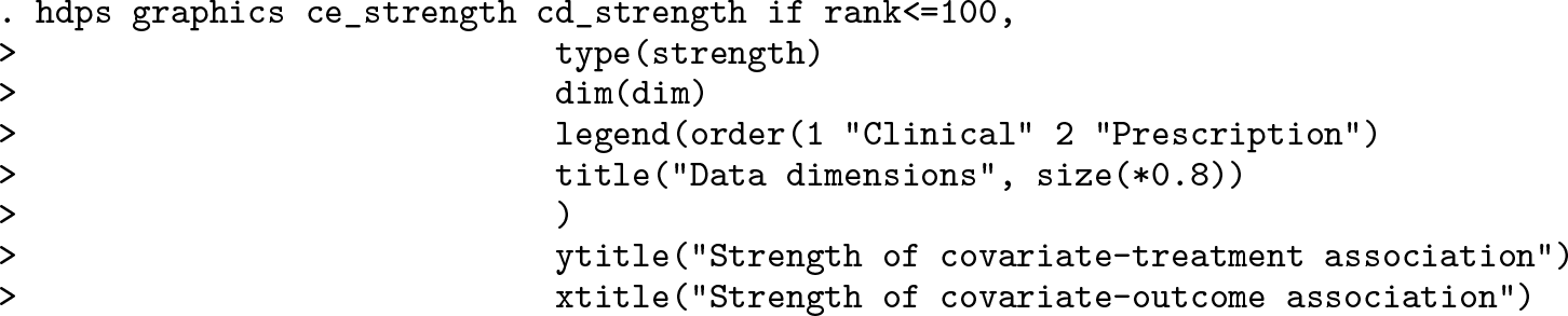
Strength compares the relationship between covariate-exposure (ce_strength) and covariate-outcome (cd_strength) associations; the variables are available in study _bias_info.dta.

3.6.1 Syntax

hdps graphics varlist [if] , type( string ) [ dimension( varname ) pr( # ) graph_options]

where varlist corresponds to variables required by a specific plot type, as described above.

3.6.2 Options

type( string ) specifies one of three plot types: bross, prevalence, or strength (described above). Only one type can be specified at a time. type() is required.

dimension( varname ) specifies a numeric variable identifying the dimension a covariate is derived from. Note that this option is required only for type(prevalence) and type(strength).

pr( # ) specifies a prevalence ratio. The prevalence ratio and its reciprocal will be plotted as dashed lines. The default is to plot prevalence ratios of 2 and 0.5. Note that pr() is an option only for type(prevalence).

graph_options are any of the options documented in [G-3] twoway_options .

3.7 Stored results

The hdps suite stores the following results to e() throughout the HDPS procedure (excluding graphics commands):

4 Example using simulated data

4.1 Simulated data

To illustrate the hdps suite, we use a simulated cohort study design, representative of pharmacoepidemiological studies that use HDPS approaches (summarized in figure 2).

Figure 2.

Example cohort study illustrating the setting in which the HDPS algorithm is traditionally applied

We have simulated a cohort dataset containing a patient identifier (patid), a binary treatment variable (trt: 1 “Study Drug” 0 “Comparator Drug”), a binary outcome variable (outcome: 1 “Yes” 0 “No”), and a set of nine confounders to mimic a priori investigator identified variables. Additionally, two HDPS data dimensions were simulated capturing clinical (ICD-10 codes) and prescription (British National Formularly codes) features based on marginal prevalences observed in a previous study applying HDPS in U.K. EHRs (Tazare et al. 2020). For the clinical data dimension, we have simulated an “Ever” dimension capturing whether an individual has a record for a particular code in his or her entire history (that is, irrespective of whether it occurs in the HDPS covariate assessment window).

These simulated datasets do not attempt to fully capture the complexity of a specific data source. Instead, they have been designed to illustrate the commands and expected data structures. For illustrative purposes, these data have been simulated so that confounding bias will be removed only after inclusion of several data-derived HDPS covariates that would be omitted in a standard analysis. Therefore, we expect the treatment effect to move toward the null after adjustment for the HDPS covariates.

Throughout the following tutorial, we focus on an HDPS analysis with the following tuning parameters: 1) a prevalence filter selecting the top 100 features from each dimension, 2) prioritization using the Bross formula, and 3) selection of the top 100 covariates for inclusion in the PS model.

4.2 HDPS procedure

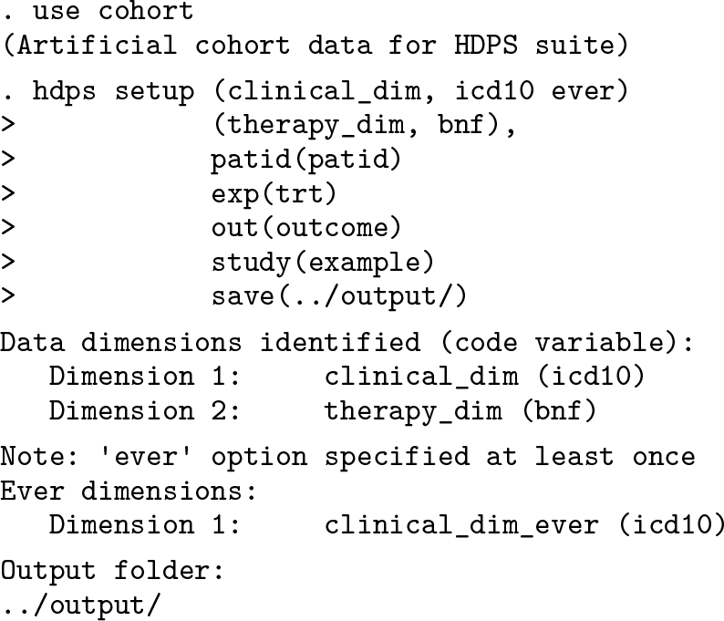
First, ensure that the current working directory includes the cohort dataset and relevant data dimensions. Load the cohort dataset containing the outcome, trt, and patid variables required for the HDPS procedure. We use the hdps setup command to declare these variables and the two data dimensions, specifying the ever option for the clinical dimension.

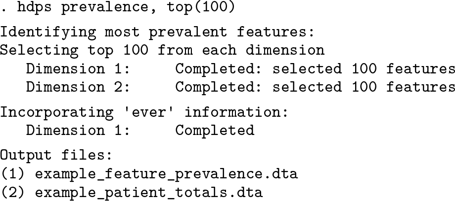
Next, we use the hdps prevalence command to identify the top 100 most prevalent features from each of the data dimensions. Note that we successfully select 100 features from each dimension.

We then run the hdps recurrence command, which assesses the frequency of patient feature recording to define as many as three binary covariates for each feature, using the cutoffs previously described. Note that the 200 features identified using hdps prevalence results in 600 binary HDPS covariates.

Next, we use the hdps prioritize command to select the most important covariates for confounder adjustment. In this instance, we create two datasets containing the top 50 and top 100 covariates based on the Bross formula. While the primary analysis focuses on the model selecting 100 covariates, this shows how easily we can obtain multiple datasets for testing the sensitivity of our results to the number of covariates chosen.

We can now use the hdps graphics command to investigate the properties of the covariates generated and selected.

Having loaded example_bias_info.dta, we first investigate the distribution of ranking scores used to prioritize the covariates. This can be achieved by specifying the bross option and providing the ranking score variable and rank number variable, as below. We note from figure 3 that there are several high-ranking covariates with relatively larger ranking scores, indicating the possible importance for confounder adjustment.

Figure 3.

Distribution of absolute log Bross bias values for each of the top 100 HDPS covariates

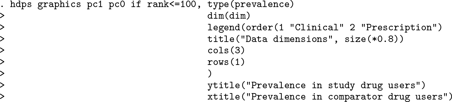
Next, we investigate covariate balance by plotting covariate prevalence in the study drug and comparator drug groups (Franklin et al. 2015). Figure 4 shows similar prevalence in the two groups while also highlighting which dimension covariates were derived from. The dashed lines represent prevalence ratios of 2 and 0.5 to visually highlight covariates with large imbalances between the treatment groups.

Figure 4.

Prevalence of the top 100 HDPS covariates by treatment group. The diagonal line indicates equal prevalence in both groups, and the dashed lines show prevalence ratios of 0.5 and 2.0. The different symbols highlight which dimension the covariate was derived from.

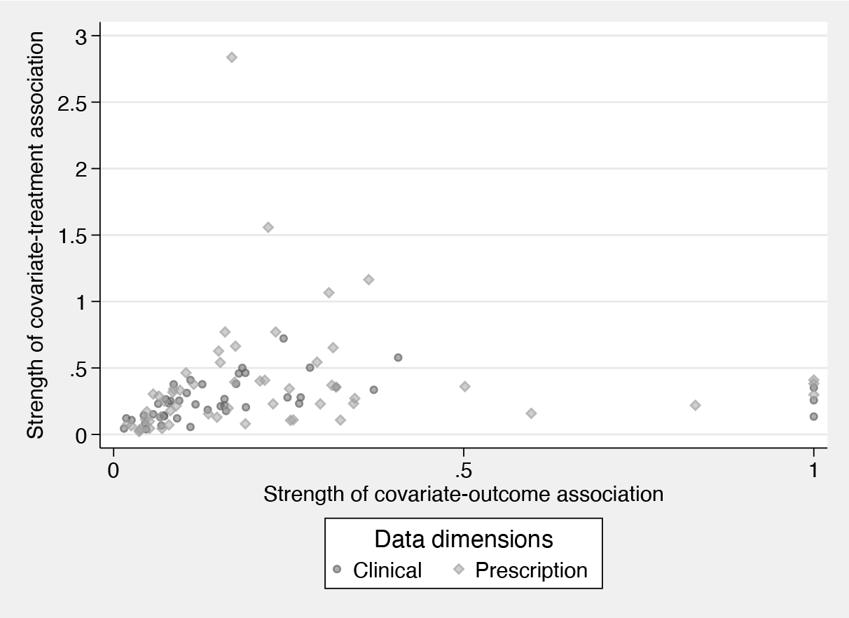
Finally, we inspect the relationship between the strength of covariate-exposure and covariate-outcome associations. In PS analysis, the inclusion of covariates strongly related to the treatment but unrelated to the outcome are known to increase variance Brookhart et al. (2006). Figure 5 can help indicate variables that empirically have these characteristics. Investigators may wish to perform sensitivity analyses assessing the impact of including these variables on the resulting treatment effects and confidence intervals.

Figure 5.

Comparison of the covariate-exposure and covariate-outcome associations for the top 100 Bross-ranked HDPS covariates. The different symbols highlight which dimension the covariate was derived from.

4.3 Investigator PS analysis

In the HDPS literature, investigators often first perform a PS analysis using only the set of covariates identified by the investigators. This provides a useful baseline to compare the performance of subsequent models incorporating the HDPS covariates.

We begin by loading the cohort dataset and describing the variables.

To estimate the PS, we fit a logistic regression, modeling the treatment variable on the set of nine confounders. While other methods such as matching and stratification are available, we focus on incorporating the PS using inverse probability of treatment weights, which are generated below (Austin 2011; Williamson and Forbes 2014).

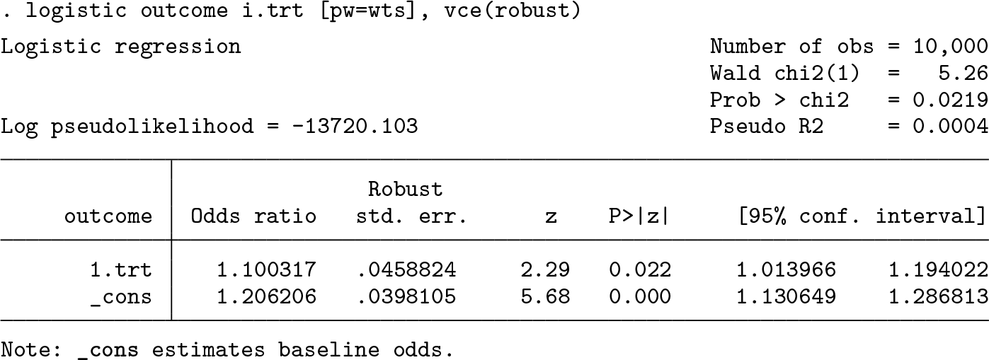
Next we use a weighted logistic regression model to estimate the treatment odds ratio (OR). We apply robust standard errors to acknowledge the lack of independence in the weighted population (Hernán, Brumback, and Robins 2000). However, note that the variance should theoretically account for the estimation of the PS. Our models do not account for this, so the confidence intervals will be slightly conservative (Williamson et al. 2012; Williamson, Forbes, and White 2014).

While we have focused on a binary outcome, these methods can similarly be applied for a time-to-event outcome. The binary outcome indicator would be used throughout the HDPS procedure to select the HDPS covariates. In the PS analysis, the outcome model would be the appropriate survival model.

For the investigator analysis, we obtain some evidence supporting an increased risk of the outcome in those receiving the study drug compared with those receiving the comparator drug (OR 1.10; 95% confidence interval: [1.01 to 1.19]).

4.4 HDPS analysis

We now illustrate how to incorporate the selected HDPS covariates into a PS analysis.

Ensure the cohort dataset is still loaded into memory. The first step is to either drop or rename the previous pscore and wts variables because we will now reestimate the PS. We need to merge the generated set of 100 HDPS covariates to the cohort dataset using the patient identifier (patid). As before, we fit a logistic regression model to estimate the PS and now additionally include the HDPS covariates in this model (the prefixes d1 and d2 represent covariates derived from the clinical and prescription dimensions, respectively). For brevity, we suppress the output from the logistic regression model containing 109 covariates. However, it is important to inspect large models, especially in small samples, where covariates might perfectly predict treatment allocation. Furthermore, note that when you adjust for several hundred HDPS covariates, it may be necessary to increase the maximum matrix size in Stata; for more details, see help matsize.

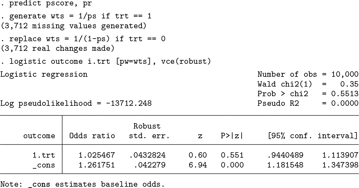
We now estimate the PS and generate new inverse probability of treatment weights before estimating the treatment effect using a weighted logistic regression model.

For the HDPS analysis, we observe that the inclusion of the HDPS covariates has led to a result closer to the expected null association (OR 1.03; 95% confidence interval: [0.94 to 1.11]).

As previously mentioned, the number of covariates selected is a key decision in the HDPS procedure, and we recommend testing the sensitivity of results to this decision. The analysis outlined above can easily be repeated for a different set of covariates by updating the merge file.

5 Conclusions

In this article, we have introduced the hdps suite of commands for applying the HDPS algorithm in Stata. This suite consists of five commands for generating, prioritizing, and visualizing the properties of HDPS covariates. We have illustrated these commands using simulated data and demonstrated how to incorporate the resulting HDPS covariates within a PS analysis.

For illustrative purposes, the analysis presented is based on data simulated with a relatively simple structure. In practice, there will be complex relationships between the codes identified, and investigators will often specify many more data dimensions. The plasmode framework has become a popular method for simulating data more reflective of large healthcare databases and is often used to evaluate the performance of methods in this setting (Franklin et al. 2014).

The main benefit of HDPS methods is seen in settings where information recorded within the healthcare database is likely to be strongly correlated to key confounders that are hard to measure. However, in settings with a well-established or basic confounding structure, the HDPS is not likely to outperform traditional PS or outcome regression methods. Furthermore, it is important to acknowledge that unmeasured confounding may remain an issue even after adjustment for HDPS covariates.

Methodological work surrounding HDPS methods continues to develop rapidly, and any new features in the hdps suite will aim to reflect best practices as they become apparent. A recent review by Schneeweiss (2018) summarizes key areas of development. One topic of growing interest surrounds the possible benefits of combining HDPS and machine learning approaches (Tian, Schuemie, and Suchard 2018; Franklin et al. 2015; Karim, Pang, and Platt 2018; Schneeweiss et al. 2017). For example, in other highdimensional data contexts, machine learning techniques have performed well at selecting important variables compared with conventional methods (Belloni, Chernozhukov, and Hansen 2014).

The hdps suite will be updated and developed, and we would welcome suggestions for improvements and new features. We are also interested in how the data management commands presented might be used to create data-driven covariates in alternative contexts, for example, prediction modeling (Franklin et al. 2016).

7 Programs and supplemental materials

Supplemental Material, sj-zip-1-stj-10.1177_1536867X231196288 - hdps: A suite of commands for applying high-dimensional propensity-score approaches

Supplemental Material, sj-zip-1-stj-10.1177_1536867X231196288 for hdps: A suite of commands for applying high-dimensional propensity-score approaches by John Tazare, Liam Smeeth, Stephen J. W. Evans, Ian J. Douglas and Elizabeth J. Williamson in The Stata Journal