Propensity score matching and complex surveys

Abstract

Researchers are increasingly using complex population-based sample surveys to estimate the effects of treatments, exposures and interventions. In such analyses, statistical methods are essential to minimize the effect of confounding due to measured covariates, as treated subjects frequently differ from control subjects. Methods based on the propensity score are increasingly popular. Minimal research has been conducted on how to implement propensity score matching when using data from complex sample surveys. We used Monte Carlo simulations to examine two critical issues when implementing propensity score matching with such data. First, we examined how the propensity score model should be formulated. We considered three different formulations depending on whether or not a weighted regression model was used to estimate the propensity score and whether or not the survey weights were included in the propensity score model as an additional covariate. Second, we examined whether matched control subjects should retain their natural survey weight or whether they should inherit the survey weight of the treated subject to which they were matched. Our results were inconclusive with respect to which method of estimating the propensity score model was preferable. In general, greater balance in measured baseline covariates and decreased bias was observed when natural retained weights were used compared to when inherited weights were used. We also demonstrated that bootstrap-based methods performed well for estimating the variance of treatment effects when outcomes are binary. We illustrated the application of our methods by using the Canadian Community Health Survey to estimate the effect of educational attainment on lifetime prevalence of mood or anxiety disorders.

1 Introduction

Observational data are increasingly being used to estimate the effects of treatments, exposures and interventions. Advantages to the use of these data include decreased costs compared to the use of randomized experiments, estimates that may be more generalizable since the settings may be more reflective of how the treatment is applied in practice, and the ability to study exposures or interventions to which it would be unethical to randomly assign subjects. The primary disadvantage to the use of observational data is the presence of confounding, which occurs when there are systematic differences in baseline characteristics between treated and control subjects. Due to confounding, differences in outcomes between treatment groups may not be attributable to the treatment, but may reflect systematic differences in subject characteristics between treatment groups.

Statistical methods serve an essential role in observational studies in order to obtain an unbiased estimate of the effect of treatment. An important class of statistical methods comprises those that are based on the propensity score.^1,2 The propensity score is the probability of treatment selection conditional on observed baseline covariates. There are four primary ways in which the propensity score is used: matching on the propensity score, inverse probability of treatment weighting using the propensity score, stratification on the propensity score, and covariate adjustment using the propensity score.^1–3

Health researchers are increasingly using observational data collected using complex survey methods. Complex survey designs include cluster sampling and stratified cluster sampling. ⁴ Examples of such surveys include the National Health and Nutrition Examination Survey conducted by the US Centers for Disease Control and Prevention, the Canadian Community Health Survey (CCHS) conducted by Statistics Canada, and the Health Survey for England conducted by NatCen Social Research on behalf of the Health and Social Care Information Centre. These surveys are intended to provide nationally representative estimates of health status and health behaviors of the population. These surveys are increasingly being used by health researchers to estimate the effect of health behaviors and characteristics.

Complex surveys such as those described previously frequently employ a stratified cluster sampling technique. In such designs, the target population is divided into mutually exclusive strata. These can represent geographical regions of the country if the survey is intended to be nationally representative. Each stratum is divided into clusters. These may represent municipalities or other smaller geographic regions. From each stratum, a random sample of clusters is selected, and from each selected cluster, a random sample of subjects is drawn. A sampling weight is associated with each sampled subject. This sampling weight denotes the number of subjects in the target population who are represented by the sampled subject. Population estimates of statistics require the incorporation of the sampling weights into the analyses. The estimation of standard errors and confidence intervals requires accounting for the sampling design, as it is inappropriate to treat the sample as being a simple random sample.

Given the popularity of propensity score methods and the increasing use of complex surveys for health research, it is somewhat surprising that there is limited methodological work on how to employ propensity score methods in conjunction with complex sample surveys. The objective of the current study was to examine the relative performance of different methods for implementing propensity score matching when using a stratified cluster sample. The paper is structured as follows. In Section 2, we review the brief literature on the use of propensity score methods with complex sample surveys. We highlight issues around the use of propensity score matching that have been neglected in prior studies. In Section 3, we describe an extensive series of Monte Carlo simulations to examine the performance of different methods for implementing propensity score matching with stratified cluster samples. The results of these simulations are reported in Section 4. A case study illustrating the application of these methods is provided in Section 5. In Section 6, we summarize our findings and place them in the context of the existing literature.

2 Propensity score methods and sample surveys

2.1 Review of the existing literature

To the best of our knowledge, only three previous papers have addressed methodological issues around the use of propensity score methods with sample surveys. The first paper, by Zanutto, restricted its focus to the use of stratification on the propensity score and was primarily structured around an empirical analysis. ⁵ She suggested that estimation of the propensity score model not incorporate the sample survey weights, since one is primarily interested in stratifying subjects in the analytic sample, and not in making inferences about the population-level propensity score model. However, she stated that stratum-specific estimates of the effect of treatment should incorporate the survey weights. Thus, she suggested that one incorporate the sampling weights when estimating the effect of treatment, but not when estimating the propensity score model.

In the second paper, DuGoff et al. used a limited set of Monte Carlo simulations to examine the performance of different methods for using the propensity score with survey data. ⁶ They echoed Zanutto’s recommendation that a weighted regression model need not be fit when estimating the propensity score. However, they recommended that the survey weights be included as a covariate in the propensity score model. They considered matching on the propensity score, stratification on the propensity score, and propensity score weighting.

In the third paper, Ridgeway et al. restricted their attention to the use of propensity score weighting with sample surveys. ⁷ They disagreed with the suggestion of the two previous sets of authors that estimation of the propensity score model should not incorporate the sampling weights. They provided a justification for the use of a weighted regression model to estimate the propensity score and used Monte Carlo simulations to compare the performance of four different methods for estimating the propensity score: (i) an unweighted logistic regression model containing baseline covariates; (ii) a weighted logistic regression model containing baseline covariates; (iii) an unweighted logistic regression model containing baseline covariates and the sampling weights as an additional covariate; (iv) a weighted logistic regression model containing baseline covariates and the sampling weights as an additional covariate. Of these four approaches, they found that only the propensity score models that incorporated the sampling weights as survey weights (as opposed to as a covariate) resulted in good covariate balance across the different scenarios considered. Furthermore, they found that this approach tended to result in estimates of treatment effect with the lowest root mean squared error (MSE) across the different scenarios. Based on these findings, Ridgeway et al. suggested that the sample survey weights be incorporated at all stages of the analysis when using propensity score methods.

2.2 Issues specific to propensity score matching

Matching on the propensity score was not dealt with in depth by any of the three papers. Zanutto simply stated that “it is less clear in this case [matching] how to incorporate the survey weights from a complex survey design” (page 69), ⁵ while Ridgeway et al. did not consider matching on the propensity score. When using propensity score matching, DuGoff et al. suggested fitting a survey-weighted regression model in the propensity score matched sample. In their simulations, the continuous outcome variable was regressed on an indicator variable denoting treatment status and on the single baseline covariate, resulting in a conditional effect estimate within the matched sample. While this approach may be suitable when outcomes are continuous, such an approach is likely to be problematic when outcomes are binary or time-to-event in nature. The reason for this is that propensity score methods result in marginal estimates of effect, rather than conditional estimates of effect. ⁸ When outcomes are continuous, a linear treatment effect is collapsible: the conditional and marginal estimates coincide. When the outcome is binary, regression adjustment in the propensity score matched sample will typically result in an estimate of the odds ratio. The odds ratio (like the hazard ratio) is not collapsible; thus the marginal and conditional estimates will not coincide. ⁹ Prior research has demonstrated that propensity score matching results in biased estimation of both conditional and marginal odds ratios.^10,11 Thus, the method proposed by DuGoff for use with propensity score matching may not perform well when outcomes are binary.

Prior to presenting alternate estimators, we briefly introduce the potential outcomes framework. ¹² Let Y(1) and Y(0) denote the potential outcomes observed under the active treatment (Z = 1) and the control treatment (Z = 0), respectively. The effect of treatment is defined as Y(1) − Y(0). The average treatment effect (ATE) is defined as $E[Y(1)-Y(0)]$ . The average treatment effect in the treated (ATT) is defined as $E[Y(1)-Y(0)|Z=1]$ . Imai et al. distinguish between two different estimands: the sample average treatment effect (SATE) and the population average treatment effect (PATE). ¹³ The former is the effect of treatment in the analytic sample, while the latter refers to the effect of treatment in the population from which the sample was drawn. The PATE is defined as $\frac{1}{N_{\text{population}}}{\displaystyle \sum _{i=1}^{N_{\text{population}}}}(Y_i(1)-Y_i(0))$ , while the SATE is defined as $\frac{1}{N_{\text{sample}}}{\displaystyle \sum _{i=1}^{N_{\text{sample}}}}(Y_i(1)-Y_i(0))$ , where $N_{\text{population}}$ and $N_{\text{sample}}$ denote the number of subjects in the population and in the sample, respectively. We would argue that the population estimand is usually of greater interest than the sample estimand, as researchers typically want to make inferences about the larger population from which the sample was drawn. Typically, one uses a sample estimate to make inferences about a population parameter. In doing so, one must take appropriate analytic steps to ascertain that the estimate pertains to the target population. For this reason, all of the methods that we consider for estimating the effect of treatment in a matched sample will employ the survey weights.

There are a large number of possible algorithms for matching treated and control subjects on the propensity score. ¹⁴ Popular approaches include nearest neighbour matching (NNM) and NNM within specified calipers of the propensity score.^15,16 NNM selects a treated subject (typically at random, although one can sequentially select the treated subjects from highest to lowest propensity score) and then selects the control subject whose propensity score is closest to that of the treated subject. The most frequent approach is to use matching without replacement, in which each control is selected for matching to at most one treated subject. NNM within specified calipers of the propensity score is a refinement of NNM, in which a match is considered permissible only if the difference between the treated and control subjects’ propensity scores is below a pre-specified maximal difference (the caliper width). Optimal choice of calipers was studied elsewhere. ¹⁷ An alternative to these approaches is optimal matching, in which matched pairs are formed so as to minimize the average within-pair difference in the propensity score. ¹⁸

When using propensity score matching, one is estimating the ATT. For each treated subject, the missing potential outcome under the control intervention is imputed by the observed outcome for the control subject to whom the treated subject was matched. By using the above estimate of the ATT, rather than fit an outcomes regression model in the matched sample, one can simply obtain a marginal estimate of the outcome in treated subjects and a marginal estimate of the outcome in control subjects. These are estimated as the mean outcome in treated and control subjects, respectively. The ATT can then be estimated as the difference in these two quantities. ¹⁹

As the research interest usually focusses on the population average treatment effect in the treated (PATT), rather than its sample analogue (SATT), the mean potential outcome under the active treatment can be estimated as $\hat{Y}(1)=\frac{1}{{\displaystyle \sum _{i=1}^{N_{\text{match}}}}{w}_{1,i}}{\displaystyle \sum _{i=1}^{N_{\text{match}}}}{w}_{1,i}{Y}_{1,i}$ , where $Y_{1,i}$ denotes the observed outcome for the ith treated subject in the matched sample, $w_{1,i}$ denotes the sampling weight associated with this subject, and N_match is the number of matched pairs in the propensity score matched sample. Similarly, the mean potential outcome under the control condition can be estimated as $\hat{Y}(0)=\frac{1}{{\displaystyle \sum _{i=1}^{N_{\text{match}}}}{w}_{0,i}}{\displaystyle \sum _{i=1}^{N_{\text{match}}}}{w}_{0,i}{Y}_{0,i}$ . The PATT for both continuous and binary outcomes can then be estimated as $\hat{Y}(1)-\hat{Y}(0)$ . Failure to include the sampling weights in estimating the ATT would result in an estimate of the SATT, rather than the PATT.

An unaddressed question is which weights should be used for the matched control subjects. As noted above, Zanutto suggested that “it is less clear in this case [matching] how to incorporate the survey weights from a complex survey design” (page 69). ⁵ In propensity score matching, one is attempting to create a control group that resembles the treated group. However, when using weighted survey data, there are two possible populations to which one can standardize the matched control subjects: (i) the population of control subjects that resemble the treated subjects; (ii) the population of treated subjects. The natural choice of weight to use for each control subject would be to use each control subject’s original sampling weight. In using these weights, one is weighting the control subjects to reflect the population of control subjects that resemble the population of treated subjects. An alternative choice would be to weight the matched control subjects using the population of treated subjects as the reference population. To do so, one would have each matched control subject inherit the weight of the treated subject to whom they were matched. Treated and control subjects with the same propensity score have observed baseline covariates that come from the same multivariable distribution. ¹ This suggests that if control subjects inherit the weight of the treated subject to whom they were matched, then the distribution of baseline covariates in the weighted sample will be similar between treated and control subjects, using the population of treated subjects as the reference population. In this paper, we use the term ‘natural weight’ when each matched control subject retains its own survey sampling weight, and the term ‘inherited weight’ when each matched control subject inherits the weight of the treated subject to whom it was matched.

3 Monte Carlo simulations – Methods

3.1 Simulating data for the overall population

We simulated a large population comprised of 10 strata, each of which was comprised of 20 clusters. The population consisted of 1,000,000 subjects, with 5000 subjects in each of the 200 clusters. For each subject, we simulated six normally distributed baseline covariates. These were simulated so that the means of these covariates varied across strata and across clusters. For the lth covariate, we generated a stratum-specific random effect for the jth stratum $u_{l,j}^{\text{stratum}}\hspace{1em}\sim N(0,{\tau }_l^{\text{stratum}})\hspace{1em}(j=1,\dots ,10)$ and a cluster-specific random effect for the kth cluster $u_{l,k}^{\text{cluster}}\hspace{1em}\sim N(0,{\tau }_l^{\text{cluster}})\hspace{1em}(k=1,\dots ,200)$ , for $l=1,\dots ,6$ . We then generated the lth baseline covariate for the ith subject in the jth stratum and the kth cluster as $x_{l,\mathit{ijk}}\sim N(u_{l,j}^{\text{stratum}}+u_{l,k}^{\text{cluster}},1)$ . Using this data-generating process, the proportion of the variation in x_l that is due to systematic differences between strata is equal to $\frac{({\tau }_l^{\text{stratum}}){\hspace{0.17em}}^2}{({\tau }_l^{\text{stratum}}){\hspace{0.17em}}^2+({\tau }_l^{\text{cluster}}){\hspace{0.17em}}^2+1}$ , while the proportion of variation that is due to differences between clusters is $\frac{({\tau }_l^{\text{cluster}}){\hspace{0.17em}}^2}{({\tau }_l^{\text{stratum}}){\hspace{0.17em}}^2+({\tau }_l^{\text{cluster}}){\hspace{0.17em}}^2+1}$ .

We generated a binary treatment status for each subject in the population using a logistic model for the probability of treatment selection: $\text{logit}(p_i)=a_0+a_1{x}_{1i}+a_2{x}_{2i}+a_3{x}_{3i}+a_4{x}_{4i}+a_5{x}_{5i}+a_6{x}_{6i}$ . A binary treatment status was simulated from a Bernoulli distribution: $Z_i\hspace{1em}\sim \text{Be}(p_i)$ . The regression coefficients were fixed as follows: $a_0=\text{log}(0.0329/0.9671)$ , a₁ = log(1.1), a₂ = log(1.25), a₃ = log(1.5), a₄ = log(1.75), a₅ = log(2), and a₆ = log(2.5). Thus, each of the six baseline covariates influenced the treatment selection.

We generated both a continuous outcome and a binary outcome for each subject in the population using a linear model and a logistic model, respectively. For each of the two types of outcomes, we generated two outcomes: one under the active treatment and one under the control condition. These were the potential outcomes under the active treatment and the control treatment. The continuous outcomes were generated as:

$$\begin{array}{c}\multicolumn{1}{c}{Y_i=b_0+\delta z_i+b_1{x}_{1i}+b_2{x}_{2i}+b_3{x}_{3i}+b_4{x}_{4i}+b_5{x}_{5i}+b_6{x}_{6i}+0.2b_1{z}_i{x}_{1i}+0.2b_2{z}_i{x}_{2i}+0.2b_3{z}_i{x}_{3i}+\varepsilon ,}\end{array}$$

where $\varepsilon \hspace{1em}\sim N(0,1)$ . Thus, we were generating outcomes in a setting with a heterogeneous treatment, so that the effect of treatment was affected by the values of three of the covariates. The observed outcome was set equal to the potential outcome for the treatment that the subject received. The regression coefficients above were set equal to b₀ = 0, b₁ = 2.5, b₂ = −2, b₃ = 1.75, b₄ = −1.25, b₅ = 1.5, b₆ = 1.1, and δ = 1.

The probabilities of the occurrence of the binary outcome were generated from the logistic model $\text{logit}(p_i)=c_0+\gamma z_i+c_1{x}_{1i}+c_2{x}_{2i}+c_3{x}_{3i}+c_4{x}_{4i}+c_5{x}_{5i}+c_6{x}_{6i}+0.2c_1{z}_i{x}_{1i}+0.2c_2{z}_i{x}_{2i}+0.2c_3{z}_i{x}_{3i}$ . The binary outcomes were generated from a Bernoulli distribution with subject-specific parameter p_i: $Y_i\sim \text{Be}(p_i)$ . The regression coefficients above were set equal to c₀ = log(0.05/0.95), c₁ = log(2.5), c₂ = −log(2), c₃ = log(1.75), c₄ = −log(1.25), c₅ = log(1.5), c₆ = log(1.1), and γ = −log(2).

We determined the true marginal treatment effect on both the difference in means (continuous outcome) and the risk difference scale (binary outcome) using the PATT as the target estimand. To do so, we determined the average difference in potential outcomes over all subjects who were assigned to the active treatment. This quantity will serve as the true effect of treatment in the treated in the overall population. Throughout the remainder of this manuscript, the PATT is the target estimand.

3.2 Drawing a complex sample from the overall population

Once we simulated data for the overall population, we drew a sample from the population using a stratified cluster sample design. The overall population consisted of 1,000,000 subjects distributed evenly across 10 strata. We drew a random sample of 5000 subjects (comprising 0.5% of the overall population). We allocated sample sizes to the 10 strata as follows: 750, 700, 650, 600, 550, 450, 400, 350, 300, and 250, where the sample size allocated to each stratum was inversely proportional to the cluster-specific random effect used in generating the baseline covariates. Thus, disproportionately more subjects were allocated to those strata within which subjects had systematically lower values of the baseline covariates, while disproportionately fewer subjects were allocated to those strata within which subjects had systematically higher values of baseline covariates. This was done so that structure of the observed sample would be systematically different from the population from which it was drawn. From each stratum, we selected five clusters using simple random sampling. Then from each of the five selected clusters, we randomly sampled an equal number of subjects using simple random sampling so that the total sample size for the given stratum was as described previously. For each sampled subject, we calculated the sampling weights, which denote the number of subjects in the population who are represented by the selected subject.

3.3 Statistical analyses within each selected sample

Within each selected sample, we used three different methods to estimate the propensity score. In all three instances, the propensity score was estimated using a logistic regression model in which treatment status was regressed on baseline subject characteristics. All three propensity score models incorporated the six baseline covariates (X₁ to X₆). The first propensity score model did not incorporate the sample weights: an unweighted logistic regression model was fit that contained only the six baseline covariates (X₁ to X₆). The second propensity score incorporated the sampling weights by fitting a weighted logistic regression model with only the six baseline covariates (X₁ to X₆). The third propensity score model was an unweighted logistic regression model with seven covariates: X₁ to X₆, and a seventh covariate denoting the sampling weight. We refer to these three propensity score models as: (i) unweighted model, (ii) weighted model, and (iii) unweighted model with weight as covariate.

Using each of the three different propensity score models, we used propensity score matching to create a matched sample. Greedy NNM without replacement was used to match treated subjects to control subjects. ¹⁴ Subjects were matched on the logit of the propensity score using a caliper width equal to 0.2 of the standard deviation of the logit of the propensity score.^15,17 This method was selected because it was shown to have superior performance compared to NNM and optimal matching.^14,20 Subjects were matched on only the propensity score and not on stratum or cluster, as these identifiers are often not available to the analyst (e.g. in the CCHS survey considered in the Case Study, the analyst does not have access to stratum or cluster identifiers).

We estimated the effect of treatment using two different approaches within each matched sample. First, we computed the survey sample weighted average outcome in treated and control subjects separately, in the matched sample. The estimate of the PATT was the difference between these two weighted averages. Note that standardizing the weights in the matched control subjects so that the sum of the weights was equal to the sum of the weights in the matched treated subjects would not change the estimated treatment effect. Second, the weight for each matched control subject was replaced by the weight belonging to the treated subject to whom the control was matched. Thus, each control subject inherited the weight of the treated subject to whom they were matched. The treatment effect was then estimated as in the first approach described previously.

The standard error of each estimated effect was estimated using bootstrap methods as we used matching without replacement.^21,22 To do so, we drew a bootstrap sample of matched pairs and estimated the treatment effect in the bootstrap sample. This process was repeated 200 times, and the standard deviation of the estimated effects obtained in the 200 bootstrap samples was used as the bootstrap estimate of standard error. A 95% confidence interval for the estimated treatment effect was constructed as: $\hat{\delta }\pm 1.96\times {\text{SE}}_{\text{bs}}(\hat{\delta })$ , where $\hat{\delta }$ and ${\text{SE}}_{\text{bs}}(\hat{\delta })$ denote the estimated treatment effect in the analytic (matched) sample and the bootstrap estimate of the standard error of the treatment effect, respectively.

Using each of the three different propensity scores and the two different analytic methods in the resultant matched sample (natural weights vs. inherited weights), we determined the induced balance on measured baseline covariates using standardized differences. ²³ Weighted means and variances were used when computing the standardized differences.

We thus considered six different methods for estimating the treatment effect: three different methods for estimating the propensity score combined with two different analytic strategies within each matched sample.

3.4 Monte Carlo simulations

One thousand simulated samples were drawn from the overall population using the stratified cluster sampling design described in Section 3.2. We then conducted the statistical analyses described in Section 3.3 in each of the 1000 simulated samples. Thus, in each of the 1000 simulated samples, we obtained an estimated treatment effect (for both continuous and binary outcomes), an estimate of its standard error, and an estimated 95% confidence interval using each of the six analytic strategies. The bias in the estimated treatment effect was computed as, $\text{Bias}=\frac{1}{1,000}{\displaystyle \sum _{i=1}^{1,000}}({\text{TE}}_i-\text{TE})$ , where ${\text{TE}}_i$ denotes the estimated treatment effect in the ith simulated sample and TE denotes the true treatment effect in the overall population. Relative bias was defined as $100\times \frac{\text{Bias}}{\text{TE}}$ . We computed the MSE of the estimated treatment effect as $\text{MSE}=\frac{1}{1,000}{\displaystyle \sum _{i=1}^{1,000}}({\text{TE}}_i-\text{TE}){\hspace{0.17em}}^2$ . While the MSE of estimator is defined as described, it is equal to the variance of the estimator plus the square of the bias of the estimator: $\text{MSE}={\text{Var}}_{\theta }(W)+({\text{Bias}}_{\theta }(W)){\hspace{0.17em}}^2$ , where W denotes the estimator and θ denotes the parameter. ²⁴ The mean standardized difference for each of the six baseline covariates was determined across the 1000 simulated samples. We determined the proportion of estimated 95% confidence intervals that contained the true value of the treatment effect. We computed the mean estimated standard error across the 1000 simulated datasets and the standard deviation of the estimated treatment effect across the 1000 simulated datasets and then determined the ratio of these two quantities. A ratio equal to one signified that the estimated standard errors correctly estimated the standard deviation of the sampling distribution of the estimated treatment effect.

In the data-generating process, two factors were allowed to vary: the standard deviation of the stratum-specific random effects and the standard deviation of the cluster-specific random effects. We considered three different scenarios in which the former standard deviation was greater than the latter standard deviation. In these three scenarios, $({\tau }_l^{\text{stratum}},{\tau }_l^{\text{cluster}})$ took on the following values: (0.35, 0.25), (0.35, 0.15), and (0.35, 0.05) for $l=1,\dots ,6$ (where l indexes the six baseline covariates). In the first scenario, systematic differences between strata accounted for 10.3% of the variation in each baseline covariate, while systematic differences between clusters accounted for 5.3% of the variation. In the second scenario, these two percentages were 10.7% and 2%, respectively, while in the third scenario, they were 10.9% and 0.2%, respectively. We then considered three additional scenarios in which the between cluster variation was larger than the between strata variation. This was achieved by switching the values of ${\tau }_l^{\text{stratum}}$ and ${\tau }_l^{\text{cluster}}$ used in the first three scenarios. We thus considered six different scenarios in our Monte Carlo simulations. The above analyses were conducted in each of the six different scenarios.

The Monte Carlo simulations were conducted using R statistical programming language (version 3.1.2, The R Foundation for Statistical Computing, Vienna, Austria). The weighted logistic regression models were fit using the svyglm function from the survey package (version 3.30-3). ²⁵

3.5 Sensitivity analysis – The scenario from DuGoff et al. ⁶ and Ridgeway et al. ⁷

In the Monte Carlo simulations above, we considered the case of a complex stratified cluster sample. In a secondary analysis, we repeated the analyses described above using the simulation design described by both DuGoff et al. ⁶ and by Ridgeway et al. ⁷ Both these studies used a simpler design in which the overall population, of size 90,000, was divided into three strata, each consisting of 30,000 subjects (and did not consider clusters within each stratum). There was a single continuous covariate, whose mean varied across the three strata: $X\sim N({\mu }_j,1)$ , where ${\mu }_j=\frac{1}{4}j-\frac{1}{2}\text{ for }j=1,2,3.$ The probability of treatment selection was defined as $\text{logit}(p_{\text{treat}}|x)=-1+\text{log}(4)x$ , while the probability of selection for inclusion in the sample was $\text{logit}(p_{\text{select}}|x)=-2.8-\text{log}(4)x.$ Finally, potential continuous outcomes were generated as $y(0)\sim N(1+x,{\sigma }^2=0.25)$ and $y(1)\hspace{1em}\sim N(y(0)+0.2+0.1x,{\sigma }^2=0.25)$ . As in Ridgeway et al., we drew samples of size 9000 from the population (i.e. 10% of the population was sampled). We conducted the analyses described above and used 1000 iterations in our Monte Carlo simulations.

4 Monte Carlo simulations – Results

4.1 Balance of baseline covariates

There were six baseline covariates that affected the treatment assignment and the outcome. Due to space constraints in presenting detailed results for all six covariates, we present results for the first covariate (X₁) in detail. We then briefly highlight any results for the other five covariates that diverged from these results. In interpreting these results, it bears remembering that baseline imbalance will be the lowest for X₁ and increase progressively through the other five covariates and be the highest for X₆.

Balance induced on X₁ by different matching strategies is described in Figure 1. There is one panel for each of the six scenarios defined by different variations for the stratum-specific and cluster-specific random effects. The six scenarios are labeled by the proportion of variation in the baseline covariate that is due to between-strata and between-cluster variation. Each panel consists of a dot chart consisting of three horizontal lines, one for each of the three different propensity score models (unweighted logistic regression, weighted logistic regression, unweighted logistic regression with the sampling weight as an additional covariate). On each horizontal line are three dots representing the standardized difference in the original unmatched sample and the two weighted estimates in the matched sample (natural and inherited weights). Larger absolute standardized differences are indicative of greater imbalance. Worse balance was induced by using the inherited weights than was induced by allowing each matched control subject to retain their natural sampling weight. When the between-stratum variance was very low, then the difference in the balance induced on the baseline covariate diminished between the two choices of weights. The specification of the propensity score model had negligible impact on baseline balance.

Figure 1.

Balance in X₁.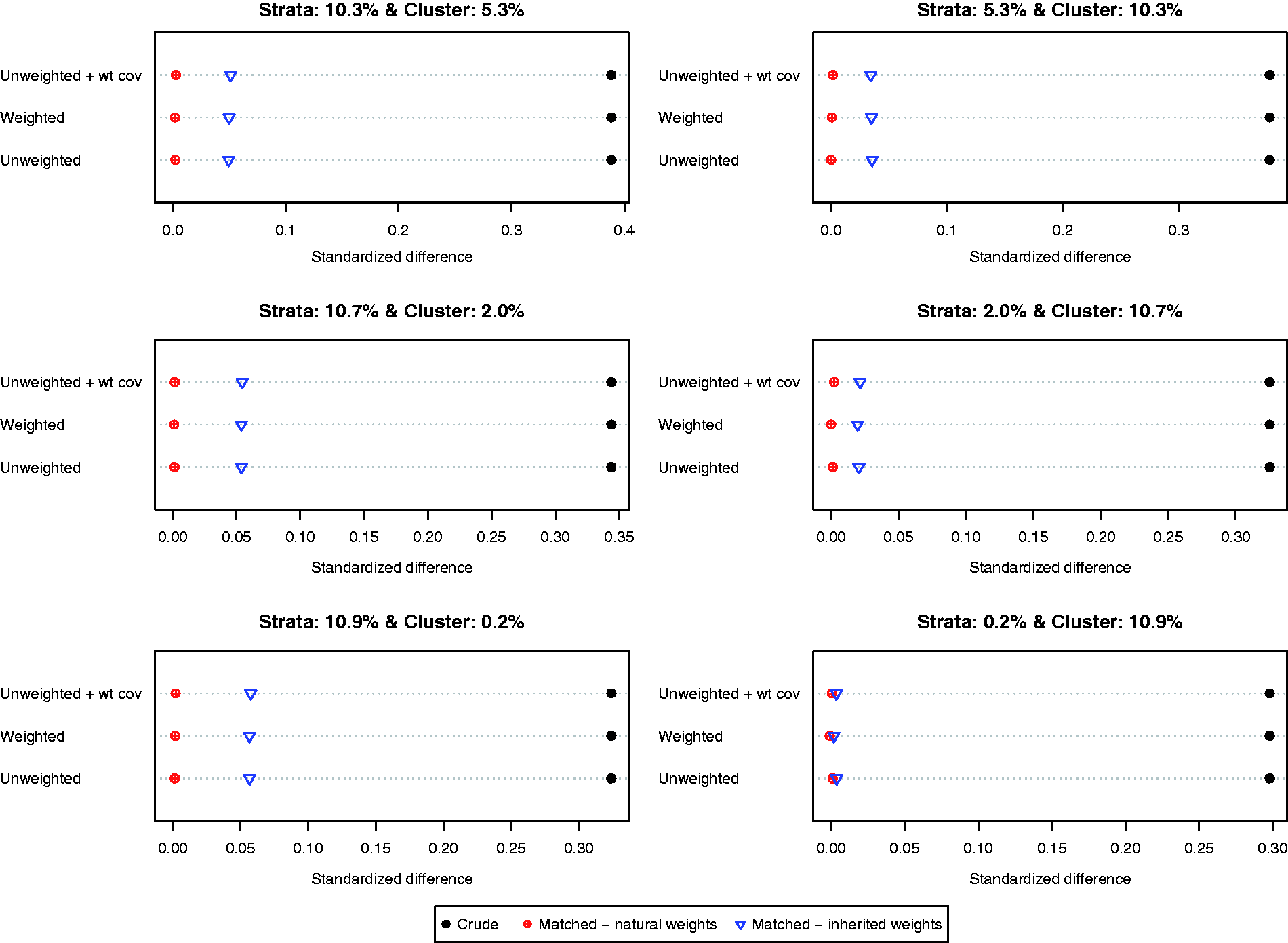

When considering the other five baseline covariates, the difference between the balance induced by the natural weights and that induced by the inherited weights decreased as the original imbalance of the covariate increased. For the last three covariates (X₄, X₅, and X₆), the differences in balance induced by the two different sets of weights were negligible.

4.2 Relative bias in estimated treatment effects

The relative bias of the estimated difference in means for the different methods of implementing propensity score matching is reported in Figure 2 (we report relative bias since the true effect of treatment varied across the six different scenarios due to the heterogeneous effect of treatment). On each of the six dot charts, we have superimposed a vertical line denoting a relative bias of zero. When more variation was due to between-stratum variation compared to between-cluster variation, less bias was observed when using each control subject’s natural weight compared to using each controls subject’s inherited weight, regardless of which of the three specifications of the propensity score model was used. When more variation was due to between-cluster variation compared to between-stratum variation, the results were inconsistent as to which choice of weights resulted in estimates with less bias. However, it must be noted that in these three settings, the relative bias was negligible, regardless of which weights were used. Furthermore, the results were inconsistent as to which specification of the propensity score model resulted in estimates with the lowest relative bias.

Figure 2.

Relative bias in estimated difference in means.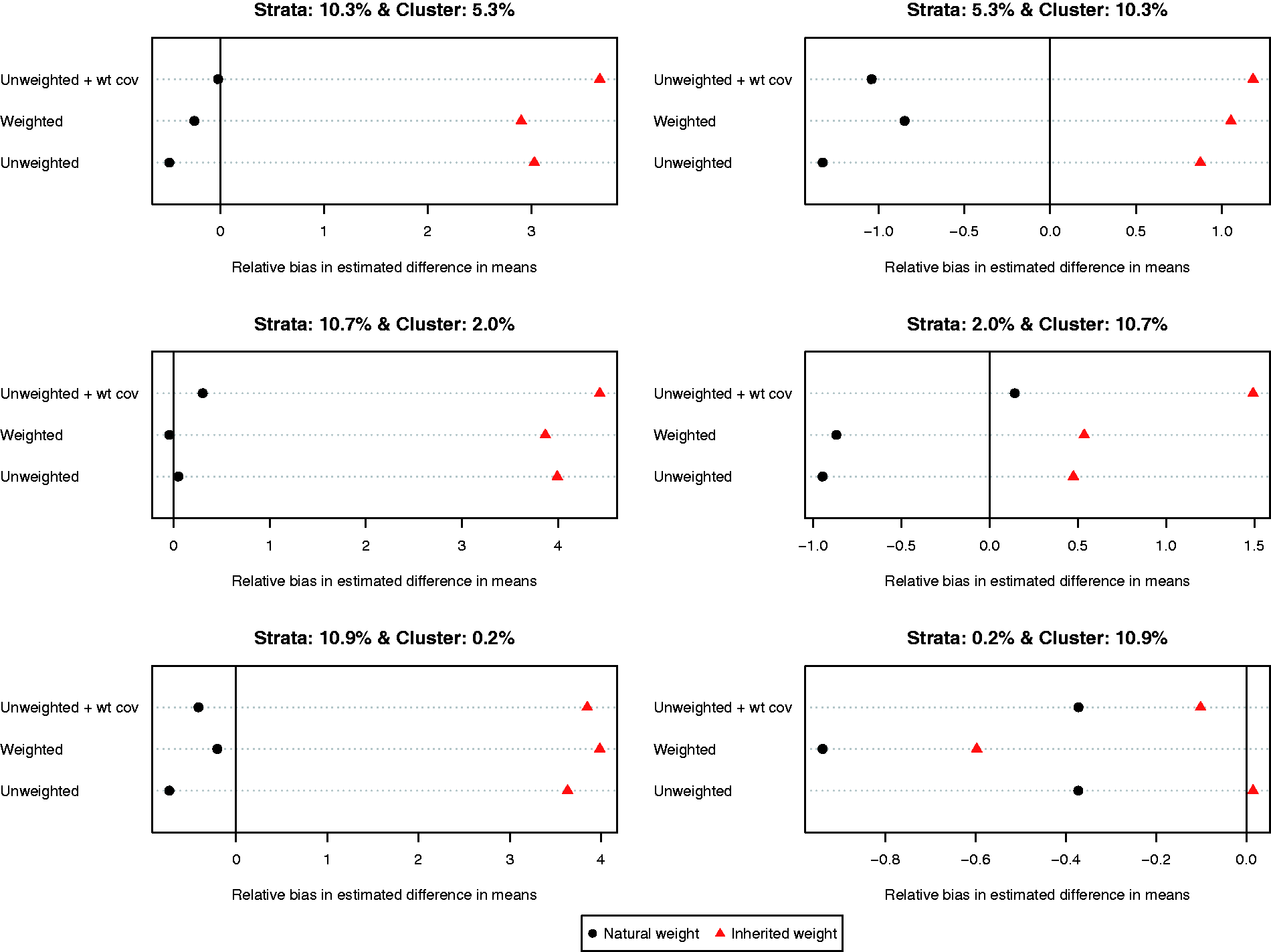

The relative bias of the estimated risk difference for the different methods of implementing propensity score matching is reported in Figure 3. Using each subject’s natural weight tended to result in estimates with less bias compared to using inherited weights. As above, the results were inconsistent as to the preferred specification of the propensity score model.

Figure 3.

Relative bias in estimated risk differences.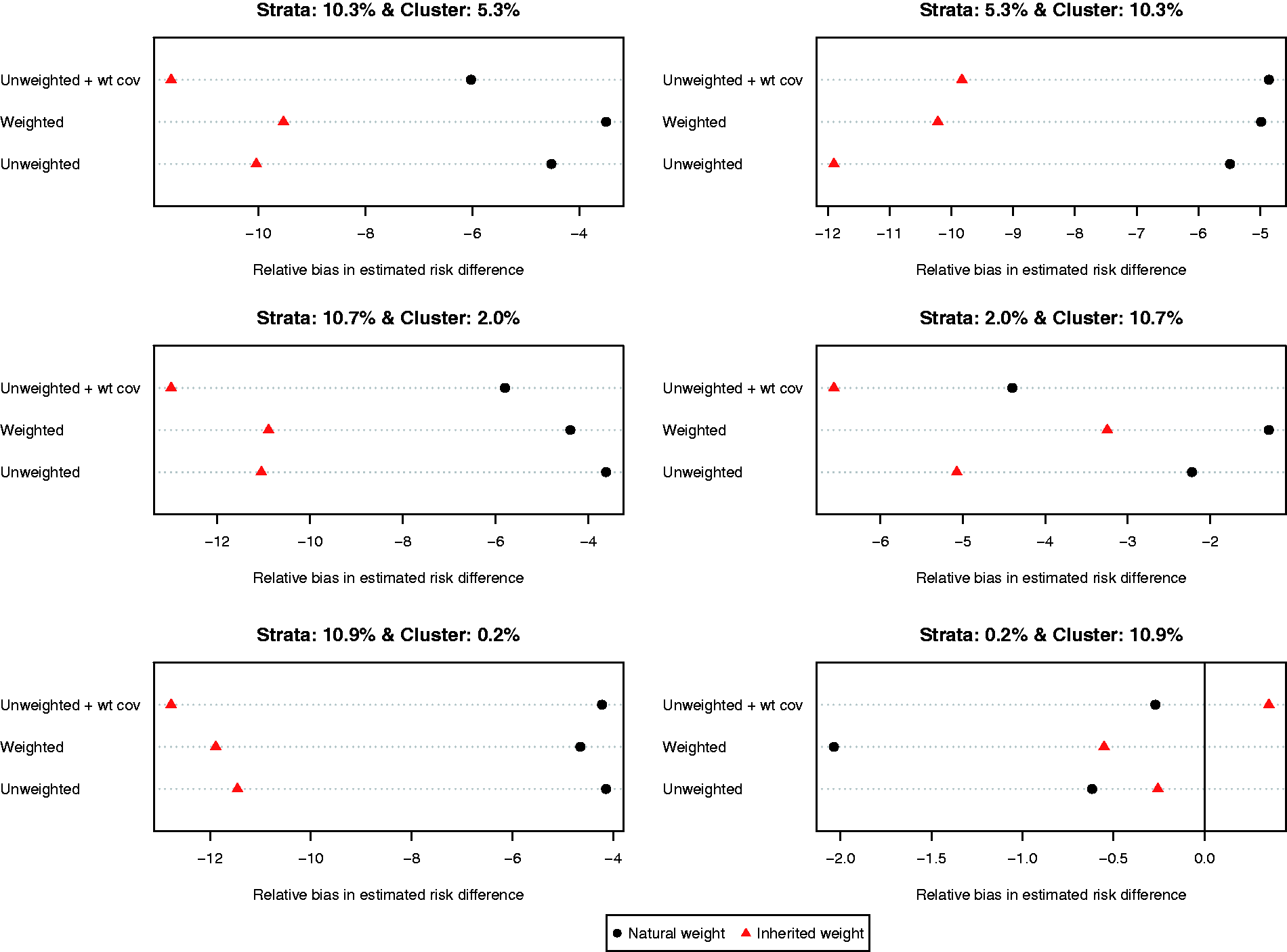

4.3 MSE of estimated treatment effect

The MSEs of the different estimates of the difference in means are reported in Figure 4. MSE tended to be lower when each control subject’s natural weight was used compared to when each control subject’s inherited weight was used. In all six scenarios, the use of a weighted logistic regression model to estimate the propensity score model combined with the use of natural weights resulted in estimates with the lowest MSE.

Figure 4.

MSE of estimated difference in means.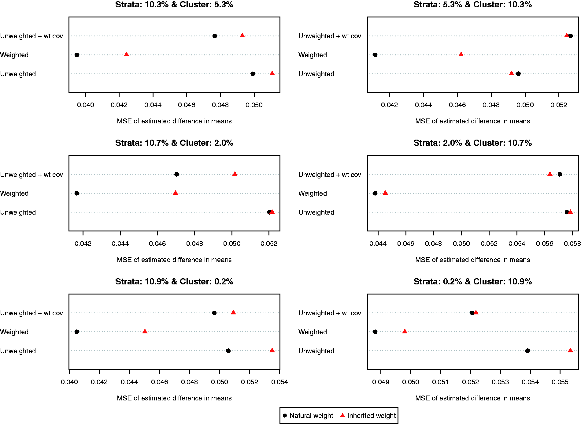

The MSEs of the different estimates of the difference in proportions are reported in Figure 5. Results for the risk difference were less consistent than for the difference in means. In general, the use of natural weights was superior to the use of inherited weights. In general, using a weighted logistic regression to estimate the propensity score combined with the use of natural weights tended to result in estimates with lower MSE compared to other combinations of methods.

Figure 5.

MSE of estimated risk difference.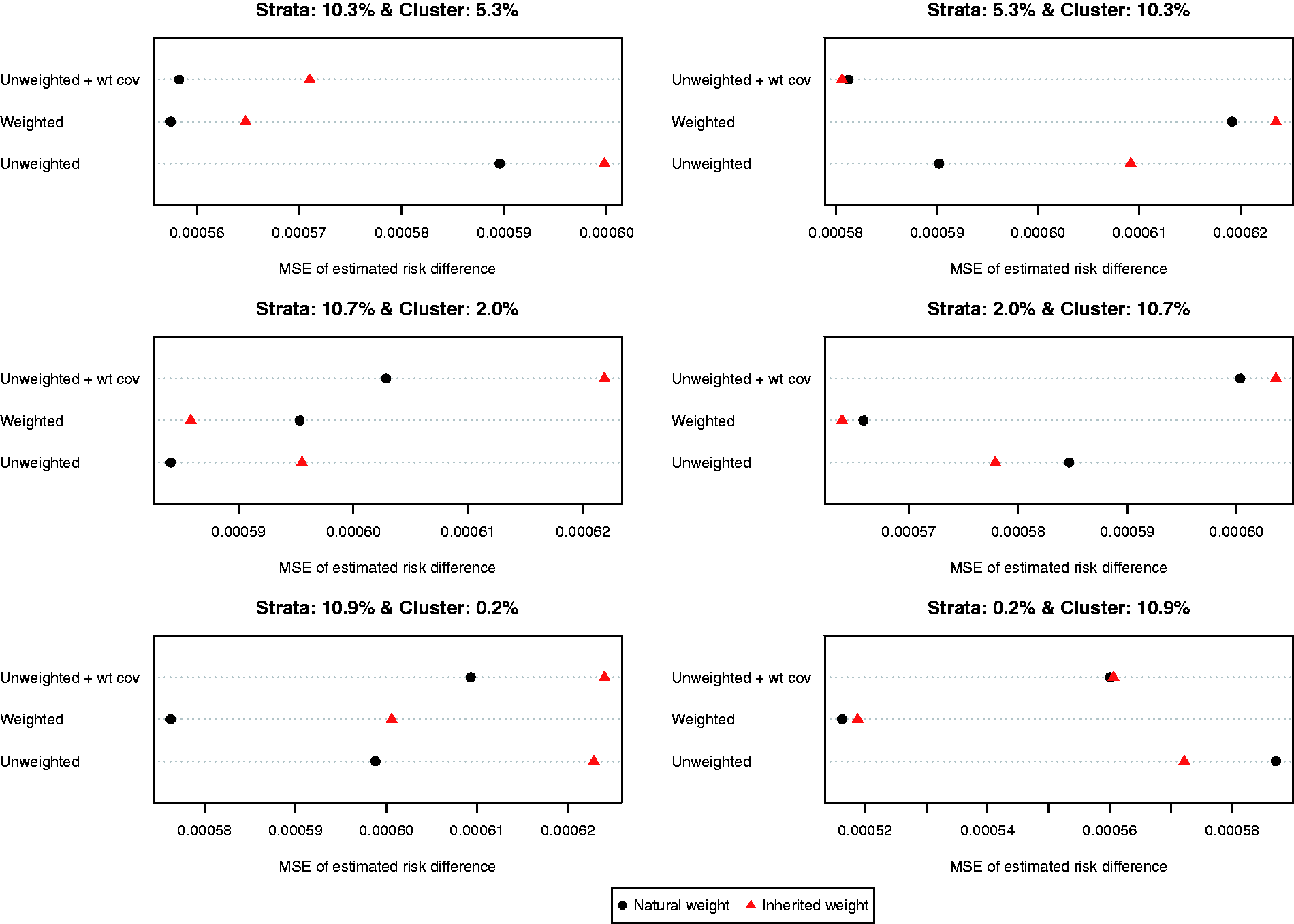

4.4 Variance estimation and 95% confidence intervals

The ratio of the mean estimated standard error to the standard deviation of the estimated difference in means (continuous outcome) across the 1000 simulated datasets is reported in Figure 6. Both choices of weights (natural vs. inherited) and all three propensity score models resulted in estimates of standard error that substantially over-estimated the sampling variability of the estimated treatment effects. This tended to result in estimated 95% confidence intervals that had empirical coverage rates that were higher than the advertised rates (Figure 7). Note that because of our use of 1000 simulated datasets, empirical coverage rates that were lower than 0.9365 or higher than 0.9635 would be statistically significantly different from 0.95 based on a standard normal-theory test.

Figure 6.

Ratio of estimated to empirical standard error (difference in means).

Figure 7.

Empirical coverage rates of 95% CIs (difference in means).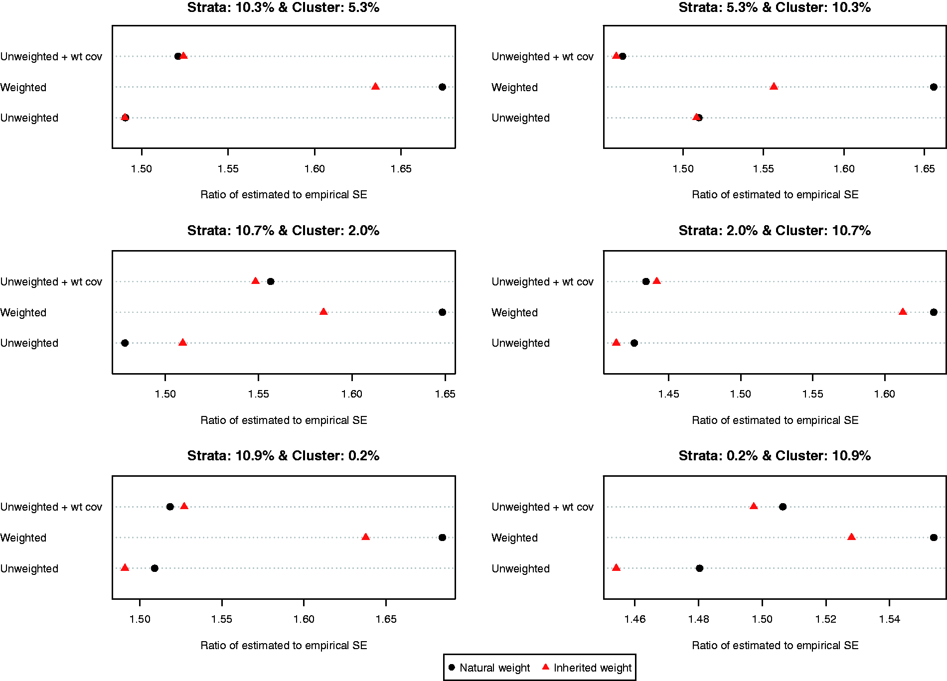

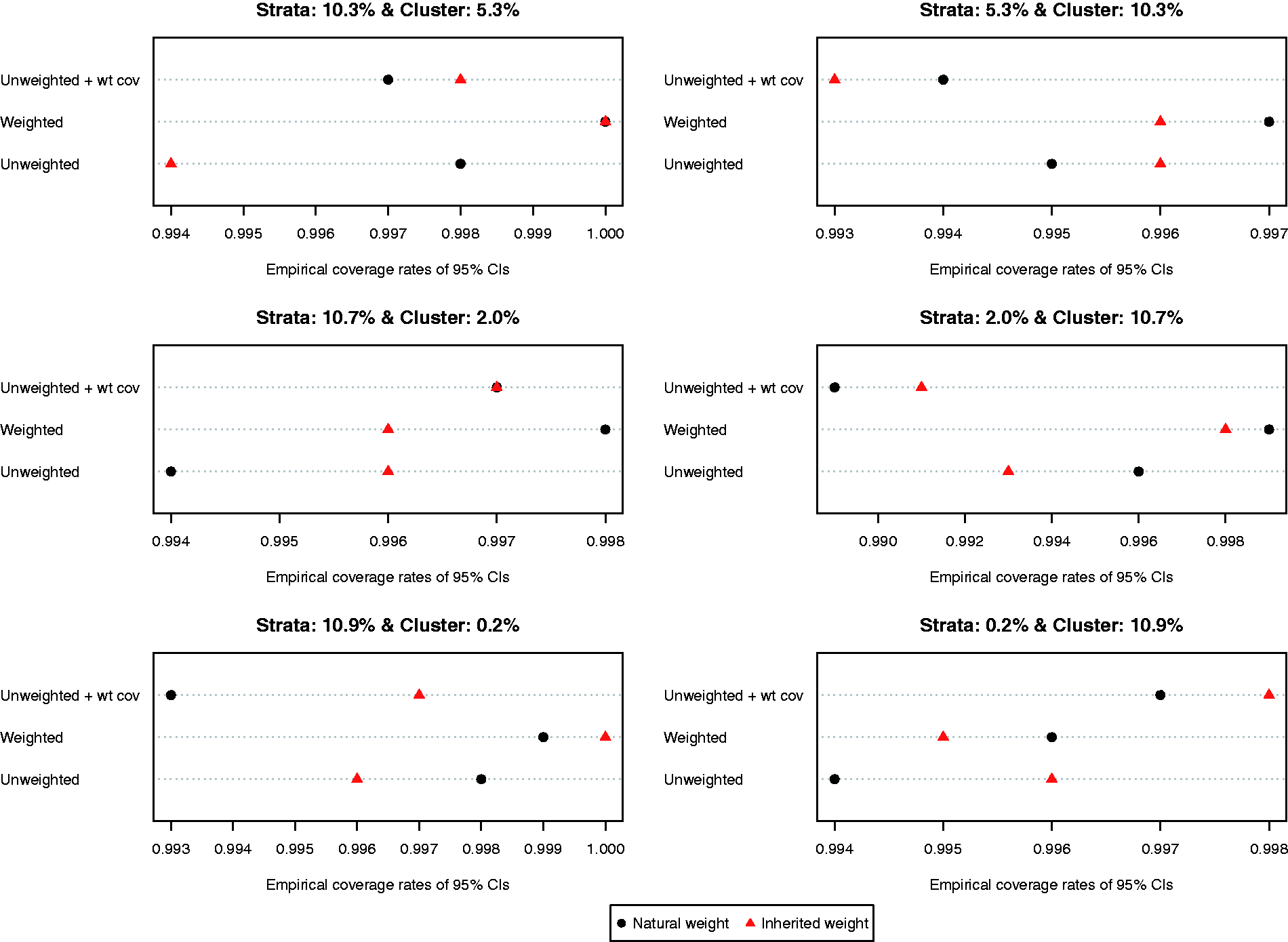
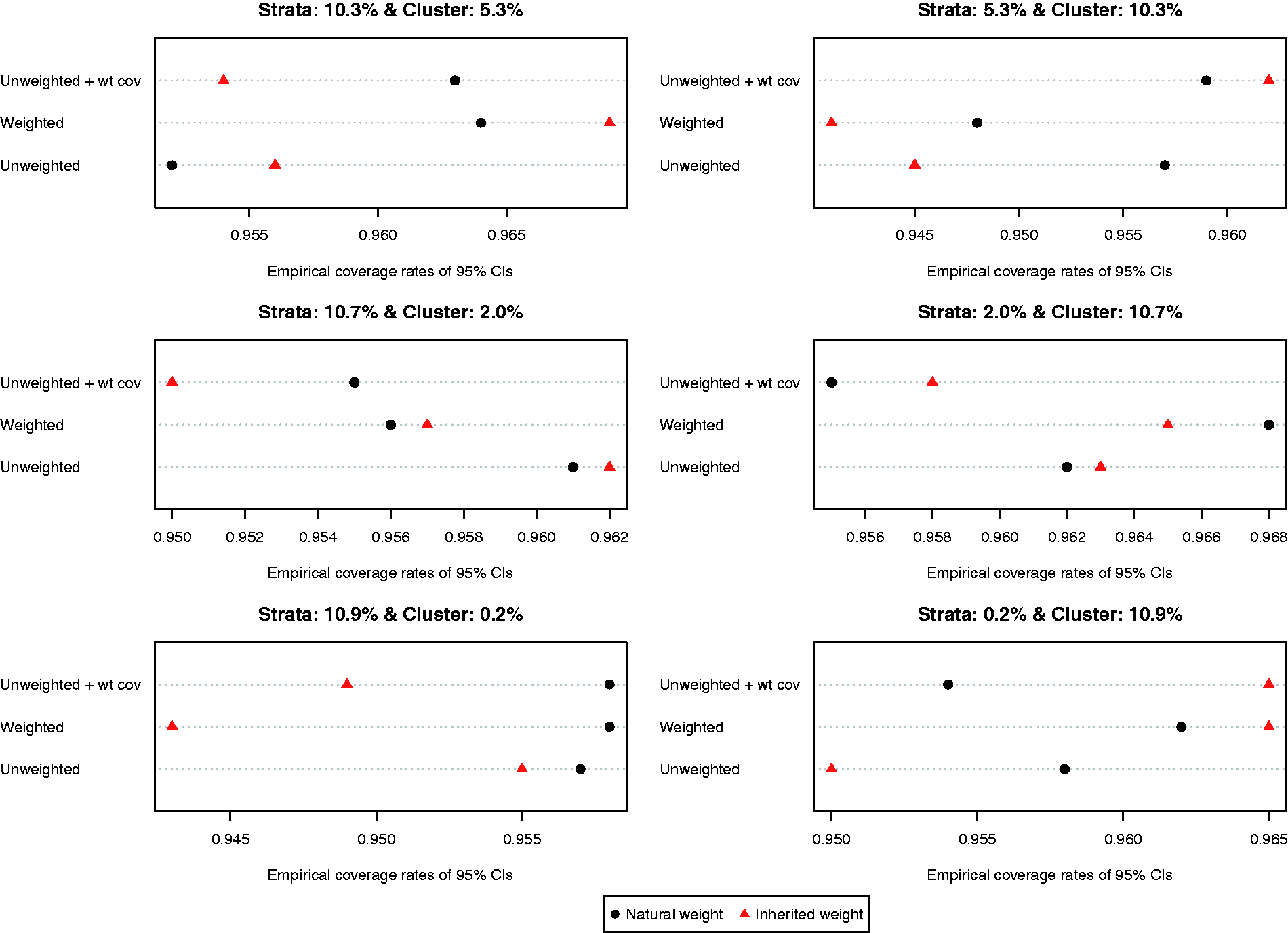
The ratio of the mean estimated standard error to the standard deviation of the estimated difference in proportions (binary outcome) across the 1000 simulated datasets is reported in Figure 8. Compared to the setting with continuous outcomes, the ratios were substantially closer to one, indicating that the bootstrap estimate of variance performed well in the setting with binary outcomes. The results were inconclusive as to which of the six approaches resulted in the most accurate estimates of variance. However, in most of the six scenarios, the differences between the different approaches tended to be modest to minimal. Empirical coverage rates of estimated 95% confidence intervals are reported in Figure 9. In all six scenarios, the majority of methods resulted in confidence intervals whose empirical coverage rates were not statistically significantly different from the advertised rate of 0.95.

Figure 8.

Ratio of estimated to empirical standard error (risk difference).

Figure 9.

Empirical coverage rates of 95% CIs (risk difference).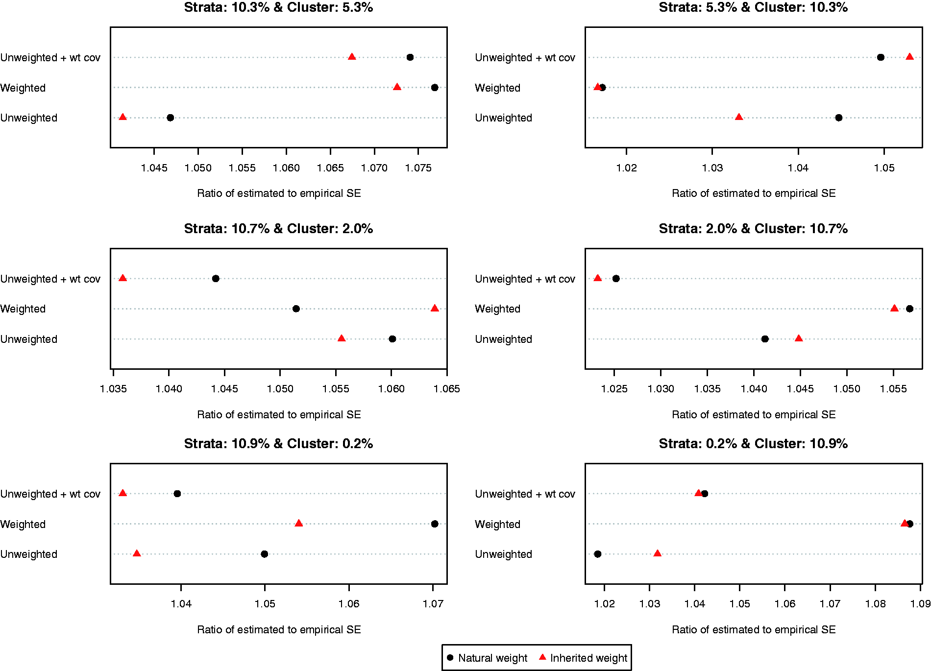

4.5 Sensitivity analysis – DuGoff and Ridgeway scenario

The results of the simulations when using the simulation design described by DuGoff et al. and Ridgeway et al. are reported in Figure 10. Regardless of the method used to estimate the propensity score, lower bias was observed when natural weights were used compared to when inherited weights were used for the matched controls. The difference in bias between using a weighted vs. an unweighted logistic regression model to estimate the propensity score was negligible when natural weights were used. Similarly, the use of natural weights with either a weighted or unweighted logistic regression model to estimate the propensity score resulted in estimates with the lowest MSE. However, the use of inherited weights resulted in more accurate estimates of the standard error of the treatment effect, although the differences were minimal as long as the survey weight was excluded as a covariate from the propensity score model. Finally, the use of natural weights resulted in estimated confidence intervals whose empirical coverage rates were closer to the advertised rate.

Figure 10.

Results for the DuGoff/Ridgeway scenario.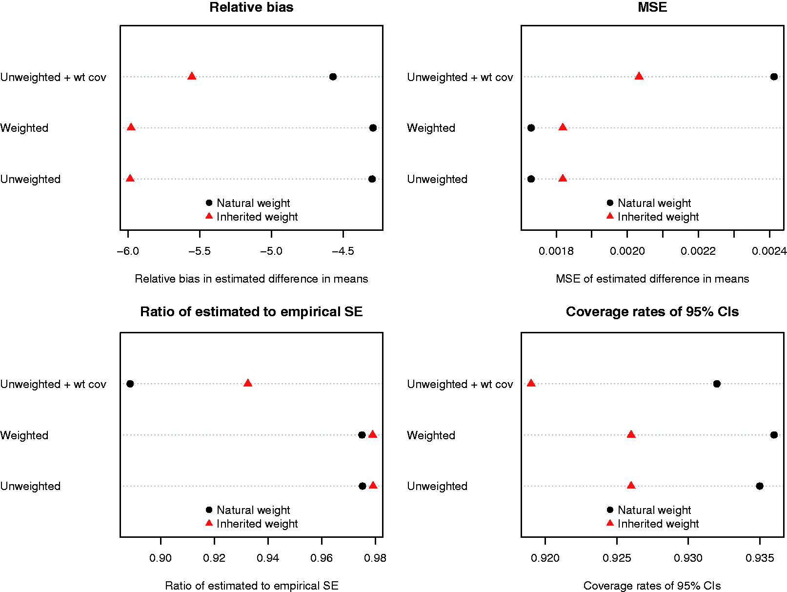

The above findings were similar to those in the primary set of simulations in which lower relative bias and lower MSE tended to be observed when natural weights were used compared to when inherited weights were used for the controls. However, in the sensitivity analyses, we observed that variance estimation using bootstrap-based methods was substantially more accurate than in the primary set of simulations.

5 Case study

We provide a brief empirical example to illustrate the application of the different methods for using propensity score matching with complex survey data.

5.1 Data sources

The CCHS is a cross-sectional survey used to collect information on health status and determinants of health of the Canadian population. It includes individuals aged 12 years or over living in private dwellings. The surveys excluded institutionalized persons, as well as those living on native reservations and full-time members of the Canadian Forces. Our study sample included 161,844 adults aged 20 years or older who participated in the Ontario components of the CCHS between 2001 and 2013.

The exposed group was defined as those who self-reported less than high school education and the control group was defined as those who self-reported at least the completion of high school. In our study sample, 22,487 were exposed, with the remaining 139,357 subjects serving as controls. The outcome was self-reported mood (e.g. depression, bipolar disorder, mania or dysthymia) or anxiety (e.g. a phobia, obsessive compulsive disorder or a panic disorder) disorders diagnosed by a health professional prior to the interview date. The covariates included age group (20–29 years, 30–39 years, 40–49 years, ≥50 years); sex; household income (<$30,000, $30,000 to <$60,000, $60,000 to <$80,000, ≥$80,000); urban/rural dwelling; work status (employed vs. unemployed in the past year); current smoking; alcohol consumption (non-drinker vs. moderate drinker vs. heavy drinker); inadequate fruit and vegetable consumption (fewer than three times per day); physical inactivity (energy expenditure <1.5 kcal per kg weight per day); sense of belonging to the local community (somewhat weak or very weak vs. very strong or somewhat strong); and the presence of two or more physician-diagnosed chronic conditions.

5.2 Statistical analyses

We used the three different methods to estimate the propensity score that were considered in the simulations. Using each of the three propensity score models, a matched sample was constructed using nearest neighbor caliper matching on the logit of the propensity score using calipers of width equal to 0.2 of the standard deviation of the logit of the propensity score.^14,15,20 Subjects were matched only on the propensity score and not on stratum or cluster, as these identifiers were not available.

In each of the six matched samples, balance in the measured baseline covariates was assessed using standardized differences estimated in the weighted sample. ²³ The effect of exposure on the outcome was determined by estimating the prevalence of the outcome in exposed and control subjects separately in the matched sample. Estimation of prevalence incorporated the sampling weights. We estimated the effect of treatment using both natural weights and inherited weights for the matched control subjects. The effect of exposure was quantified as the difference in the proportion of exposed subjects who experienced the outcome and the proportion of control subjects who experienced the outcome. Bootstrap methods were used to construct 95% confidence intervals for the estimated effect estimates.

5.3 Results

When the propensity score model was estimated using an unweighted logistic regression model, 22,466 exposed subjects were matched to a control subject (99.91% of the exposed subjects were successfully matched). When the propensity score was estimated using a weighted logistic regression model, 22,485 (99.99%) exposed subjects were matched to a control subject. When the propensity score model was estimated using an unweighted logistic regression model that included the survey weight as an additional covariate, 22,470 (99.92%) exposed subjects were matched to a control subject.

The results of the empirical analyses are reported in Table 1. In general, all six matching methods resulted in good balance on the measured baseline covariates. However, one method resulted in noticeably worse balance that the other five methods. When the sampling weight was included as an additional covariate in the propensity score model and the matched control subject inherited the sampling weight of the control to whom they were matched, then some residual imbalance was observed for a few covariates. When using this approach, the standardized differences for the covariate denoting physical inactivity and rural residence took on the following values 0.100 and −0.125. Apart from these two values, all 112 other standardized differences ranged from −0.057 to 0.072. These results reflect our findings from the Monte Carlo simulations in which we observed that worse balance was induced by using the inherited weights than was induced by allowing each matched control subject to retain their natural sampling weight. Furthermore, our empirical results reflect the findings of the simulations, in which we observed that the formulation of the propensity score model had negligible impact on baseline balance.

Table 1.

Balance in baseline covariates and estimated risk differences for the six different approaches to propensity score matching in the CCHS sample.

Variable	Specification of propensity score model
	Unweighted logistic regression model		Weighted logistic regression model		Unweighted logistic regression model + survey weight as an additional covariate
	Retained weights	Inherited weights	Retained weights	Inherited weights	Retained weights	Inherited weights
Standardized differences
Age 20–29 years	−0.010	0.007	−0.018	0.013	−0.017	0.007
Age 30–39 years	0.026	0.001	0.020	0.001	0.015	0.009
Age 40–49 years	−0.008	−0.002	−0.008	0.001	−0.007	0.011
Age ≥50 years	−0.011	−0.008	0.007	−0.020	0.011	−0.034
Two or more chronic conditions	0.006	−0.004	0.008	0.003	0.022	0.016
Ate fruits and vegetables  <3 times per day	0.002	0.002	0.001	0.008	−0.008	−0.010
Income less than $30,000	−0.018	0.001	−0.017	0.006	−0.033	−0.001
Income between $30,000 and $60,000	−0.002	−0.005	−0.009	−0.008	−0.009	−0.015
Income between $60,000 and $80,000	0.019	0.000	0.009	−0.002	0.012	−0.011
Income greater than $80,000	−0.001	0.004	0.016	0.004	0.027	0.026
Male	−0.045	−0.003	−0.030	−0.003	−0.028	0.021
Physically inactive	−0.001	0.002	0.008	0.004	0.012	0.100
Rural dwelling	0.001	0.000	0.003	−0.007	0.012	−0.125
Poor sense of belonging	−0.010	0.003	−0.011	0.011	−0.007	0.001
Current smoking	−0.013	0.000	−0.026	0.001	0.015	0.008
Non-drinker	0.006	0.005	0.023	0.011	0.011	0.072
Moderate drinker	−0.023	−0.004	−0.042	−0.009	−0.036	−0.057
Heavy drinker	0.013	−0.002	0.013	−0.003	0.019	−0.024
Work status (unemployed in past year)	−0.008	−0.010	−0.020	−0.011	−0.005	−0.031
Effect of low education on the probability of a prevalent mood or anxiety disorder
Difference in probability of prevalent  mood or anxiety disorder (95% CI)	−0.005 (−0.017, 0.006)	−0.013 (−0.025, −0.001)	−0.013 (−0.025, 0)	−0.02 (−0.031, −0.008)	−0.012 (−0.026, 0.002)	−0.018 (−0.033, −0.003)

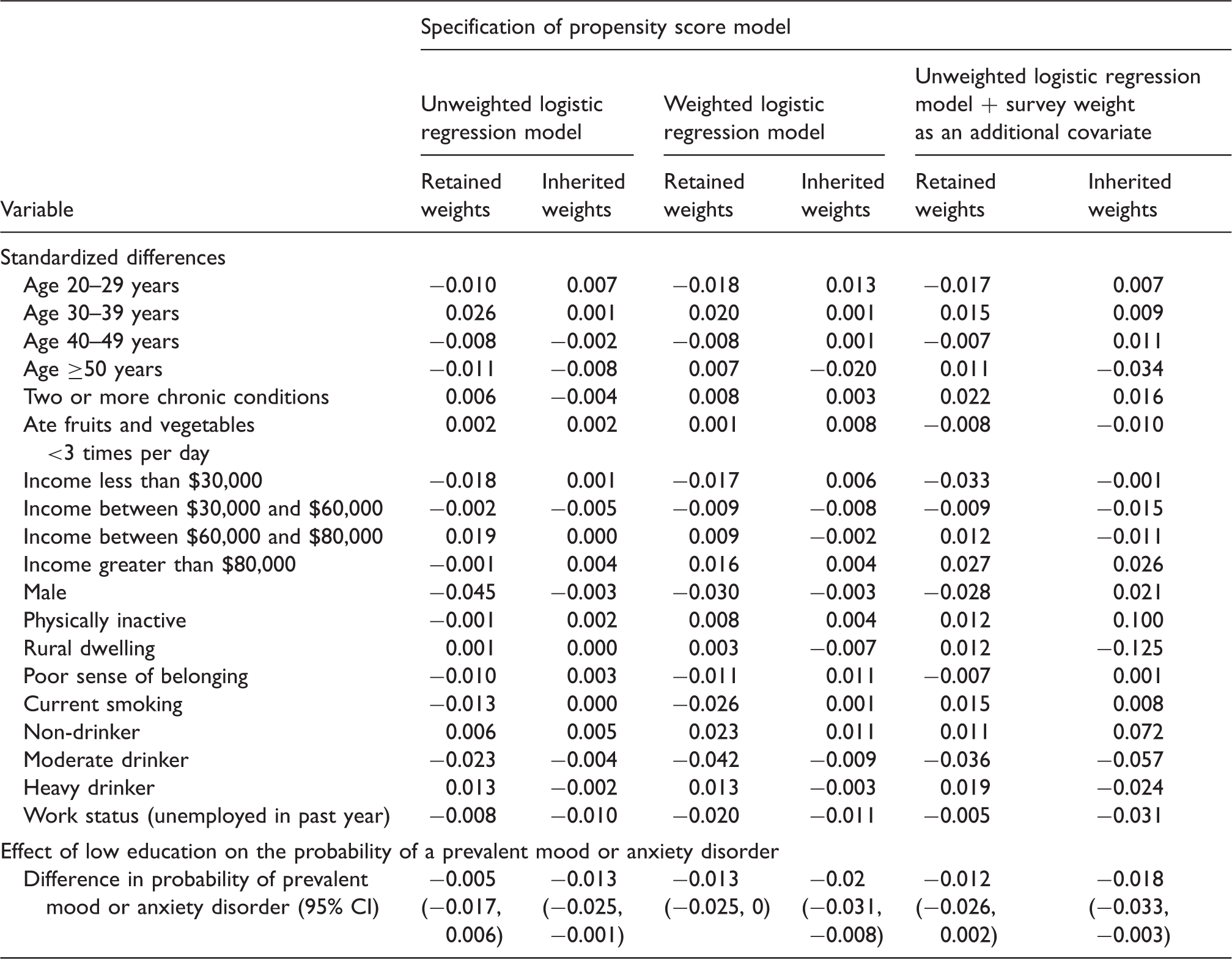
The estimated risk differences ranged from −0.02 to −0.005. The point estimates are negative, indicating that subjects with less than high school education have a decreased probability of having a self-reported physician-diagnosed mood or anxiety disorder. For each method of estimating the propensity score, the use of inherited weights resulted in an effect estimate of greater magnitude than did the use of the natural weights. In the Monte Carlo simulations, we observed that less bias tended to be observed when using each control subject’s natural weight compared to using each controls subject’s inherited weight, regardless of which of the three specifications of the propensity score model was used. This suggests that, in our empirical analyses, the estimates of smaller magnitude (i.e. those obtained using the natural weights) are likely closer to the truth than are the larger estimates (i.e. those obtained using inherited weights).

6 Discussion

We conducted an extensive series of Monte Carlo simulations to examine two issues that must be addressed when using propensity score matching with complex survey data to estimate population treatment effects. The first issue that we considered was the formulation of the propensity score model. We considered three different methods of estimating the propensity score, depending on whether or not a weighted regression model was fit and whether or not the survey weights were incorporated as an additional covariate in the propensity score model. None of the three different propensity score models resulted in appreciably better balance of baseline covariates than other specifications of the propensity score model. Our results were inconsistent as to which specification of the propensity score model resulted in estimates with the lowest bias or MSE. The second issue that we considered was whether matched control subjects should inherit the sampling weight of the treated subject to whom they were matched, or whether they should retain their natural sampling weight. Better balance on measured baseline covariates was induced by using each control subject’s natural weight than was induced by allowing each matched control subject to inherit the sampling weight of the treated subject to whom they were matched. Similarly, we found that the use of natural weights tended to result in estimates with lower bias and lower MSE compared to the use of inherited weights. When outcomes were continuous, the use of a weighted logistic regression model to estimate the propensity score combined with the use of natural weights resulted in estimates with the lowest MSE.

As described in Section 2.1, both DuGoff et al. ⁶ and Ridgeway et al. ⁷ used Monte Carlo simulations to examine estimation of treatment effects using propensity score methods with sample surveys. The simulation designs of these two earlier papers were similar to one another: the population was comprised three strata, and there was a single measured baseline covariate. The simulation design in the current study was substantially more complex, with the population being divided into ten strata, each of which was comprised of 20 clusters. Thus, the current design reflects the stratified cluster sample which is more frequently employed for large nationally representative health surveys. Furthermore, rather than a single confounding variable, we considered the setting with six confounding variables, such that the distribution of these variables varied across strata and clusters. As a sensitivity analysis, we repeated our simulations using a data-generating process described in these two previous studies.

As noted in Section 2, DuGoff et al. suggested that estimation of the propensity score model does not incorporate the sampling weights, while Ridgeway et al. disagreed with this assertion. Our findings on this issue were inconsistent, with no method of estimation being clearly preferable to the others.

In the current study, we evaluated the performance of different methods of using propensity scores with sample surveys by assessing covariate balance on baseline covariates, bias in the estimated treatment effect, variance estimation, and the MSE of the estimated treatment effect. We examined the use of bootstrap-based methods for estimating variance. Variance estimation when using propensity score matching with a sample survey is complex for two intersecting reasons. First, variance estimation when using a sample survey needs to account for the design of the survey. ⁴ Thus, information about membership of subjects in strata and clusters needs to be accounted for when estimating the variance of estimated statistics. Second, variance estimation when using conventional propensity score matching with simple random samples needs to account for the matched nature of the sample.^26–29 Methods for variance estimation in a propensity score matched sample constructed from a stratified cluster sample have not been described and further research is required in this area. Variance estimation would need to account for both the within-matched sets correlation in outcomes as well as the design of the sample survey. In our Monte Carlo simulations, we examined the performance of a bootstrap-based approach for estimating the standard error of estimated treatment effect. This approach performed well when the outcome was binary, and the risk difference was used as the measure of treatment effect. However, this approach resulted in inflated estimates of standard error when the outcome was continuous. Further research is necessary to determine methods to improve variance estimation in settings with continuous outcomes.

One of the results of the current study that may be surprising to some readers was that the use of natural weights for matched control subjects tended to result in superior performance compared to the use of inherited weights for these matched control subjects. When the treated subjects in the matched sample are weighted using their natural weights, then the target population is the population of treated subjects. The use of the treated subjects’ weights with the matched treated subjects results in the standardization of the matched treated subjects to the population of treated subjects. The sample of matched control subjects resembles the sample of matched treated subjects. The use of natural weights with the matched control subjects results in the sample of matched control subjects being standardized to the population of control subjects who resemble the population of treated subjects. Thus, the use of natural weights permits the comparison of outcomes in the population of treated subjects with the population of control subjects who resemble the treated subjects. This analytic choice was implicitly made in the only previous study to examine the use of propensity score matching with complex surveys. In that study, DuGoff et al. ⁶ used a weighted regression model to regress the outcome on an indicator variable denoting treatment status and the single baseline covariate. In doing so, they were implicitly using natural weights, as the weights for the matched control subjects were not replaced by the inherited weights.

In summary, we recommend that when using propensity score matching with complex surveys, that the matched control subjects retain their natural weight, rather than inheriting the survey weight of the treated subject to whom they were matched.