Sage Journals: Discover world-class research

Abstract

Propensity score methods are frequently used to estimate the effects of interventions using observational data. The propensity score was originally developed for use with binary exposures. The generalized propensity score (GPS) is an extension of the propensity score for use with quantitative or continuous exposures (e.g. pack-years of cigarettes smoked, dose of medication, or years of education). We describe how the GPS can be used to estimate the effect of continuous exposures on survival or time-to-event outcomes. To do so we modified the concept of the dose–response function for use with time-to-event outcomes. We used Monte Carlo simulations to examine the performance of different methods of using the GPS to estimate the effect of quantitative exposures on survival or time-to-event outcomes. We examined covariate adjustment using the GPS and weighting using weights based on the inverse of the GPS. The use of methods based on the GPS was compared with the use of conventional G-computation and weighted G-computation. Conventional G-computation resulted in estimates of the dose–response function that displayed the lowest bias and the lowest variability. Amongst the two GPS-based methods, covariate adjustment using the GPS tended to have the better performance. We illustrate the application of these methods by estimating the effect of average neighbourhood income on the probability of survival following hospitalization for an acute myocardial infarction.

Keywords

Propensity score generalized propensity score quantitative exposure observational study survival analysis

1 Introduction

Observational data are increasingly being used to estimate the effects of treatments, interventions, and exposures. When conducting observational studies, analysts must account for the confounding that occurs when the distribution of baseline covariates differs between exposed and control subjects. Appropriate statistical methods must be used to account for this confounding so that valid conclusions about the effects of exposures can be drawn. Analysts frequently use methods based on the propensity score to account for the confounding that occurs in observational studies.^1,2

The propensity score was developed initially for use with binary treatments or exposures (e.g. treatment vs. control). However, propensity score methods have subsequently been extended to allow analysts to estimate the effect of continuous or quantitative exposures.^3–5 Examples of quantitative exposures include dose of medication used, pack-years of cigarettes smoked, body mass index (BMI), or duration of job tenure. The extension of propensity score methods to continuous exposures has been referred to as the generalized propensity score (GPS).^5,6

The original methods papers that introduced the GPS considered continuous outcomes such as labor earnings,^5,6 medical expenditures,⁴ and birth weight.⁷ In biomedical research, survival or time-to-event outcomes occur frequently (e.g. time to death or time to incidence of disease).⁸ Despite the frequency of survival outcomes and the increased use of the GPS, there are, to the best of our knowledge, no studies examining the performance of the GPS for estimating the effect of continuous or quantitative exposures on time-to-event outcomes.

The objective of the current study was two-fold. First, to describe different methods for using the GPS to estimate the effect of continuous or quantitative exposures on time-to-event outcomes. Second, to evaluate the relative performance of these different methods. The paper is structured as follows: In Section 2, we provide notation, a brief background on the GPS, and describe methods for using the GPS to estimate the effect of continuous exposures on time-to-event outcomes. In Section 3, we provide a case study to illustrate the application of GPS-based methods to estimate the effect of average neighbourhood income on survival within one year of hospital admission using a sample of patients hospitalized with acute myocardial infarction (AMI). In Section 4, we use Monte Carlo simulations to evaluate the performance of these methods. Finally, in Section 5, we summarize our findings and place them in the context of the existing literature.

2 Using the generalized propensity score with time-to-event outcomes

In this section, we introduce the GPS and describe two ways in which it can be used to estimate the dose–response function for a quantitative exposure and time-to-event outcomes.

2.1 The generalized propensity score

We use the following notation throughout the paper. Let Z denote a quantitative or continuous variable denoting the level of exposure (e.g. income), and let X denote a vector of measured baseline covariates. Using the terminology of Hirano and Imbens, let $r (z, x)$ denote the conditional density of the continuous exposure variable given the measured baseline covariates:

r (z, x) = f_{Z | X} (z | x)

(1)

Then the generalized propensity score is $R = r (Z, X)$ .⁵ Imai and van Dyk refer to the conditional density function f_Z_|X as the propensity function.⁴ The propensity function can be estimated by regressing the quantitative exposure on the set of observed baseline covariates. This is frequently done using ordinary least squares (OLS) regression. When using OLS regression, one can determine the density function of the conditional distribution of the continuous exposure by using the estimated regression coefficients and the estimated residual variance. For a given subject, the subject’s value of the GPS is the density function evaluated at the observed value of that subject’s exposure. If the exposure Z is normally distributed with mean $β^{T} x$ and variance $σ^{2}$ (where β and σ² are estimated using OLS estimation), then $f_{Z | X} (z | x)$ can be estimated by the normal density $\frac{1}{\sqrt{2 π {\hat{σ}}^{2}}} e^{- \frac{(z - {\hat{β}}^{T} x)^{2}}{2 {\hat{σ}}^{2}}}$ where z denotes the observed value of the subject’s exposure.⁹ This is the subject’s value of the GPS. The assumption that the conditional distribution of the exposure is normal is often used as a simplifying assumption or as a reasonable approximation. However, the assumption of normality is not required. As an alternative to OLS regression, one could use a generalized linear model.¹⁰ The important issue is that one model the relationship between the quantitative exposure and be able to parametrically describe the density function of the quantitative exposure conditional on the baseline covariates.

2.2 Estimation of the dose–response function using the generalized propensity score

The GPS assumes the existence of a set of potential outcomes, $Y_{i} (z), for z \in Ψ,$ where $Y_{i} (z)$ denotes the outcome of the ith subject if they received exposure $Z = z$ , while Ψ denotes the set of all possible values of the exposure. In the conventional setting with a dichotomous exposure, $Ψ = {0, 1} .$ The dose–response function is defined as $μ (z) = E [Y_{i} (z)]$ . This dose–response function denotes the average response in the population (or sample) if all subjects were to receive $Z = z$ . By comparing $μ (z_{1})$ with $μ (z_{2})$ , one can estimate the mean change in the outcome if all subjects were exposed to $Z = z_{2}$ instead of $Z = z_{1}$ . A variety of methods have been proposed for using the GPS to estimate the dose–response function.^3,5–7,11

With time-to-event outcomes, we suggest that the concept of the dose–response function requires modification. If one were to use the definition of the dose–response function used for continuous or binary outcomes, then the value of the dose–response function for a given value of exposure would denote the mean or expected survival time under that value of the continuous exposure. There are two limitations to this approach. The first limitation is that, in practice, it can be difficult to estimate mean survival in the presence of a moderate to high degree of censoring. The second limitation is that in many applied areas, differences in survival are often not quantified using differences in mean or expected survival. Instead, differences in survival are often quantified using differences in the survival function or differences in the probability of survival to pre-specified time points. For these two reasons, we propose that the dose–response function be modified so that $μ (z) = S (t | z)$ . Thus, the dose–response function for a given value of the continuous exposure denotes the survival function if all subjects in the sample or population were to receive the given value of the exposure. Formally, one could speak of a dose–response surface: $μ (z, t) = S (t | z)$ . However, we retain the term ‘dose–response function’ for consistency with other types of outcomes. One must bear in mind that the value of the dose–response function is the survival function associated with the given value of the continuous exposure variable.

We will focus on two approaches to estimate the dose–response function with time-to-event outcomes: covariate adjustment using the GPS and weighting using the inverse of the GPS. With survival outcomes, the dose–response function relates the value of the continuous or quantitative exposure to the survival function, which denotes the probability of the occurrence of the event prior over time.

When using covariate adjustment using the GPS, one regresses the hazard of the occurrence of the event on the quantitative exposure variable and the estimated GPS (estimated at the observed value of the quantitative exposure variable) using a Cox proportional hazards regression model.^5,6 Let $log (h (t)) = h_{0} (t) + β_{1} Z + β_{2} GPS$ denote the Cox proportional hazards model where $h (t)$ denotes the hazard function, $h_{0} (t)$ denotes the baseline hazard function (the hazard function for a subject for whom both Z and GPS are equal to zero), Z denotes the observed quantitative exposure variable, and GPS denotes the generalized propensity score (evaluated at the subject’s observed value of the quantitative exposure variable). Based on the fitted regression model, one can then estimate the expected survival function for a given subject if their exposure was set equal to $Z = z$ . Let $S_{0} (t)$ denote the Breslow estimate of the baseline survival function.¹² Then we have that $S (t | z) = S_{0} (t)^{e^{β_{1} z + β_{2} {GPS}_{z}}}$ (we use the term ${GPS}_{z}$ to denote the value of the GPS for a given subject at the exposure value Z = z, and not at the subject’s observed exposure level). By taking the mean of this estimated survival function over the study sample, one can estimate the dose–response function: $μ (z, t) = S (t | z)$ .

Both Imbens and Robins et al. suggested that weights could be derived from the GPS. These weights can then be used to estimate the dose–response function.^3,7 Weights can be defined as $\frac{W (Z_{i})}{r (Z_{i} | X_{i})}$ , where the numerator is a function that is included to stabilize the weights. It has been suggested that a reasonable choice for W is an estimate of the marginal density function of Z.⁷ The marginal density function can be determined by calculating the mean and the variance of the quantitative exposure variable in the overall sample ( $μ_{sample}$ and $σ_{sample}^{2}$ , respectively). Then $W (Z_{i}) = \frac{1}{\sqrt{2 π σ_{sample}^{2}}} e^{- \frac{(Z_{i} - μ_{sample})^{2}}{2 σ_{sample}^{2}}}$ .⁹ Once the GPS-based weights have been estimated, a univariate Cox proportional hazards regression model can be fit in which the hazard of the occurrence of the outcome is regressed on the continuous exposure using a weighted regression model that incorporates the GPS-based weights. From the fitted outcomes model, the dose–response function can be estimated by calculating the expected survival function across all levels of exposure.

3 Case study

We conducted an analysis of data to estimate the effect of average neighbourhood income on survival within one year of hospitalization for an AMI. This analysis was conducted for two reasons. First, to illustrate the application of the methods described above to estimate the dose–response function for survival outcomes. Second, the results of the data analysis informed the design of the Monte Carlo simulations used in the following section to assess the performance of the proposed methods.

3.1 Data and analyses

We used data consisting of 10,007 patients hospitalized with an AMI in Ontario, Canada between April 1999 and March 2001. These data were collected as part of the Enhanced Feedback for Effective Cardiac Treatment Study.¹³ These data were linked to census data from Statistics Canada to determine the average neighbourhood income for each subject and to the Registered Persons Database to determine the date of death of each subject who died subsequent to hospitalization for AMI. Average neighbourhood income was used as the continuous exposure variable in this case study. The nine deciles of average neighbourhood income were $24,860, $26,144, $26,914, $28,068, $28,985, $32,237, $32,364, $34,723, and $38,891. The standard deviation of the average neighbourhood income was $8,133. For the purposes of regression modeling, average neighbourhood income was standardized to have mean zero and unit variance. For the current case study, we considered a time-to-event outcome defined as the time from hospital admission to date of death. Subjects were followed for up to one year, and were censored after 365 days if they were still alive.

The propensity function was estimated by regressing standardized average neighbourhood income on a set of 34 baseline covariates using a linear regression model estimated using OLS. The 34 baseline covariates included demographic characteristics (age and sex), vital signs on admission (systolic and diastolic blood pressure, respiratory rate, and heart rate), initial laboratory values (white blood count, hemoglobin, sodium, glucose, potassium, and creatinine), signs and symptoms on presentation (acute congestive heart failure and cardiogenic shock), classic cardiac risk factors (family history of heart disease, current smoker, history of hyperlipidemia, and hypertension), and comorbid conditions (chronic congestive heart failure, diabetes, stroke or transient ischemic attack, angina, cancer, dementia, previous AMI, asthma, depression, hyperthyroidism, peptic ulcer disease, peripheral vascular disease, previous coronary revascularization, history of bleeding, renal disease, and aortic stenosis). Each of the 11 continuous baseline covariates was standardized to have mean zero and unit variance.

We computed the nine deciles of the continuous exposure (standardized average neighbourhood income). We then used the methods described in Section 2 to estimate the dose–response function at these nine deciles of standardized average neighborhood income. When using covariate adjustment using the GPS, the hazard of death was regressed on the GPS and standardized average neighbourhood income and the interaction between these two terms.

For comparative purposes, we examined two alternative methods of estimating the dose–response function. The first alternative method was based on G-computation.¹⁴ When using this approach, a Cox proportional hazards regression model was used to regress the hazard of death on standardized average neighbourhood income and the 34 baseline covariates. We then created nine synthetic datasets, each of which was a replica of the analytic dataset with one exception. In the first synthetic dataset, the value of the continuous exposure variable was set to the first decile of the standardized income variable. In the second synthetic dataset, the value of the continuous exposure variable was set equal to the second decile of the standardized income variable. Similar modifications were made in the remaining seven synthetic datasets. Using the Cox model fitted in the original sample, predicted survival curves were estimated for each subject in each synthetic dataset. Then, within each synthetic dataset, these predicted survival curves were averaged over all subjects in that synthetic sample. This average survival curve was the value of the dose–response function associated with the given value of the continuous exposure variable. The second alternative method was a modification to the first. Instead of fitting an unweighted Cox regression model, a weighted Cox model was fit using the GPS-based weights. We refer to the first alternative method as conventional G-computation and the second alternative method as weighted G-computation.

3.2 Results

The estimated dose–response functions obtained using the different methods are described in Figure 1. Each method resulted in nine survival curves, representing the survival function evaluated at the nine deciles of the distribution of average neighbourhood income. Survival tended to improve marginally with increasing neighbourhood income. The dose–response function estimated using covariate adjustment using the GPS differed from the other dose–response functions. Covariate adjustment using the GPS resulted in a dose–response function in which there was greater separation or differentiation between the nine estimated survival curves. The remaining methods resulted in estimated survival curves with minimal differentiation. For instance, when using covariate adjustment using the GPS, at 365 days post-admission, the probability of survival ranged from 0.792 to 0.831 across the nine deciles of neighbourhood income, for an absolute difference of 0.039. For weighting using GPS-based weights, the corresponding range was 0.799–0.805. For conventional G-computation, the corresponding range was 0.801–0.810. For weighted G-computation, the corresponding range was 0.798–0.814. For these four methods, the absolute difference in survival probabilities at one year was at most 0.015.

Figure 1.

Dose–response functions relating income to survival in EFFECT-AMI sample.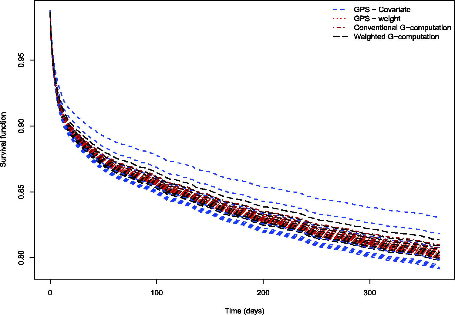

4. Monte Carlo simulations of the performance of the GPS for estimating the effect of continuous exposures on time-to-event outcomes

We conducted a series of Monte Carlo simulations to examine the performance of different methods of using the GPS to estimate the effect of continuous exposures on time-to-event outcomes. We used plasmode-type simulations in which the data-generating process was based on empirical analyses of the data described in the preceding section.¹⁵ We simulated data so that the distribution of baseline covariates resembled that of the EFFECT sample. Furthermore, we simulated a quantitative exposure variable so that its relationship with the confounding variables was similar to that observed above. Finally, we simulated a time-to-event outcome such that its association with the baseline covariates was informed by the analyses described above.

4.1 Methods

4.1.1 Simulating a large super-population

Using the data described in Section 3.1, we estimated the Pearson variance–covariance matrix for the 34 baseline covariates. We also determined the prevalence of each of the 23 binary covariates. Recall that the 11 continuous covariates had been standardized to have mean zero and unit variance.

We simulated baseline covariates for a large super-population consisting of 1,000,000 subjects. Thirty-four baseline covariates ( $X_{1} - X_{34}$ ) were simulated for each subject from a multivariate normal distribution with mean zero and variance–covariance matrix equal to that estimated above. The 11 covariates with mean zero and unit variance were retained as continuous covariates. The 23 remaining covariates were dichotomized to create binary variables whose prevalences were equal to the prevalences of the binary covariates analyzed above. This was done by categorizing each of the 23 covariates according to whether its value was above or below the appropriate quantile of the marginal normal distribution. The use of this process allowed us to simulate 34 baseline covariates whose multivariate distribution resembled that of the empirical data analyzed in Section 3.1.

For each subject in the large super-population, we then randomly generated a quantitative exposure variable. To do so, we first used the empirical EFFECT data to regress the standardized income variable on the 34 baseline covariates using OLS. The estimated vector of regression coefficients was extracted:

β_{income - EFFECT}

(see Table 1 for the estimated regression coefficients). Let

X_{baseline}

denote the matrix of simulated baseline covariates for the large super-population (consisting of 34 columns and 1,000,000 rows). Let

X_{B + I}

denote the previous matrix with an additional column added to denote the intercept (the first column of

X_{B + I}

consists of 1 s). We simulated a continuous exposure variable for each subject in the large super-population as:

Z \sim X_{B + I} β_{income - EFFECT} + ɛ, where ɛ \sim N (0, σ^{2})

. Thus the relationship between the continuous exposure and the 34 baseline covariates reflected that which was observed in the empirical analysis of the EFFECT data. The one modification that we made was that we selected the value of

σ^{2}

(the residual variance) in order to have a specific value of the model R². We use the model R² as a measure of the strength of confounding (the degree to which variation in the continuous exposure is explained by variation in the 34 baseline covariates). For a given value of R², we used a bisection approach to determine the appropriate value of

σ^{2}

. We considered six different values of R²: 0.1, 0.2, 0.3, 0.4, 0.5, and 0.6.

Table 1.

Regression coefficients for exposure model and outcomes model.

Covariate	Exposure (income) Model	Outcome (hazard) Model
Intercept (linear model for exposure)/ Income effect (hazard model for outcome)	0.071	−0.036
Age	0.037	0.846
Systolic blood pressure	−0.004	−0.352
Diastolic blood pressure	−0.002	−0.013
Heart rate	0.014	0.130
Respiratory rate	−0.053	0.129
Glucose	−0.002	0.148
White blood count	0.015	0.096
Hemoglobin	0.020	−0.108
Sodium	−0.004	−0.022
Potassium	0.009	0.091
Creatinine	−0.015	0.156
Female	−0.040	−0.012
Acute congestive heart failure	0.010	−0.034
Cardiogenic shock	−0.044	1.277
Diabetes	−0.102	0.123
Current smoker	−0.081	0.011
Stroke or transient ischemic attack	−0.025	0.137
Hyperlipidemia	0.111	−0.086
Hypertension	0.005	0.031
Family history of CAD	−0.011	−0.168
Angina	−0.079	0.118
Cancer	0.070	0.133
Dementia	0.137	0.254
Previous AMI	−0.047	0.077
Asthma	−0.075	−0.143
Depression	0.003	0.189
Hyperthyroidism	−0.142	0.035
Peptic ulcer disease	−0.033	−0.232
Peripheral vascular disease	−0.015	0.246
Previous coronary revascularization	0.036	0.078
History of bleeding	0.210	0.079
Chronic congestive heart failure	−0.020	0.233
Renal disease	0.190	−0.442
Aortic stenosis	−0.012	0.333

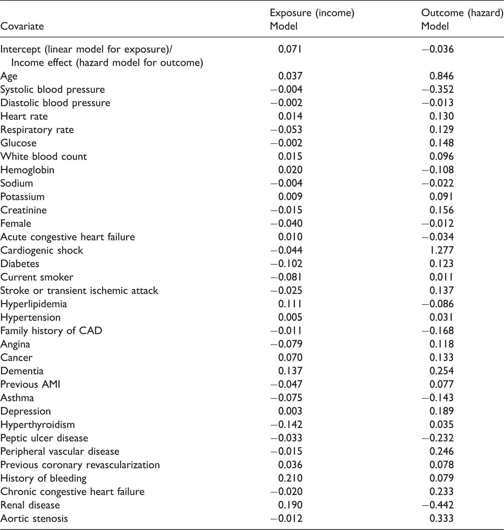
Note: The continuous covariates were standardized to have mean zero and unit variance. Thus, the regression coefficients denote the effect of a one standard deviation increase in the covariate on the mean exposure or the log-hazard of the outcome.

We simulated a time-to-event outcome for each subject so that the relationship between the hazard of the outcome and the 34 baseline covariates would be similar to what was observed in the EFFECT sample. First, using the EFFECT sample, we regressed the hazard of death on standardized neighbourhood income and the 34 baseline covariates using a Cox proportional hazards model. We denote the vector of estimated regression coefficients by $β_{hazard - EFFECT}$ (see Table 1 for the estimated regression coefficients). We then made one modification to this vector of regression coefficients: we changed the regression coefficient for standardized average income to log(15). This was done to induce greater separation in the dose–response functions. For a given subject in the large super-population, let $X_{Z + B}$ denote the vector consisting of the simulated continuous exposure variable (income) and the 34 baseline covariates, and let $X_{Z + B} β_{hazard - EFFECT}$ denote the corresponding linear predictor. Then, we used methods described by Bender et al. to simulate a time-to-event outcome from a Cox–Gompertz model: $T = \frac{1}{α} log [1 - \frac{α log (U)}{λ X_{Z + B} β_{hazard - EFFECT}}]$ , where $U \sim Uniform (0, 1)$ and α and λ denote the shape and scale parameter, respectively. In our simulations, we set the shape and scale parameters equal to 0.005 and 0.00005, respectively.

The above process allowed us to simulate 34 baseline covariates, a continuous exposure, and a time-to-event outcome for a large super-population so that: (i) the multivariate distribution of the 34 baseline covariates resembled that of the EFFECT data; (ii) the relationship between the continuous exposure and the 34 baseline covariates was similar to the relationship observed in the EFFECT data; (iii) the association between the hazard of the outcome and the 34 baseline covariates reflected that which was observed in the EFFECT data.

Let T₉₅ denote the 95th percentile of the simulated time-to-events in the large super-population. When determining the population dose–response function and sample estimates of the dose–response function, we will estimate the survival function for $t \leq T_{95}$ .

We then determined the population dose–response function at a pre-determined number of values of the continuous exposure variable. We computed the nine deciles of the population distribution of the continuous exposure. We refer to these nine deciles as the nine exposure thresholds. We then used methods identical to those described above to simulate a time-to-event outcome for each subject in the large super-population if everyone in the super-population had their exposure set equal to the first of the nine exposure threshold values. We then computed the Kaplan–Meier estimate of the survival function for the outcome in the super-population if all subjects were to receive the given level of exposure. This process was repeated for the other eight exposure thresholds values. These nine survival functions will serve as the population dose–response function. Thus the population dose–response function consisted of nine survival functions. Each survival function was equal to the population survival function if all members of the population were to receive that level of exposure.

4.1.2 Monte Carlo simulations

From the large super-population, we drew a random sample of 1000 subjects. In this random sample, we estimated the propensity function using OLS regression to regress the quantitative exposure variable on all 34 baseline covariates. The GPS was estimated under the assumption that the conditional distribution of the exposure was normal with mean equal to the linear predictor and with variance equal to the residual variance of the fitted OLS regression model. We then used the two methods described above for using the GPS to estimate the dose–response function for time-to-event outcomes. We estimated the dose–response function at the nine exposure threshold described above (the nine deciles of the population distribution of the continuous exposure). We compared the performance of the two methods based on the GPS with that of conventional G-computation and weighted G-computation.

The process of drawing random samples of size 1000 from the super-population was conducted 10,000 times. For each estimation method, we determined the mean dose–response function across the 10,000 iterations of the simulations. For each time at which the survival function was estimated and for a given method and for each of the nine exposure thresholds, we determined the standard deviation of the value of the dose–response function across the 10,000 iterations of the simulations.

We varied one factor in the Monte Carlo simulations: the proportion of the variation in the continuous exposure that was explained by variation in the 34 baseline covariates. We considered six values for this R²: 0.1, 0.2, 0.3, 0.4, 0.5, and 0.6. We thus constructed six different super-populations. From each super-population, we drew 10,000 random samples and conducted the statistical analyses described above. The magnitude of the R² statistic can be thought of as a measure of the magnitude of confounding. Higher values of R² are indicative of a greater correlation between the continuous exposure variable and a linear combination of the baseline covariates. Thus, we considered scenarios in which the magnitude of confounding ranges from weak to relatively strong.

4.2 Results

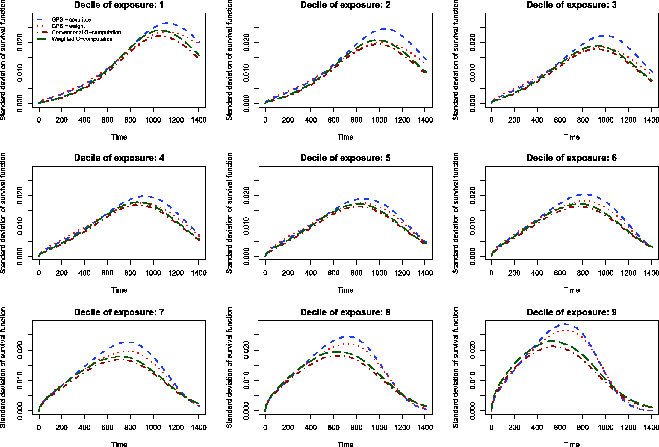
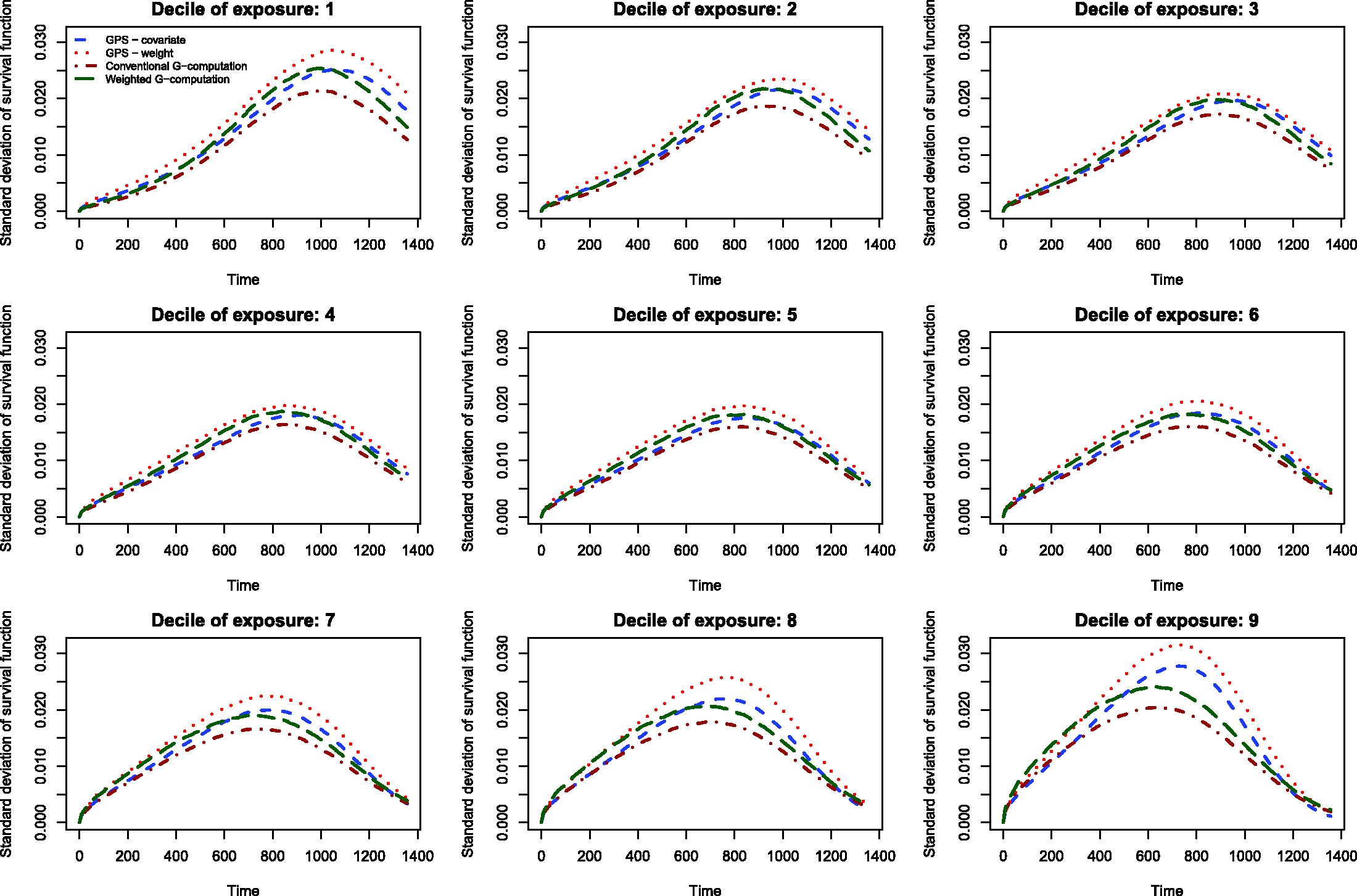
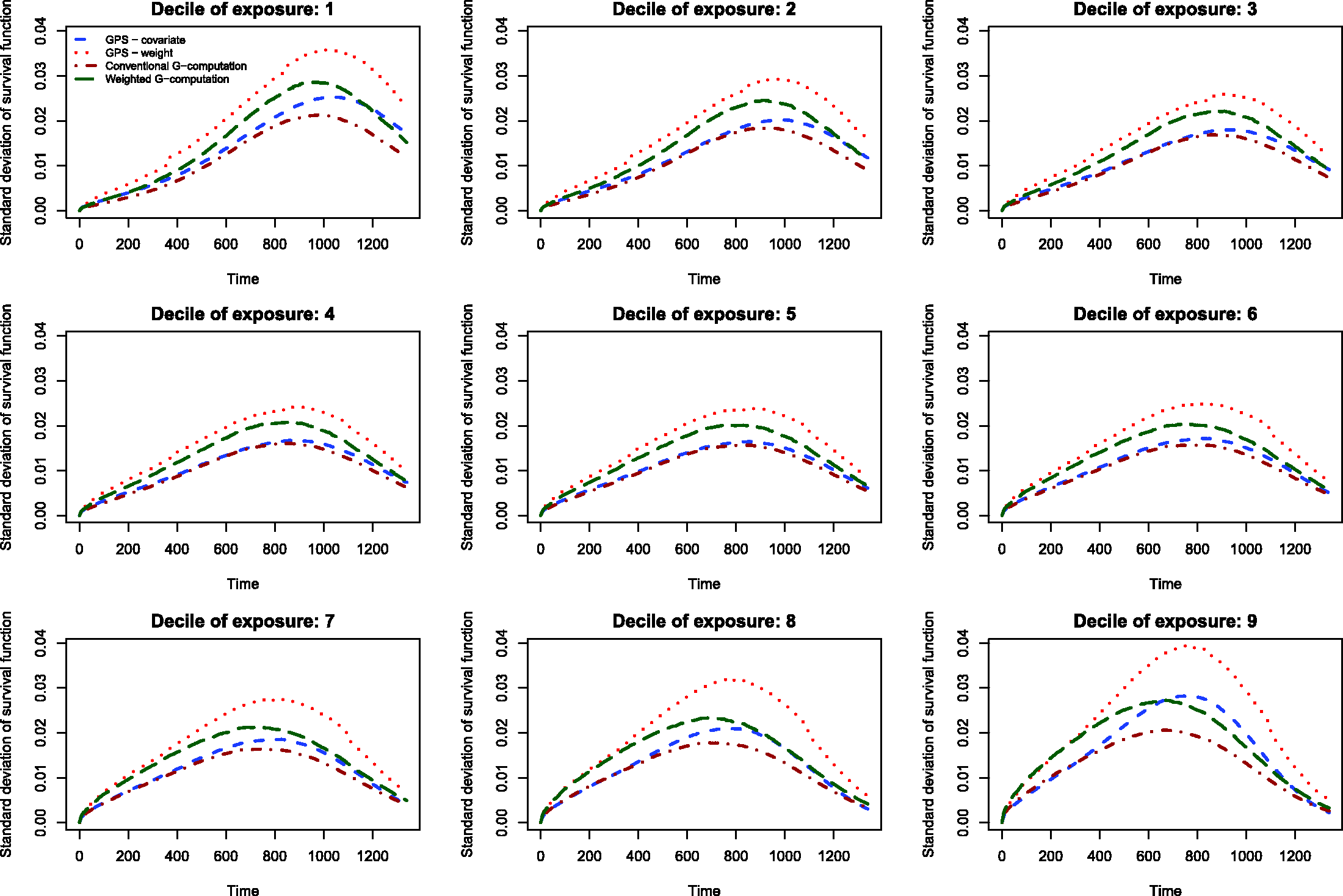
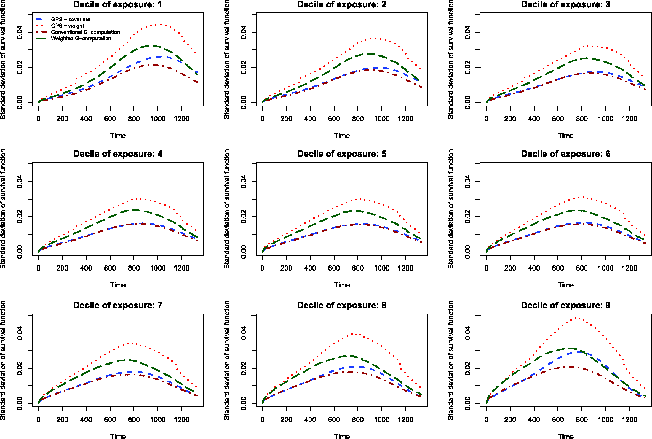
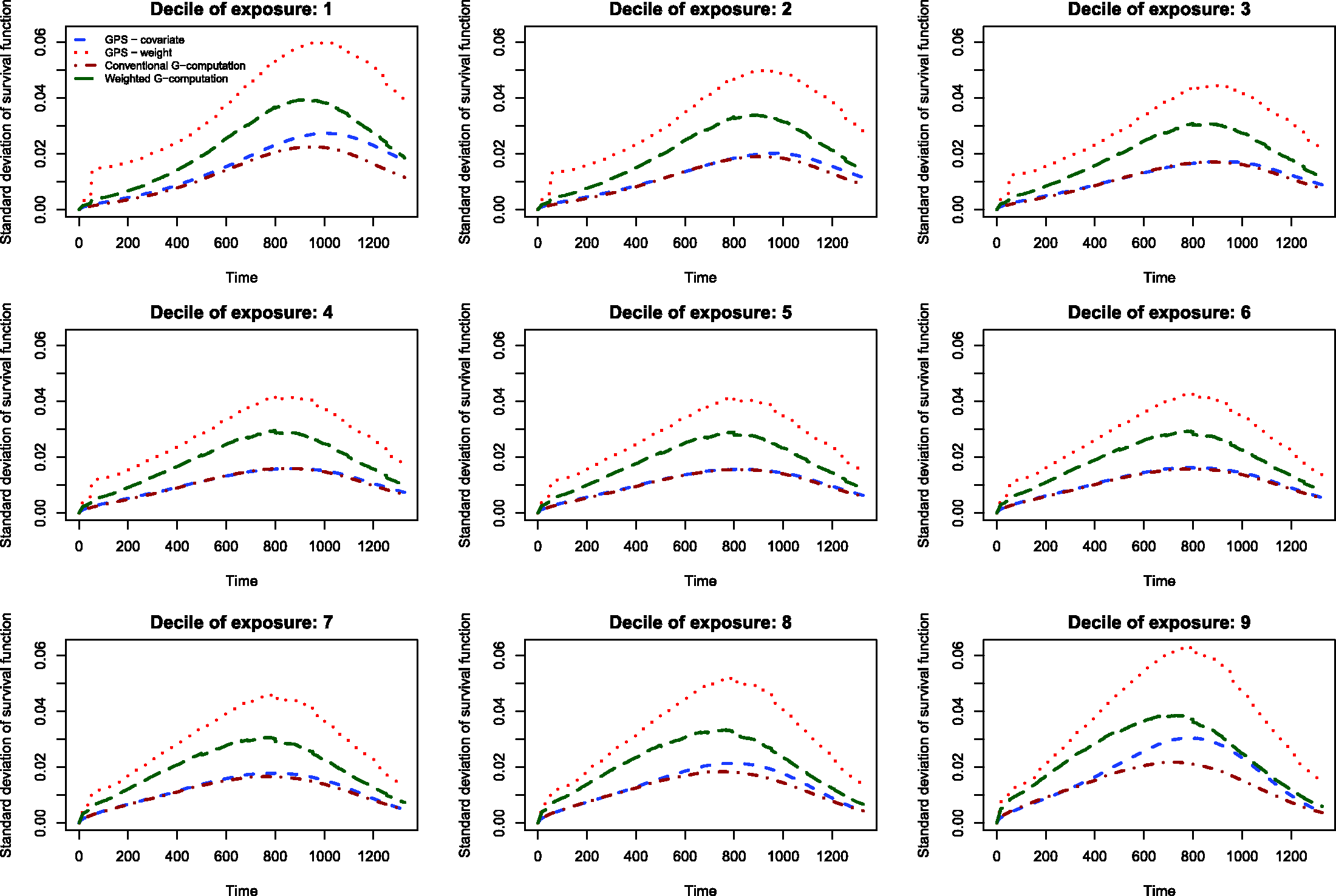
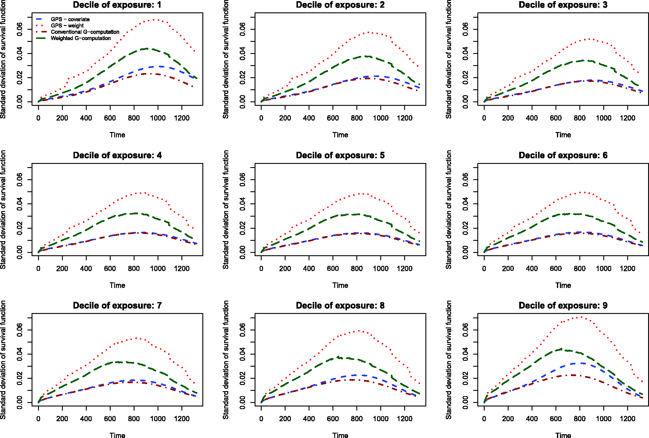
The results of the Monte Carlo simulations are reported in Figures 2 through 14. The population dose–response function and the mean estimated dose–response functions are reported in Figures 2 through 7, the average magnitude of the bias in estimating the dose–response functions is summarized in Figure 8, while the standard deviations of the estimated dose–response functions are described in Figures 9 through 14.

Figure 2.

Estimates of dose–response function when R²= 0.1.

Figure 3.

Estimates of dose–response function when R²= 0.2.

Figure 4.

Estimates of dose–response function when R²= 0.3.

Figure 5.

Estimates of dose–response function when R²= 0.4.

Figure 6.

Estimates of dose–response function when R²= 0.5.

Figure 7.

Estimates of dose–response function when R²= 0.6.

Figure 8.

Mean absolute difference between estimated survival curve and population survival curve.

Figure 9.

Standard deviation of dose–response function when R²= 0.1.

Figure 10.

Standard deviation of dose–response function when R²= 0.2.

Figure 11.

Standard deviation of dose–response function when R²= 0.3.

Figure 12.

Standard deviation of dose–response function when R²= 0.4.

Figure 13.

Standard deviation of dose–response function when R²= 0.5.

Figure 14.

Standard deviation of dose–response function when R²= 0.6.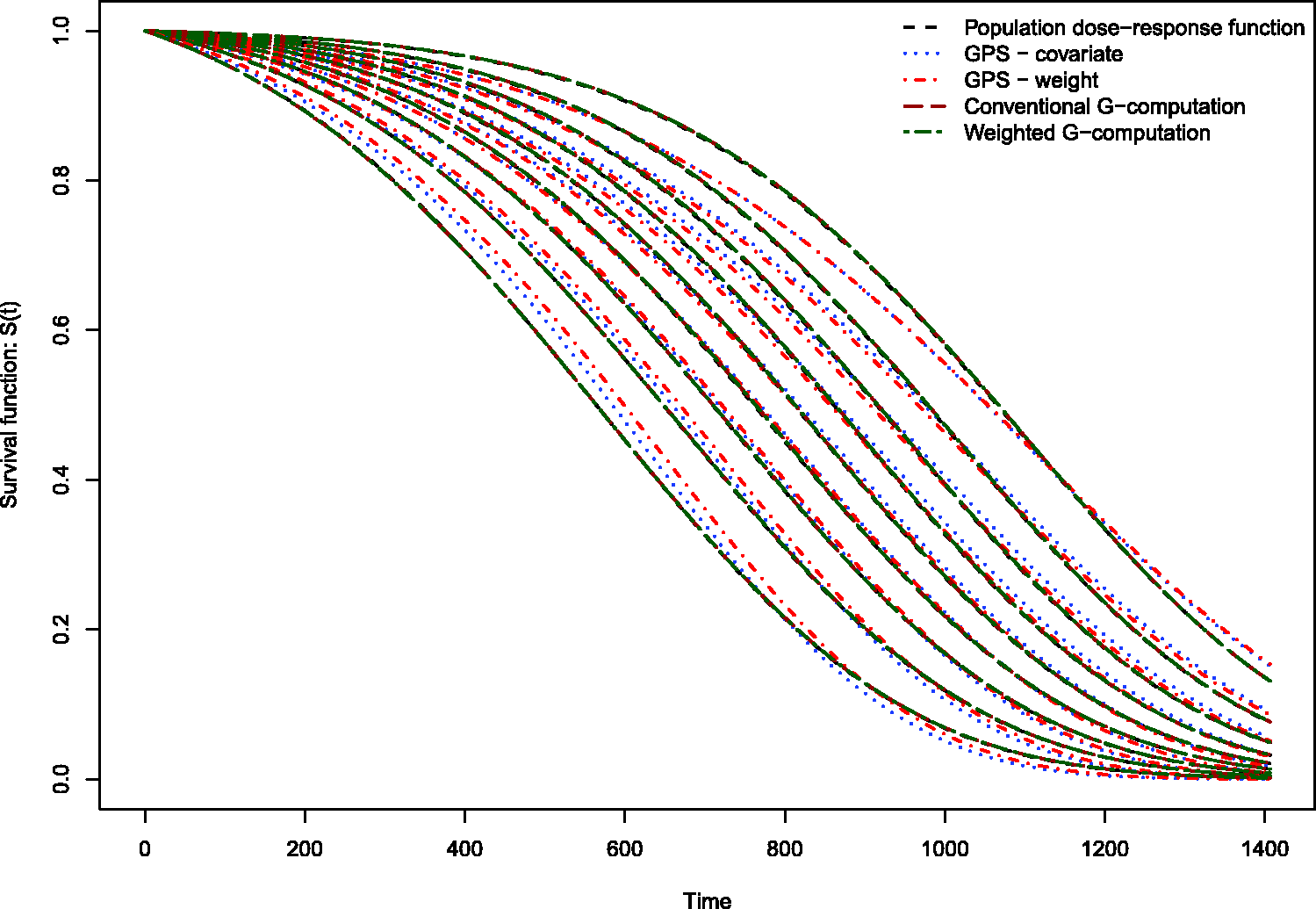

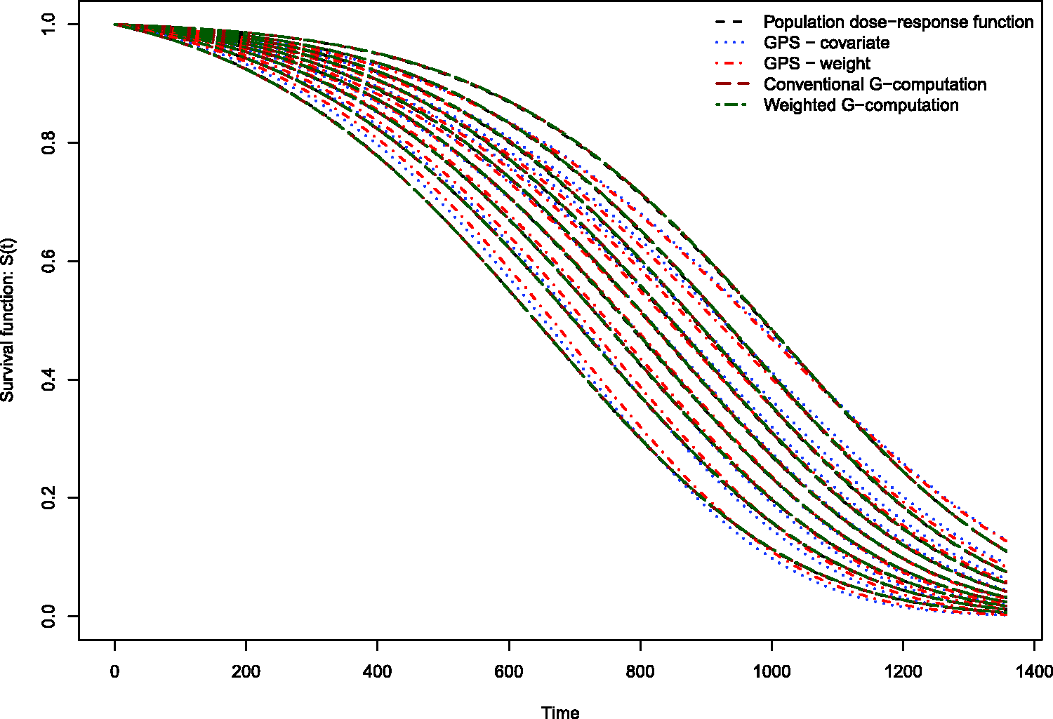
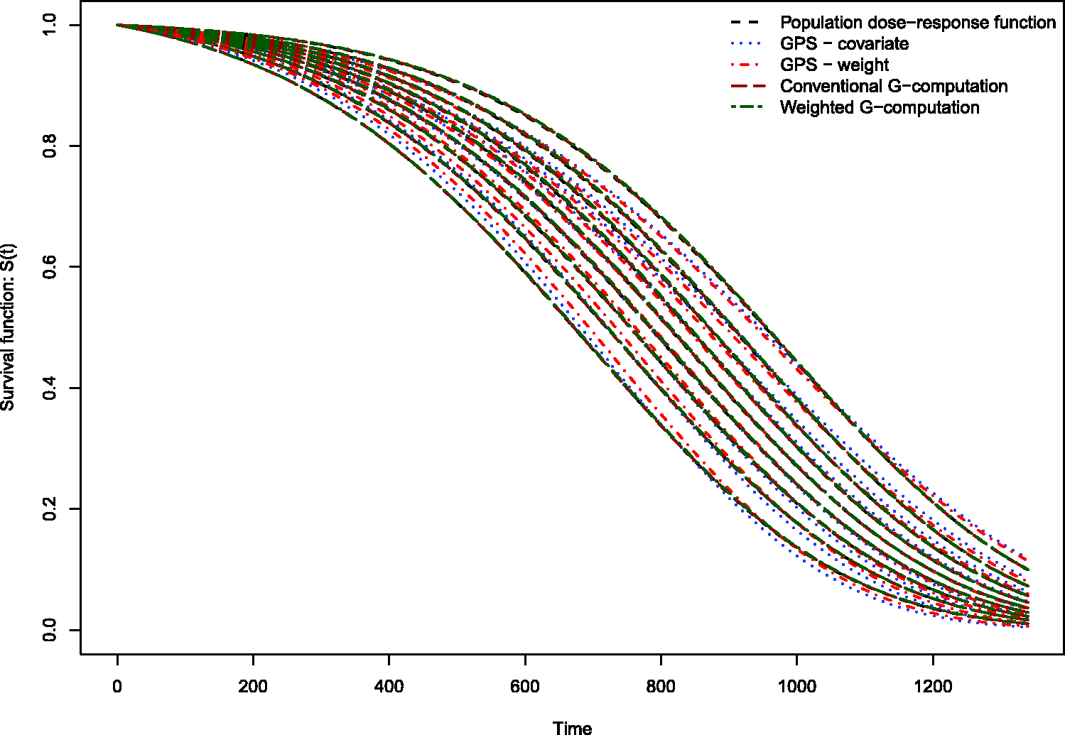
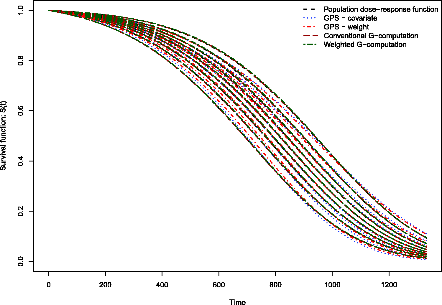
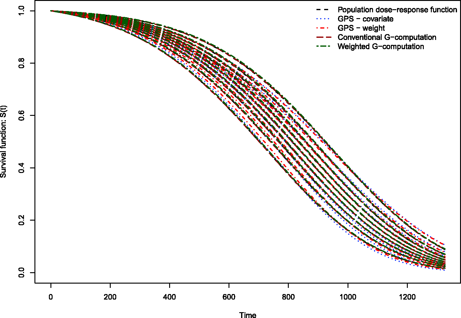
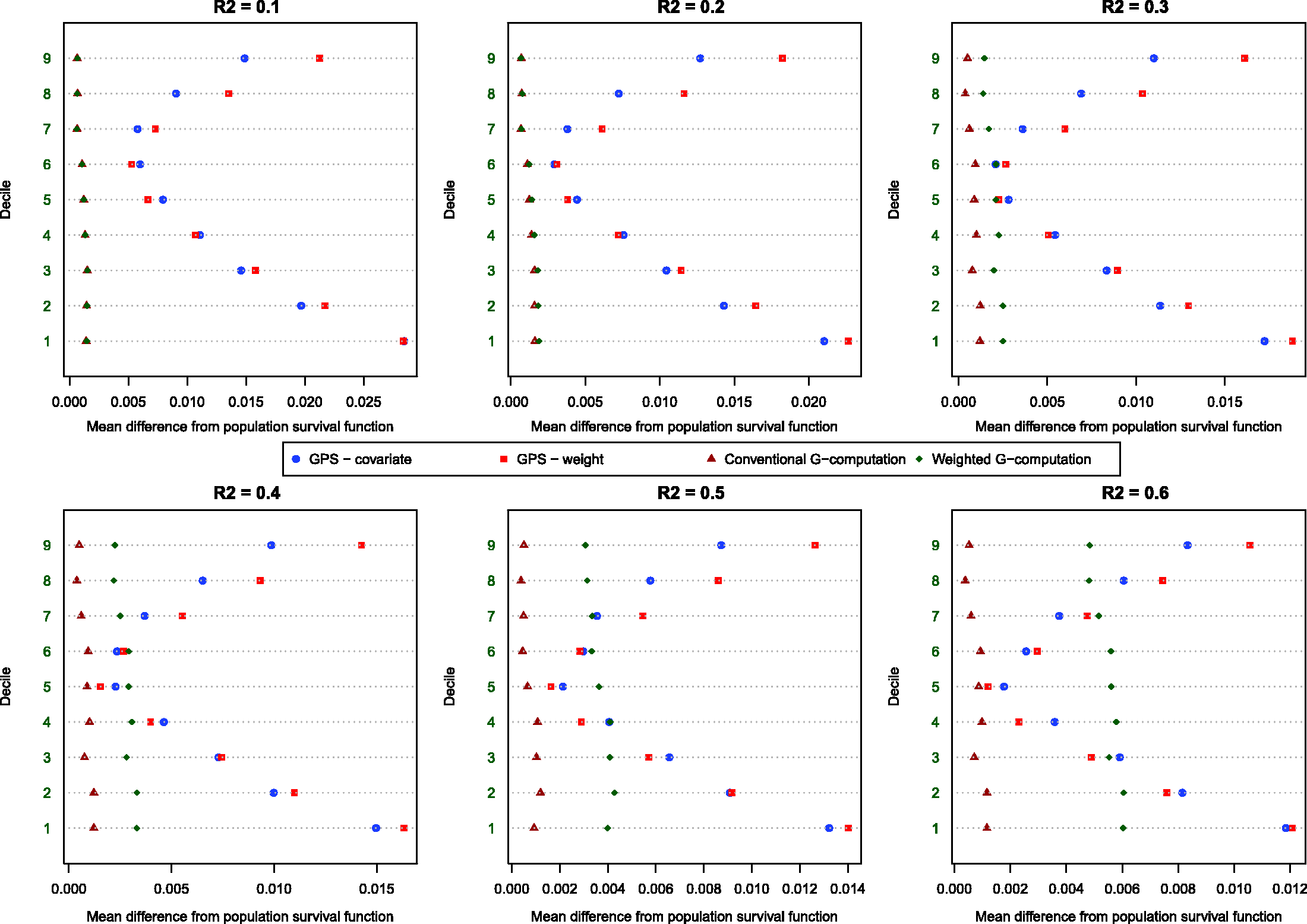
Conventional G-computation resulted in essentially unbiased estimates of the dose–response function across the six different scenarios (Figures 2 through 7). There is one figure for each of the different R² values. GPS-based methods for estimating the dose–response function resulted in marginal bias. The bias was largest when estimating the survival function associated with the more extreme deciles of the quantitative exposure. To summarize the magnitude of the bias in estimating the population dose–response function, we used numerical integration to compute the area between each estimated dose–response function and the population dose–response function. The magnitude of the average bias is summarized in Figure 8. Across all six scenarios, the mean difference between the population probability of an event and the estimated probability of an event was minimal when conventional G-computation was used. When R² was less than or equal to 0.4, weighted G-computation tended to result in the next lowest bias. When considering only the two GPS-based approaches, in general, covariate adjustment using the GPS tended to result in estimates with less bias than did weighting using stabilized GPS-based weights. However, in many instances the differences between the two methods was modest.

The standard deviations in estimating survival probabilities across the duration of follow-up time are reported in Figures 9 through 14. There is one figure for each of the R² values. Each figure consists of nine panels, one for each of the nine deciles of the quantitative exposure. For a given value of time, conventional G-computation tended to result in estimates that displayed the lowest variability. When the R² was 0.2 or greater, weighting using the GPS-based weights tended to result in estimates that displayed the greatest variability. As R² increased, the estimates obtained using covariate adjustment using the GPS displayed variability that was close to that observed when using conventional G-computation. This was particularly evident for the non-extreme deciles of the quantitative exposure.

5. Discussion

In the current study, we evaluated the performance of different methods of using the GPS to estimate the effect of quantitative exposures on survival or time-to-event outcomes. Covariate adjustment using the GPS and weighting using stabilized GPS-based weights tended to result in estimates with comparable bias. The bias tended to decrease as the magnitude of confounding increased. However, the use of conventional G-computation resulted in estimates with the lowest bias. Furthermore, conventional G-computation resulted in estimates that displayed the lowest variability.

As noted in section 1, the original methods papers that introduced the GPS considered continuous outcomes such as labor earnings,^5,6 medical expenditures,⁴ and birth weight.⁷ A recent paper examined the use of the GPS for estimating the effects of quantitative exposures on binary outcomes.¹⁶ In biomedical research, time-to-event outcomes occur frequently.⁸ Despite the frequency of time-to-event outcomes in epidemiological and medical research, there is a paucity of studies examining the performance of the GPS for estimating the effect of continuous or quantitative exposures on time-to-event outcomes. The current study addresses this void in the methodological literature.

In the current study, the primary focus has been on using the GPS to estimate the survival function conditional on a specific value of the quantitative exposure. In some settings, the primary interest may be in estimating treatment effects between two different levels of the quantitative exposure. In such a setting, one would estimate the two survival functions associated with the two different exposure levels. The difference in the two survival curves can then be computed. Pointwise 95% confidence intervals for the difference in survival can be computed using bootstrap methods. Frequently, one may be interested in survival differences at a fixed point in time (e.g. one year). If that is the case, one can simply estimate the probability of survival until the fixed time point under each of the two exposure levels and then compute the difference in these two survival probabilities. Bootstrap methods can be used to compute a 95% confidence interval.

In the current study, we observed that conventional G-computation tended to result in estimates that displayed both the lowest bias and the lowest variability. In interpreting the results of the simulations, it is important to remember that G-computation requires the specification of an outcomes model in which the outcome is related to both exposure and the baseline covariates. In our simulations, the G-computation method used a correctly specified outcomes model. In particular, it used the model that was used to generate outcomes in the large super-population. Thus, it is not surprising that G-computation had the best performance. Indeed, one could argue that it would have been surprising had it not had the best performance. While our simulations suggest that conventional G-computation is an attractive analytic option, it requires that an outcomes model be correctly specified. In practice, it is difficult to ascertain whether a multivariable outcomes model has been correctly specified. In contrast to this, a variety of balance diagnostics have been proposed for use with the GPS.^5,6,17 These allow one to assess whether incorporating the GPS has allowed one to balance the distribution of measured baseline covariates between subjects with different values of the continuous exposure. Thus, from an implementation perspective, the use of GPS-based methods is appealing. In practice, the potential for decreased bias and variability must be balanced with the potential to ascertain whether adequate covariate balance has been achieved. A further limitation to the use of G-computation is that when the outcome is rare, an inadequate number of events may have occurred to permit adequate regression adjustment. For instance, Peduzzi et al. suggest that a minimum of 10 events be observed for each variable entered in a Cox regression model.¹⁸ In small samples or when outcomes are rare, there may be an insufficient number of observed outcomes to permit inclusion of all of the desired covariates in the model to account for measured confounding. In contrast to this, estimation of the propensity function can often be done using OLS regression, which requires a much lower number of subjects per variable.¹⁹ Thus, the use of GPS-based methods may allow for accounting for imbalance in a larger number of baseline covariates than does G-computation.

Our use of weighted G-computation is similar to the weighted regression estimator proposed by Zhang et al. for use with quantitative exposures.⁷ Their estimator was for use in the context when one was estimating the expected outcome under different values of the quantitative exposure. Thus, it is most readily applicable to settings with continuous or binary outcomes (indeed, in their case study, the outcome is an infant’s birth weight – a continuous outcome). Under certain conditions, their weighted regression estimator has doubly-robust properties. In the current study, we found that weighted G-computation had inferior performance compared to conventional G-estimation when estimating expected survival curves. The reasons for this poor performance merit study in future research.

There are certain limitations to the current study. The primary limitation is that the evaluation of the performance of different methods of using the GPS to estimate the effect of continuous exposures on time-to-event outcomes was conducted using Monte Carlo simulations. However, we used a plasmode-type simulation so that the simulations would result in simulated datasets that resembled real-life data. Thus, the simulations have face validity, as they reflect a specific empirical dataset. However, it is possible that results would differ under different data-generating processes.

In summary, the current study represents the first study to examine the performance of different methods of using the GPS to estimate the effect of quantitative or continuous exposures on survival or time-to-event outcomes. We found that both covariate adjustment using the GPS and weighting using stabilized GPS-based weights resulted in estimates of the dose–response function with at most modest bias. However, the use of conventional G-computation resulted in estimates with the lowest bias and that displayed the lowest variability.

Footnotes

Declaration of conflicting interests

The author(s) declared no potential conflicts of interest with respect to the research, authorship, and/or publication of this article.

Funding

The author(s) disclosed receipt of the following financial support for the research, authorship, and/or publication of this article: This study was supported by the Institute for Clinical Evaluative Sciences (ICES), which is funded by an annual grant from the Ontario Ministry of Health and Long-Term Care (MOHLTC). The opinions, results and conclusions reported in this paper are those of the authors and are independent from the funding sources. No endorsement by ICES or the Ontario MOHLTC is intended or should be inferred. This research was supported by an operating grant from the Canadian Institutes of Health Research (CIHR) (MOP 86508) and by the National Institutes of Health (NIH)/National Heart, Lung, and Blood Institute (NHLBI) (Grant Number: 1 R01 HL130484-01A1). Dr Austin was supported by Career Investigator awards from the Heart and Stroke Foundation. This study was approved by the institutional review board at Sunnybrook Health Sciences Centre, Toronto, Canada. These datasets were linked using unique encoded identifiers and analyzed at the Institute for Clinical Evaluative Sciences (ICES). The Enhanced Feedback for Effective Cardiac Treatment (EFFECT) data used in the study was funded by a CIHR Team Grant in Cardiovascular Outcomes Research (grant numbers CTP 79847 and CRT43823).

References

Rosenbaum

Rubin

. The central role of the propensity score in observational studies for causal effects. Biometrika 1983; 70: 41–55.

Austin

. An introduction to propensity-score methods for reducing the effects of confounding in observational studies. Multivariate Behav Res 2011; 46: 399–424.

Imbens

. The role of the propensity score in estimating dose–response functions. Biometrika 2000; 87: 706–710.

Imai

van Dyk

. Causal inference with general treatment regimes: generalizing the propensity score. J Am Stat Assoc 2004; 99: 854–866.

Hirano K and Imbens GW. The propensity score with continuous treatments. In: Gelman A and Meng X-L (eds) Applied Bayesian modeling and causal inference from incomplete-data perspectives. Chichester: John Wiley & Sons, Ltd, 2004, pp.73–84.

Bia

Mattei

. A Stata package for the estimation of the dose–response function through adjustment for the generalized propensity score. Stata J 2008; 8: 354–373.

Zhang

Zhou

Cao

, et al. Causal inference with a quantitative exposure. Stat Meth Med Res 2016; 25: 315–335.

Austin

Manca

Zwarenstein

, et al. A substantial and confusing variation exists in handling of baseline covariates in randomized controlled trials: a review of trials published in leading medical journals. J Clin Epidemiol 2010; 63: 142–153.

Robins

Hernan

Brumback

. Marginal structural models and causal inference in epidemiology. Epidemiology 2000; 11: 550–560.

10.

McCullagh

Nelder

. Generalized linear models, London: Chapman & Hall, 1989.

11.

Yang

Joffe

Hennessy

, et al. Covariance adjustment on propensity parameters for continuous treatment in linear models. Stat Med 2014; 33: 4577–4589.

12.

Therneau

Grambsch

. Modeling survival data: extending the Cox model, New York, NY: Springer-Verlag, 2000.

13.

Donovan

Lee

, et al. Effectiveness of public report cards for improving the quality of cardiac care: the EFFECT study: a randomized trial. J Am Med Assoc 2009; 302: 2330–2337.

14.

Snowden

Rose

Mortimer

. Implementation of G-computation on a simulated data set: demonstration of a causal inference technique. Am J Epidemiol 2011; 173: 731–738.

15.

Franklin

Schneeweiss

Polinski

, et al. Plasmode simulation for the evaluation of pharmacoepidemiologic methods in complex healthcare databases. Comput Stat Data Anal 2014; 72: 219–226.

16.

Austin PC. Assessing the performance of the generalized propensity score for estimating the effect of quantitative or continuous exposures on binary outcomes. Stat Med 2018; 37: 1874–1894.

17.

Austin

. Assessing covariate balance when using the generalized propensity score with quantitative or continuous treatments. Stat Meth Med Res 2017; 28: 1365–1377.

18.

Peduzzi

Concato

Feinstein

, et al. Importance of events per independent variable in proportional hazards regression analysis. II. Accuracy and precision of regression estimates. J Clin Epidemiol 1995; 48: 1503–1510.

19.

Austin

Steyerberg

. The number of subjects per variable required in linear regression analyses. J Clin Epidemiol 2015; 68: 627–636.

Assessing the performance of the generalized propensity score for estimating the effect of quantitative or continuous exposures on survival or time-to-event outcomes

Abstract

Keywords

1 Introduction

2 Using the generalized propensity score with time-to-event outcomes

2.1 The generalized propensity score

2.2 Estimation of the dose–response function using the generalized propensity score

3 Case study

3.1 Data and analyses

3.2 Results

4. Monte Carlo simulations of the performance of the GPS for estimating the effect of continuous exposures on time-to-event outcomes

4.1 Methods

4.1.1 Simulating a large super-population

4.1.2 Monte Carlo simulations

4.2 Results

5. Discussion

Footnotes

Declaration of conflicting interests

Funding

References