Sage Journals: Discover world-class research

Abstract

In this article, I provide an overview of existing community-contributed commands for executing event studies. I assess which command could have been used to conduct event studies that have appeared in the past 10 years in 3 leading accounting, finance, and management journals. The older command eventstudy provides a comfortable graphical user interface and good functionality for event studies that do not require hypotheses testing. The command estudy, described in Pacicco, Vena, and Venegoni (2018, Stata Journal 18: 461–476; 2021, Stata Journal 21: 141–151), provides a set of commonly applied test statistics and useful exporting routines to spreadsheet software and LAT_EX for event studies with a limited number of events. The most complete command in terms of available test statistics and benchmark models as well as its ability to handle events with insufficient data, thin trading, and large samples is eventstudy2.

Keywords

st0643 event studies estudy eventstudy eventstudy2

1 Introduction

Event studies represent a standardized method to measure and statistically assess stock price reactions to unanticipated events. For instance, Ball and Brown (1968) use this method to show that earnings surprises move stock prices. Fama et al. (1969) show that stock splits have a positive average impact on stock prices. Since the publication of these two seminal articles, event studies have become a workhorse method whenever researchers want to test whether any news event has an impact on stock prices. The scenarios range from dividend announcements (for example, Asquith and Mullins [1983]; Kane, Lee, and Marcus [1984]), mergers and acquisitions (for example, Capron and Pistre [2002]; Halpern [1983]), and changes in legislation and corporate litigation (for an overview, see Bhagat and Romano [2002a]; Bhagat and Romano [2002b]) to celebrity endorsement of products (for example, Agrawal and Kamakura [1995]), nuclear catastrophes (for example, Bowen, Castanias, and Daley [1983]; Hill and Schneeweis [1983]), and hurricanes (for example, Lamb [1998]).

In the past decades, several software solutions for conducting event studies have emerged, most notably the SAS^®-based Eventus^® software, which has been directly embedded into the Wharton Research Data Services (WRDS) platform and thus has become a gold standard for event studies that focus on U.S. firms. Nevertheless, probably because only top-ranked universities and other top research institutions have access to WRDS and Eventus, free event-study software packages in other programming environments (for example, R and Python) have become available. Also, Stata users can currently draw on three different community-contributed commands (in chronological order of their first appearance on the Statistical Software Components archive of the Boston College Department of Economics):

eventstudy (Zhang, Li, and Xu 2013)

eventstudy2 (Kaspereit 2015, updated November 2019)

estudy (Pacicco, Vena, and Venegoni 2018, 2019, 2021)

In this article, I analyze which of the three commands is suitable for which type of event study. My analysis reveals that the chronological order of appearance does not represent stages of evolution. Instead, each command is applicable to different types and tasks within the universe of event-study designs or has certain features that make it more or less suitable for specific types and tasks. The older command eventstudy provides a comfortable graphical user interface (GUI) and good functionality for event studies that do not require hypotheses testing. The command estudy provides a set of commonly applied test statistics and useful exporting routines to spreadsheet software and L^AT_EX. The most complete command in terms of available test statistics and benchmark models as well as its ability to handle events with insufficient data, thin trading, and large samples is eventstudy2.

My analysis is based on three pillars. First, I identify the conceptual characteristics of event studies. Instead of reiterating the statistical fundamentals of the event-study method, which have already been presented elsewhere (for example, Corrado [2011]; Kothari and Warner [2007]; MacKinlay [1997]), I focus on what conceptually constitutes an event study, that is, what researchers are aiming for when using this research design, and whether or how the three community-contributed commands meet these user demands. Second, I back my assertions by analyzing all event studies that have been published in three leading field journals: the Journal of Accounting Research, the Journal of Finance, and Management Science, during the period 2009–2018. Third, I assess the practical features and limitations of the three commands with respect to run time, consistency, and handling of thinly traded stocks.

My analysis does not focus on input and output routines because their usefulness is in the eye of the beholder, while test statistics, benchmark models, maximum sample sizes, and run times are established features. Note, though, that in my opinion the oldest command, eventstudy, scores highest in the domain of data input because it is the only command that provides a GUI. In the domain of input data, eventstudy2 is the most complex command because it requires multiple .dta files (one for the event list, one for the security returns, and one for the market or factor returns). On the one hand, it will potentially take longer for the user to fully understand it. On the other hand, this data-input scheme is consistent with the data-delivery formats of popular financial data providers such as the Center for Research in Security Prices (CRSP), the Institutional Brokers’ Estimate System, and Compustat. The estudy command has the most comfortable output routines, including export to spreadsheet software and L^AT_EX.

2 Conceptual characteristics of event studies and community-contributed commands

2.1 Elements of event studies

In this section, I outline my framework of the three core elements, three supplemental elements, and two overarching principles of event studies, which will allow me to evaluate which of the three community-contributed event-study commands are most suitable for which empirical setting. In this framework (see table 1), the event leads the ranking of core elements because researchers are typically interested in measuring the impact of a specific event type on stock prices, for example, earnings announcements, stock splits, or dividend cuts. The firm and the event date (time) have to be properly identified but pose a methodological challenge rather than being at the center of the research.

Table 1.

Elements and principles of event studies

Core elements	Supplemental elements	Overarching principles
1. Event(s)	· Macroeconomic confounding event(s)	· Aggregation
2. Firms(s)	· Firm-specific confounding event(s)	· Synchronization
3. Time	· Statistical hypotheses testing

Because firms per se are not important and the focus is on the event, stock price reactions are aggregated across firms to eliminate random variation in returns not associated with the event. This corresponds to the overarching principle of aggregation (Corrado 2011, 212). Nevertheless, the firm ranks second in my list of core elements because many event studies aim at identifying how the impact of an event depends on firm characteristics, for example, firm size, magnitude of earnings surprise (Collins and Kothari 1989), or audit quality (Teoh and Wong 1993). In fact, as my analysis in the next section will show, these cross-sectional type of studies constitute a majority (97 out of 180 sample articles). Firms as individual objects, however, are rarely the object of research interest, and stock price reactions are either measured on an aggregated basis or hypothesized to be in a functional (linear) relationship with firm characteristics.

Time ranks third because researchers are typically not interested in whether an event has an impact on stock prices on a particular calendar day. For instance, it is unlikely that a researcher wants to analyze whether a stock split affects stock prices differently when announced on March 3 compared with September 15. In fact, the event-study method invokes the concept of event time, which is a timeline relative to the event day. For instance, if a similar event took place for Firm A on March 3 and Firm B on September 15, calendar days March 2, 3, and 4 and September 14, 15, and 16 are redefined as days [−1], [0], and [+1], respectively. Thus, the researcher’s or his or her software’s first and very important task is to rearrange the stock return data and put them onto a common timeline that is relative to the event dates. This corresponds to the overarching principle of synchronization.

The event-study method distinguishes itself from a simple examination of stock returns by properly addressing the problem of confounding events and by defining test statistics (statistical hypotheses testing) that address various econometric issues. Confounding events are events other than the event of research interest that potentially impact stock prices. They can be of macroeconomic (affecting all firms to some extent) or firm-specific (presumably affecting only one firm) character. The event-study method is well designed to eliminate the impact of macroeconomic events without significant loss of observations. By calculating and assessing abnormal return relative to a market index or multiple-factor model, researchers can effectively address the effect of overall market movements on event firms’ stock returns (MacKinlay 1997, 17–20). For instance, researchers can effectively address the effects of unanticipated changes in interest rates or terrorist attacks without even identifying these events. However, the event study method is incapable of addressing firm-specific confounding events. Those have to be identified by the researcher and taken into account by modifying the sample selection, potentially leading to some loss of observations.

2.2 Software requirements

From the above-described elements of event studies, several desirable features of eventstudy software solutions can be derived. They should assist the user in transforming the event and stock return data from common databases such as WRDS/CRSP, Datastream, or Yahoo! Finance from calendar time to event time. To that end, the command should, based on a common stock identifier and a date variable, merge a list of events with a dataset of stock returns. It should then rearrange the data to achieve an event-time structure with the date variable taking a value of zero at the event date (synchronization). This data management task is very important because it can be very time consuming and prone to error if executed manually using spreadsheet software.

The second core task any complete event-study software can perform is the calculation of abnormal returns against a benchmark model. Standard benchmark models are the constant mean return (COMEAN) model, the market model with a single market index as benchmark, and factor models such as the Fama and French (1993) three-factor model. Further, the software should be capable of calculating cumulative average abnormal returns (CAARs) and buy-and-hold average abnormal returns (Barber and Lyon 1997).

The third feature an event-study software should have is the implementation of statistical testing to assess (cumulative) average abnormal returns against the null hypothesis of them being zero. In fact, most of the methodological literature on event studies centers on the specification and empirical power of different parametric and nonparametric test statistics such as the crude dependence-adjustment t test by Brown and Warner (1980, 1985), the Patell (1976) Z statistic, the Corrado (1989) rank test, the Boehmer, Musumeci, and Poulsen (1991) parametric test with correction for event-induced volatility changes, the Kolari and Pynnönen (2010) adjustment of the Boehmer, Musumeci, and Poulsen (1991) test for cross-correlation, and the generalized rank (GRANK) test for CAARs (Kolari and Pynnönen 2011).

The fourth desirable feature of an event-study software package is its ability to present results and other output. Test statistics and statistical significance level should be tabulated alongside (cumulative) average abnormal returns. Further, a graphical presentation of CAARs is desirable because this is a standard presentation format in journal articles. The event-study software should report on events that had to be excluded and the reasons for their exclusion. Cumulative abnormal returns (CARs) should be made available for cross-sectional analysis.

2.3 Features of community-contributed commands

Table 2 summarizes the features of the three community-contributed commands. Although eventstudy and eventstudy2 do not share any programming code, the latter can be considered a substantial extension of the former. While eventstudy and eventstudy2 share the capability to synchronize data onto a common timeline that is relative to the events, eventstudy is restricted to the single-factor model to calculate abnormal returns. eventstudy does not provide any hypothesis testing capabilities, while eventstudy2 provides plenty. However, eventstudy provides a GUI, which the other two commands are lacking. Thus, eventstudy can be used if researchers are exclusively interested in calculating CARs and are not interested in assessing statistical significance or plan to assess statistical significance using their own routines. Although most of the methodological literature on event studies focuses on statistical hypotheses testing, the analysis of journal publications in the next section reveals that some studies do not apply these tests but are interested only in factors that explain abnormal returns. Therefore, the command eventstudy maintains its raison d’etre by being useful to researchers who can preserve run time by applying this less complex command.

Table 2.

Features of community-contributed event-study commands

Feature↓ \|\| Command→	eventstudy	eventstudy2	estudy
Data management (Synchronization)	yes	yes	Yes- Is able to use prices instead of returns
Calculation of abnormal returns (Benchmark model)	- Market model	- Market model- Raw returns- Constant mean returns- Market adjusted returns- Factor model (up to 12 factors)- Factor model with (G)ARCH- Buy-and-hold raw returns- Buy-and-hold abnormal returns	- Market model- Raw returns- Constant mean returns- Market adjusted returns- Factor model (up to maxvar)
Hypothesis testing (Test statistics)		- t test(assuming independence)- t test(crude adjustment)- Patell Z statistic- Adjusted Patell statistic- Boehmer–Musumeci–Poulsen test- Kolari and Pynnönen test- Generalized sign test- Wilcoxon signed-ranks test- Corrado rank test- Corrado and Zivney rank test- GRANK test- Bootstrapped t ratio	- t test(assuming independence)- Patell Z statistic- Adjusted Patell statistic- Boehmer–Musumeci– Poulsen test- Kolari and Pynnönen test- Wilcoxon signed-ranks test- GRANK test
Presentation (Tabulating abnormal returns; reporting on dropped observations)	- (Cumulative) abnormal returns are available for cross-sectional testing	- Tabulation ofaverage abnormal returns and significance levels- Tabulation of cumulative average abnormal returns and significance levels- Comprehensive reporting on dropped events- Graphical display of cumulative average abormal returns- (Cumulative) abnormal returns are available for cross-sectional testing	- Tabulation of cumulative (average) abnormal returns and significance levels- Graphical display of cumulative average abormal returns- (Cumulative) abnormal returns are available for cross-sectional testing- L^AT_EX-formatted output tables- Excel output of results

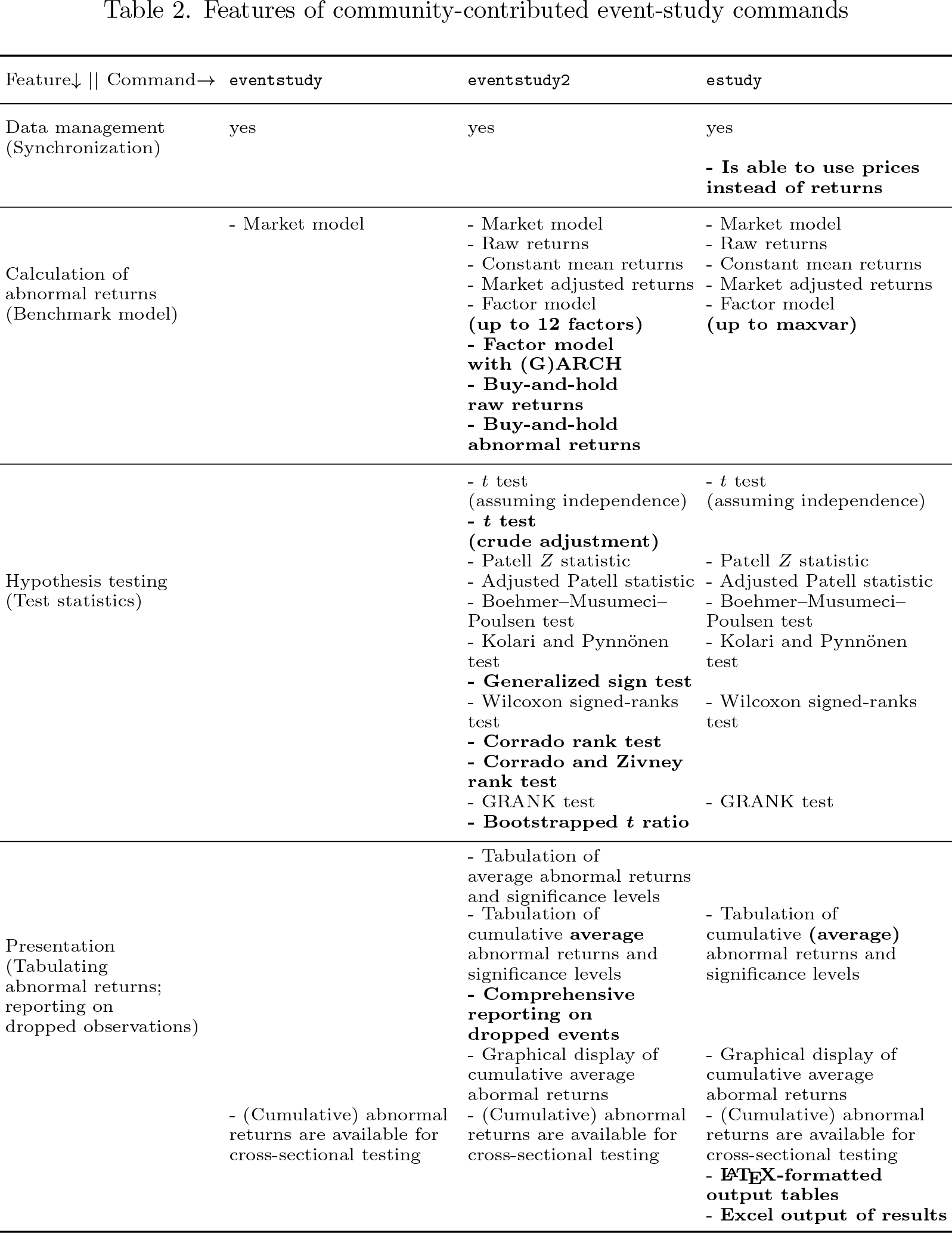
Table 2 also presents the differences in features of eventstudy2 and estudy. Because Pacicco, Vena, and Venegoni (2018, 461) state that their estudy command “significantly improves the existing commands in terms of both completeness and user comprehension,” with reference to eventstudy2, these differences are highlighted by bold fonts. Because estudy‘s data input is organized in wide rather than long format, it allows approximately as many factors to be included in the benchmark model as the respective Stata version can take variables. It is well known in the literature that one factor, the market index, or at most up to five factors (Fama and French 2015) add some explanatory power to the benchmark model. In fact, it is commonly known that the incremental effect on explanatory power is minor for all factors beyond the market index (MacKinlay 1997, 18). On the other hand, the wide-input data format of estudy imposes a restriction on the number of events. Pacicco, Vena, and Venegoni (2021, 3–4) state that their command can execute event studies with more than 24,000 companies. According to the outcomes of my tests of the estudy command, this limit applies not only to the number of companies but also to the number of events. It is important to understand that 24,000 companies would not impose a strong limitation because, even in big markets such as the U.S., samples rarely consist of more than 24,000 distinct companies. However, there are many studies that operate with samples of fewer companies but considerably more events (for example, Bhojraj et al. [2009]; Hail, Tahoun, and Wang [2014]; Savor and Wilson [2016]).

The estudy command provides output and statistical hypothesis testing by event firms, which eventstudy2 does not. However, researchers very rarely report abnormal returns and their statistical significance for each event firm separately because this would stand against the main idea of event studies of measuring the general effect of a specific type of event on firms, which corresponds to the above derived principle of aggregation (see table 1). The event ranks first, the firm only second. In fact, the very fundamental idea of event studies is to measure the average impact of an event type on stock returns. This calls for aggregation of abnormal returns and allows the application of the law of large numbers to arrive at lower standard errors in hypothesis testing (Corrado 2011; MacKinlay 1997).

eventstudy2 can calculate buy-and-hold abnormal returns and the respective bootstrapped t-ratio test statistic. It allows for different benchmarks for different event firms, which make the calculation of abnormal returns against characteristic-based benchmarks (Daniel et al. 1997), a method commonly used in finance and accounting research (for example, Da, Engelberg, and Gao [2011]), possible. It also reports on dropped observations or how it treats missing return observations, while the other two commands are lacking these features.

To conclude my conceptual comparison of the three community-contributed commands, I clearly see the relative merits of the eventstudy command if a researcher is interested in calculating only abnormal returns against the market model. eventstudy has a simple structure, which includes the most important data management tasks, and has a GUI that is most useful for inexperienced Stata users. eventstudy2 is the most complete command and provides comprehensive data management routines, hypothesis testing, and output. estudy is a useful command for studies with a limited number of events or if the researcher is interested in assessing the statistical significance of abnormal returns around the individual events. estudy is the only command that provides export routines to spreadsheet software and L^AT_EX.

3 Applicability to event studies in leading field journals

To substantiate my analysis of the usefulness of the three community-contributed eventstudy commands, I collect and analyze all studies that appeared between 2009 and 2018 in the Journal of Finance, Journal of Accounting Research, and Management Science and show which applied the event-study method either as their main method of analysis or as a tool to calculate abnormal returns for other purposes, for example, control variables.¹ The analysis in total comprises 180 articles, of which 55 appeared in the Journal of Accounting Research (17.5% of all articles that appeared in this journal during that period); 71 in the Journal of Finance (10.1%); and 54 in Management Science (3.0%). Thus, the event-study design can be considered one of the most prominent research methods in the journals’ domains.

To assess the level of applicability of the three community-contributed commands, I evaluate them against the journal articles across two dimensions: the benchmark model that has been used in the study to calculate abnormal returns and the test statistics that have been used; see table 3. If a community-contributed command supports all benchmark models and all calculations of test statistics that are applied in a journal article, I classify its level of applicability as “fully applicable” with respect to that study. If a command supports at least one of the applied benchmark models and at least one test statistic, I classify its level of applicability as “partially applicable”. If the command is neither fully nor partially applicable, I classify it as “not applicable” with respect to that study.

Table 3.

Applicability of community-contributed event-study commands

	eventstudy		eventstudy2		estudy
Panel A: All three journals
Fully applicable	15	8.33%	163	90.56%	105	58.33%
Partially applicable	4	2.22%	5	2.78%	17	9.44%
Not applicable	161	89.44%	12	6.67%	58	32.22%
Panel B: Journal of Accounting Research
Fully applicable	3	5.45%	54	98.18%	32	58.18%
Partially applicable	1	1.82%	0	0.00%	5	9.09%
Not applicable	51	92.73%	1	1.82%	18	32.73%
Panel C: Journal of Finance
Fully applicable	6	8.45%	65	91.55%	46	64.79%
Partially applicable	2	2.82%	1	1.41%	3	4.22%
Not applicable	63	88.73%	5	7.04%	22	30.99%
Panel D: Management Science
Fully applicable	6	11.11%	44	81.48%	27	50.00%
Partially applicable	1	1.85%	4	5.63%	9	16.67%
Not applicable	47	87.04%	6	8.45%	18	33.33%

The information in this table is based on 180 articles published in the three journals between 2009 and 2018. The benchmark models and test statistics that are applied in these studies (see table 5 in the appendix) are then mapped to the features of community-contributed event study commands displayed in Table 2. If a command supports all benchmark models, all calculations of test statistics that are applied in a journal article, and the required data management tasks, its level of applicability is defined as “fully applicable” with respect to that study. If a command supports at least one of the applied benchmark models, at least one test statistic, and the required data management tasks, its level of applicability is defined as “partially applicable”. If the command is neither fully nor partially applicable, it is defined as “not applicable”.

The command eventstudy could have been used in 8.33% (fully applicable) and 2.22% (partially applicable) of all articles, which are the studies that do not test abnormal returns for statistical significance and use the market model or the COMEAN model.² eventstudy2 has the highest levels of applicability with 90.56% (fully applicable) and 2.78% (partially applicable). estudy ranges between the two other commands with 58.33% (fully applicable) and 9.44% (partially applicable). This analysis does not consider any restrictions with respect to the maximum number of events (11,000 for eventstudy and 24,000 for estudy in Stata/MP) and is thus biased in favor of eventstudy and estudy.

Some further descriptive statistics of the journal articles are of interest to evaluate how convenient the community-contributed commands are. eventstudy‘s and eventstudy2‘s data inputs are organized in long rather than wide format. The long format is also the format of the most common share-price databases: CRSP, Compustat, and China Stock Market & Accounting Research (CSMAR), which are used by about 93% of the studies.

4 Practical limitations

4.1 Run time

Run time can represent a material constraint in applying event study commands. To compare the three community-contributed commands, I create sample datasets by extracting return data from CRSP for the period 2005–2014. I randomly assign one event date per firm and ensure that all return data are available during the estimation window beginning 249 and ending 11 trading days before the event date as well as during the event window ranging from 10 trading days before to 10 trading days after the event. On the event date, I add 0.05 to the return variable to simulate an event causing an abnormal return of 5%. Further, I add a randomly generated³ market index return variable. To simulate run time, I randomly select subsamples between 50 and 2,050 events, in steps of 100, and 6 larger samples of 5,000, 10,000, 30,000, 60,000, 90,000, and 120,000 events. I use Stata/MP4 16 on an Intel Xeon Gold 6126 CPU with 2.60 GHz, 2 sockets, 24 cores, and 48 logical processors. Nevertheless, because Stata/MP 16 will use a maximum of four logical processors, the run times are not expected to differ materially from those on common desktop PCs. However, for testing eventstudy2 with the parallel option, I use 40 logical processors, which resembles run times on a high-performance computing cluster.

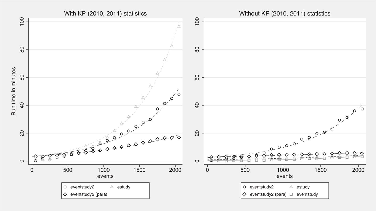
When one compares run times across community-contributed commands, it is important to recall some of their conceptual differences; see figure 1 for a visual comparison. eventstudy does not calculate any test statistics, which is why it is generally expected to be the fastest command in all scenarios. eventstudy2 calculates and reports all available test statistics during every run and provides extensive data management capabilities. estudy, on the other hand, provides only one test statistic per run but provides it for each event firm separately. Thus, the prediction of run time for eventstudy2 compared with estudy is less clear.

Figure 1.

Execution times of event studies with 50 to 2,050 events

The left graph in figure 1 plots the run times for eventstudy2, eventstudy2 with the parallel option, and estudy against the numbers of events. estudy is run with the diagnosticsstat(KP) option and eventstudy2‘s option nokolari is not enabled, which in both instances triggers the calculation of the most calculation-intense Kolari and Pynnönen (KP) (2010, 2011) statistics. The graphs point toward an exponential growth of run time with a considerably higher growth rate for estudy. While eventstudy2 can execute event studies with 2,000 events in less than an hour, the run time for estudy approaches 100 minutes.⁴ Further, the graph clearly demonstrates the benefits of the parallel option of eventstudy2, which already breaks even at around 700 events and is associated with a much lower growth rate. An event study with 2,000 events can be calculated in less than 20 minutes.

The right graph in figure 1 shows the run time when estudy is run with the diagnosticsstat(Norm) option and eventstudy2 with the nokolari option, which suppress the calculation of the KP (2010, 2011) statistics. It also shows the run time of eventstudy, which does not provide any test statistics. The growth rate for estudy drops substantially, which demonstrates that much of the priorly observed sensitivity of the run time to the number of events is attributable to computing the KP (2010) statistic. However, eventstudy2‘s run time depends less on test statistics, which are fully implemented in Mata, but is largely driven by its comprehensive data management routines (for example, implementing the Maynes and Rumsey [1993] algorithm for handling thinly traded stocks) and reporting routines (reporting which events had to be dropped and for which reason).

As I demonstrated in my analysis of published event studies in section 3, most event studies comprise more than only a few thousand events. Therefore, I record the run time in hours of the three community-contributed commands for studies with samples of 5,000, 10,000, 30,000, 60,000, 90,000, and 120,000 events, if feasible, in table 4. I measure run times with and without the calculation of the KP (2010, 2011) statistics (as in figure 1).

Table 4.

Run time in hours of community-contributed event-study commands

	eventstudy
Events	No test statistics available
5,000	0.3
10,000	1.0
>11,000	eventstudy hits the matsize limit of 11,000.
	eventstudy2
Events	With KP (2010, 2011) statistics	Without KP (2010, 2011) statistics
5,000	4.7	3.6
10,000	19.6	14.9
15,000	43.1	31.5
30,000	169.5	129.2
>30,000	Feasible but strong exponential growth.
	eventstudy2, parallel
Events	With KP (2010, 2011) statistics	Without KP (2010, 2011) statistics
5,000	1.4	0.2
10,000	4.9	0.4
15,000	11.5	0.5
30,000	45.2	1.0
60,000	Feasible	but 2.5
90,000	strong exponential growth	4.4
120,000	…	6.6
>120,000	…	Feasible.
	estudy
Events	With KP (2010, 2011) statistics	Without KP (2010, 2011) statistics
5,000	26.6	0.4
10,000	250.9	2.1
15,000	>24 days	5.7
23,000	>50 days	20.2
>24,000	estudy hits the maximum variables limit of 120,000.

Most notably, my tests reveal that eventstudy hits Stata/MP 16’s matsize limit of 11,000 when asked to calculate an event study with 11,000 or more events. estudy hits the maximum number of variables limit of 120,000 when asked to calculate event studies with 24,000 or more events. Further, the run time of estudy increases drastically for larger samples when asked to calculate the KP (2010, 2011) statistics to spend 250.9 hours on a study with only 10,000 events will most likely be considered impracticable by most researchers. eventstudy2 can perform this task in 19.6 hours (4.9 hours in parallel computing mode) because it loads the abnormal return matrices fully into Mata and calculates cross-correlations there, which is much more computationally efficient than correlating Stata variables.⁵ Although estudy theoretically can run larger event studies with the KP (2010, 2011) statistics, I cannot obtain results for the 15,000 events sample after 24 days of uninterrupted calculation. However, an analysis of the time that estudy requires to calculate the cross-correlation of one event’s abnormal returns with all other events’ abnormal returns during the estimation windows allows me to estimate a lower boundary for the 23,000 events sample, which is at least 50 days of run time.

Without being asked to calculate KP (2010, 2011) statistics, estudy is considerably faster than eventstudy2. However, eventstudy2 retakes the lead if run in parallel computing mode on 40 cores.

To conclude on the issue of run time, eventstudy and estudy are not suitable to run bigger event studies because of their handling of Stata/MP 16’s limits. If the user is interested in obtaining KP (2010, 2011) statistics, the practical limits of estudy kick in much earlier than the theoretically feasible 23,000 events.

4.2 Consistency of results and thin trading

While calculation times, as demonstrated in the previous subsection, differ substantially across the three community-contributed event-study commands, the abnormal returns and test statistics they calculate should be consistent. To test this presumption, I use the previously described setting with 100 randomly selected event samples and repeat the analysis 100 times, each time using each of the 3 commands on the selected sample. I calculate CAARs for days [0], [1], [0; 1], and [−1; 1] as well as the KP (2010) statistics when using eventstudy2 and estudy. Untabulated results show that all metrics exhibit almost perfect correlation across commands, which implies consistency in this ideal setting where no return data are missing.

However, in real-world settings, researchers commonly have to handle stock return data when stocks trade infrequently (thin trading). Let us assume the following scenario: a stock has a continuously compounded abnormal return of −2% on the event day [0] and +2% on the day after the event day [+1]. On the event day, however, the stock is not traded, which means that its abnormal return is not observable. The day after the event day, when the stock resumes trading, the observable abnormal return will be 0 because the closing price on this day will match the closing price on the day before the event day [−1]. How should an event-study command handle such situations? Ideally, it recognizes that the return observed on day [+1] is a cumulated return and excludes it from the calculation of the abnormal return on day [+1]. Nevertheless, it should include this return observation in the calculation of the CAARs, CAAR[0, 1]. Further, the missing return on day [0] should not be set to 0 but excluded from the calculation of the average abnormal event day return, AAR[0]. eventstudy2 follows these rules by implementing the Maynes and Rumsey (1993) algorithm for the handling of trade-to-trade returns and thinly traded stocks. The help files of eventstudy and estudy do not explain how the commands deal with this issue.

To get a better understanding of the ability of three community-contributed commands to handle thin trading, I artificially and randomly define half the event day [0] returns as thinly traded, which means that the return is compounded into the following day [+1] before being set to missing. Before introducing thin trading, I add a random return to the return on day [0] and subtract the same return on day [+1]. Thus, we know the true AAR[0] and AAR[+1] as well as that the CAAR[0, +1] and CAAR[−1, +1] are truly 0. Again, I perform 100 runs of 100 randomly selected samples using each of the three community-contributed event-study commands.

The upper left graph in figure 2 shows plots of measured average abnormal event day [0] returns on artificially induced abnormal returns. All three commands provide estimates that are close to the ideal 45 ^◦ -line through the origin and are thus unbiased. Thus, none of the three commands erroneously attributes a zero return to the missing return observations that result from thin trading or nontrading. However, the results differ with respect to day [+1] (upper right graph), where estudy and eventstudy systemically underestimate the return reversal because they attribute some of the abnormal event day returns to day [+1]. Only eventstudy2 realizes that about half the day [+1] returns are confounded with day [0], at that time unobservable, returns.

Figure 2.

CAAR calculation with thin trading on the event day

The lower left graph in figure 2 demonstrates that this error is mitigated in the calculating of CAAR[0, 1] by eventstudy by first calculating CARs by event firm and across time and then averaging them across event firms (the latter has to be performed by the user). estudy, however, appears to first calculate AARs by time and across events and then averages them across time, which entertains the bias and creates an overestimation in terms of the absolute value of CAAR[0, 1], which in my simulation is 0 by construction. In my simulation of perfect abnormal return reversal within one trading day, the bias is linearly related to the fraction of thinly traded stocks (50% in my simulation) and the induced abnormal return. For instance, we see that if half of event day returns suffer from thin trading and the induced abnormal return is 5%, estudy overestimates CAAR[0, +1] by about 2.5 percentage points. As can be seen from the graph in the lower right, the bias does not get weaker if the window is extended to three days, that is, CAAR[−1, +1].

To conclude, all three commands provide consistent results if thin trading is not present. If, however, thin trading is an issue and the return data are trade-to-trade returns, only eventstudy2 provides unbiased results.

5 Conclusion

All three commands discussed in this article, eventstudy, eventstudy2, and estudy, are useful in conducting event studies as they are commonly performed in the accounting, finance, and management literature. In terms of completeness as I define it—that is, availability of test statistics and benchmark models, handling of thin trading and reporting on dropped observations—my command eventstudy2 surpasses its alternatives. However, the other commands have superior input (eventstudy) or output (estudy) routines, which might make them the better choice for users who are operating with smaller samples or do not require complex test statistics. The estudy command might be particularly suited for analyses of data that come from Datastream as opposed to WRDS, because data that are extracted with Datastream request tables that typically come in wide rather than long format. The user should ensure, though, that his or her sample firms do not suffer from thin trading and that the sample is sufficiently small. Overall, given the three available community-contributed commands, there is no need for Stata users to leave their preferred programming environment to conduct event studies.

Finally, because I am often asked about that via email or most recently at the 2020 Stata Conference, I would like to briefly explain the differences between the three community-contributed commands and the Stata code that is offered at the Princeton University website.⁶ The Princeton code is a very useful starting point for writing one’s own event-study code because it provides a good overview on how to initially organize the data. However, it does not provide any advanced hypothesis testing or input–output routines. Developing an event-study command takes years of intense work. estudy.ado has more than 1,400 and eventstudy2.ado more than 1,700 lines of code, and although the amount of code does not necessarily predict the quality of command, it can provide a hint to its complexity and thus functionality. If at all, the roughly 40 lines of code on the Princeton website are comparable, in terms of functionality, with the eventstudy but not the other two commands.

Footnotes

Acknowledgments

I thank Joe Newton (the editor) and an anonymous referee for their valuable contributions. I also thank the attendees of the 2020 Stata Conference and all users whose feedback has substantially improved this article and the eventstudy2 command.

Notes

A Appendix

Below are tables of event studies in three leading field journals published during the period 2009–2018.

References

Abarbanell

Park

2017. Do bright-line earnings surprises really affect stock price reactions? Management Science 63: 1063–1084. https://doi.org/10.1287/mnsc.2015.2376.

Abrahamson

Jenkinson

Jones

2011. Why don’t U.S. issuers demand European fees for IPOs? Journal of Finance 66: 2055–2082. https://doi.org/10.1111/j.1540-6261.2011.01699.x.

Agarwal

Chen

V. Y. S.

Zhang

2016. The information value of credit rating action reports: A textual analysis. Management Science 62: 2218–2240. https://doi.org/10.1287/mnsc.2015.2243.

Agarwal

Jiang

Tang

Yang

2013. Uncovering hedge fund skill from the portfolio holdings they hide. Journal of Finance 68: 739–783. https://doi.org/10.1111/jofi.12012.

Aggarwal

Saffi

P. A. C.

Sturgess

2015. The role of institutional investors in voting: Evidence from the securities lending market. Journal of Finance 70: 2309–2346. https://doi.org/10.1111/jofi.12284.

Agrawal

Kamakura

W. A.

1995. The economic worth of celebrity endorsers: An event study analysis. Journal of Marketing 59: 56–62. https://doi.org/10.2307/1252119.

Ahern

K. R.

Harford

2014. The importance of industry links in merger waves. Journal of Finance 69: 527–576. https://doi.org/10.1111/jofi.12122.

Akbas

. 2016. The calm before the storm. Journal of Finance 71: 225–266. https://doi.org/10.1111/jofi.12377.

Albuquerque

Schroth

2015. The value of control and the costs of illiquidity. Journal of Finance 70: 1405–1455. https://doi.org/10.1111/jofi.12207.

10.

Allee

K. D.

DeAngelis

M. D.

2015. The structure of voluntary disclosure narratives: Evidence from tone dispersion. Journal of Accounting Research 53: 241–274. https://doi.org/10.1111/1475-679X.12072.

11.

Ammann

Horsch

Oesch

2016. Competing with superstars. Management Science 62: 2842–2858. https://doi.org/10.1287/mnsc.2015.2266.

12.

Anderson

R. C.

Reeb

D. M.

Zhao

2012. Family-controlled firms and informed trading: Evidence from short sales. Journal of Finance 67: 351–385. https://doi.org/10.1111/j.1540-6261.2011.01714.x.

13.

Anderson

R. W.

Bustamante

M. C.

Guibaud

Zervos

2018. Agency, firm growth, and managerial turnover. Journal of Finance 73: 419–464. https://doi.org/10.1111/jofi.12583.

14.

Arikan

A. M.

Stulz

R. M.

2016. Corporate acquisitions, diversification, and the firm’s life cycle. Journal of Finance 71: 139–194. https://doi.org/10.1111/jofi.12362.

15.

Ashbaugh-Skaife

Collins

D. W.

Kinney

W. R.

Jr. LaFond

2009. The effect of SOX internal control deficiencies on firm risk and cost of equity. Journal of Accounting Research 47: 1–43. https://doi.org/10.1111/j.1475-679X.2008.00315.x.

16.

Asquith

Mullins

D. W.

1983. The impact of initiating dividend payments on shareholders’ wealth. Journal of Business 56: 77–96. https://doi.org/10.1086/296187.

17.

Babenko

2009. Share repurchases and pay-performance sensitivity of employee compensation contracts. Journal of Finance 64: 117–150. https://doi.org/10.1111/j.1540-6261.2008.01430.x.

18.

Badoer

D. C.

James

C. M.

2016. The determinants of long-term corporate debt issuances. Journal of Finance 71: 457–492. https://doi.org/10.1111/jofi.12264.

19.

Ball

Brown

1968. An empirical evaluation of accounting income numbers. Journal of Accounting Research 6: 159–178. https://doi.org/10.2307/2490232.

20.

Barber

B. M.

Lyon

J. D.

1997. Detecting long-run abnormal stock returns: The empirical power and specification of test statistics. Journal of Financial Economics 43: 341–372. https://doi.org/10.1016/S0304-405X(96)00890-2.

21.

Becher

D. A.

Cohn

J. B.

Juergens

J. L.

2015. Do stock analysts influence merger completion? An examination of postmerger announcement recommendations . Management Science 61: 2430–2448. https://doi.org/10.1287/mnsc.2014.2065.

22.

Berkman

Koch

P. D.

Westerholm

P. J.

2014. Informed trading through the accounts of children. Journal of Finance 69: 363–404. https://doi.org/10.1111/jofi.12043.

23.

Berkman

Truong

2009. Event day 0? After-hours earnings announcements. Journal of Accounting Research 47: 71–103. https://doi.org/10.1111/j.1475-679X.2008.00312.x.

24.

Bernhardt

Wan

Xiao

2016. The reluctant analyst. Journal of Accounting Research 54: 987–1040. https://doi.org/10.1111/1475-679X.12120.

25.

Betton

Eckbo

B. E.

Thompson

Thorburn

K. S.

2014. Merger negotiations with stock market feedback. Journal of Finance 69: 1705–1745. https://doi.org/10.1111/jofi.12151.

26.

Bhagat

Romano

2002a. Event studies and the law: Part I: Technique and corporate litigation. American Law and Economics Review 4: 141–168. https://doi.org/10.1093/aler/4.1.141.

27.

Bhagat

Romano

2002b. Event studies and the law: Part II: Empirical studies of corporate law. American Law and Economics Review 4: 380–423. https://doi.org/10.1093/aler/4.2.380.

28.

Bhojraj

Hribar

Picconi

McInnis

2009. Making sense of cents: An examination of firms that marginally miss or beat analyst forecasts. Journal of Finance 64: 2361–2388. https://doi.org/10.1111/j.1540-6261.2009.01503.x.

29.

Blankespoor

Hendricks

B. E.

Miller

G. S.

2017. Perceptions and price: Evidence from CEO presentations at IPO roadshows. Journal of Accounting Research 55: 275–327. https://doi.org/10.1111/1475-679X.12164.

30.

Boehmer

Musumeci

Poulsen

A. B.

1991. Event-study methodology under conditions of event-induced variance. Journal of Financial Economics 30: 253–272. https://doi.org/10.1016/0304-405X(91)90032-F.

31.

Bowen

R. M.

Castanias

R. P.

Daley

L. A.

1983. Intra-industry effects of the accident at Three Mile Island. Journal of Financial and Quantitative Analysis 18: 87–111. https://doi.org/10.2307/2330806.

32.

Bradley

Gokkaya

Liu

2017. Before an analyst becomes an analyst: Does industry experience matter? Journal of Finance 72: 751–792. https://doi.org/10.1111/jofi.12466.

33.

Brennan

M. J.

Huh

S.-W.

Subrahmanyam

2016. Asymmetric effects of informed trading on the cost of equity capital. Management Science 62: 2460–2480. https://doi.org/10.1287/mnsc.2015.2250.

34.

Brown

S. J.

Warner

J. B.

1980. Measuring security price performance. Journal of Financial Economics 8: 205–258. http://dx.doi.org/10.1016/0304-405X(80)90002-1.

35.

Brown

S. J.

Warner

J. B.

1985. Using daily stock returns: The case of event studies. Journal of Financial Economics 14: 3–31. https://doi.org/10.1016/0304-405X(85)90042-X.

36.

Brown

S. V.

Tucker

J. W.

2011. Large-sample evidence on firms’ year-over-year MD&A modifications. Journal of Accounting Research 49: 309–346. https://doi.org/10.1111/j.1475-679X.2010.00396.x.

37.

Bruno

Cornaggia

K. J.

2016. Does regulatory certification affect the information content of credit ratings? Management Science 62: 1578–1597. https://doi.org/10.1287/mnsc.2015.2188.

38.

Bushee

B. J.

Core

J. E.

Guay

Hamm

S. J.

2010. The role of the business press as an information intermediary. Journal of Accounting Research 48: 1–19. https://doi.org/10.1111/j.1475-679X.2009.00357.x.

39.

Bushee

B. J.

Jung

M. J.

Miller

G. S.

2011. Conference presentations and the disclosure milieu. Journal of Accounting Research 49: 1163–1192. https://doi.org/10.1111/j.1475-679X.2011.00426.x.

40.

Bushman

R. M.

Williams

C. D.

Wittenberg-Moerman

2017. The informational role of the media in private lending. Journal of Accounting Research 55: 115–152. https://doi.org/10.1111/1475-679X.12131.

41.

Call

A. C.

Martin

G. S.

Sharp

N. Y.

Wilde

J. H.

2018. Whistleblowers and outcomes of financial misrepresentation enforcement actions. Journal of Accounting Research 56: 123–171. https://doi.org/10.1111/1475-679X.12177.

42.

Cao

S. S.

Narayanamoorthy

G. S.

2012. Earnings volatility, post–earnings announcement drift, and trading frictions. Journal of Accounting Research 50: 41–74. https://doi.org/10.1111/j.1475-679X.2011.00425.x.

43.

Cao

Dhaliwal

Yang

Y. G.

2015. Are all independent directors equally informed? Evidence based on their trading returns and social networks . Management Science 61: 795–813. https://doi.org/10.1287/mnsc.2013.1892.

44.

Capron

Pistre

2002. When do acquirers earn abnormal returns? Strategic Management Journal 23: 781–794. https://doi.org/10.1002/smj.262.

45.

Cen

Dasgupta

Sen

2016. Discipline or disruption? Stakeholder relationships and the effect of takeover threat . Management Science 62: 2820–2841. https://doi.org/10.1287/mnsc.2015.2252.

46.

Chang

Y. Y.

Dasgupta

Hilary

2010. CEO ability, pay, and firm performance. Management Science 56: 1633–1652. https://doi.org/10.1287/mnsc.1100.1205.

47.

Chava

Huang

Johnson

S. A.

2018. The dynamics of borrower reputation following financial misreporting. Management Science 64: 4775–4797. https://doi.org/10.1287/mnsc.2017.2739.

48.

Cheong

F. S.

Thomas

2018. Management of reported and forecast EPS, investor responses, and research implications. Management Science 64: 4277–4301. https://doi.org/10.1287/mnsc.2017.2832.

49.

Chhaochharia

Grinstein

Grullon

Michaely

2017. Product market competition and internal governance: Evidence from the Sarbanes—Oxley Act. Management Science 63: 1405–1424. https://doi.org/10.1287/mnsc.2015.2409.

50.

Choudhary

Rajgopal

Venkatachalam

2009. Accelerated vesting of employee stock options in anticipation of FAS 123-R. Journal of Accounting Research 47: 105–146. https://doi.org/10.1111/j.1475-679X.2008.00316.x.

51.

Christensen

H. B.

Lee

Walker

2009. Do IFRS reconciliations convey information? The effect of debt contracting. Journal of Accounting Research 47: 1167–1199. https://doi.org/10.1111/j.1475-679X.2009.00345.x.

52.

Cohen

Schmidt

2009. Attracting flows by attracting big clients. Journal of Finance 64: 2125–2151. https://doi.org/10.1111/j.1540-6261.2009.01496.x.

53.

Cohn

J. B.

Gillan

S. L.

Hartzell

J. C.

2016. On enhancing shareholder control: A (Dodd-) frank assessment of proxy access. Journal of Finance 71: 1623–1668. https://doi.org/10.1111/jofi.12402.

54.

Collin-Dufresne

Fos

2015. Do prices reveal the presence of informed trading? Journal of Finance 70: 1555–1582. https://doi.org/10.1111/jofi.12260.

55.

Collins

D. W.

Kothari

S. P.

1989. An analysis of the intertemporal and crosssectional determinants of earnings response coefficients. Journal of Accounting and Economics 11: 143–181. http://dx.doi.org/10.1016/0165-4101(89)90004-9.

56.

Corrado

1989. A nonparametric test for abnormal security-price performance in event studies. Journal of Financial Economics 23: 385–395. https://doi.org/10.1016/0304-405X(89)90064-0.

57.

Corrado

C. J.

2011. Event studies: A methodology review. Accounting & Finance 51: 207–234. https://doi.org/10.1111/j.1467-629X.2010.00375.x.

58.

Corrado

C. J.

Zivney

T. L.

1992. The specification and power of the sign test in event study hypothesis tests using daily stock returns. Journal of Financial and Quantitative Analysis 27: 465–478. https://doi.org/10.2307/2331331.

59.

Cowan

A. R.

1992. Nonparametric event study tests. Review of Quantitative Finance and Accounting 2: 343–358. https://doi.org/10.1007/BF00939016.

60.

Crane

A. D.

Koch

2018. Shareholder litigation and ownership structure: Evidence from a natural experiment. Management Science 64: 5–23. https://doi.org/10.1287/mnsc.2016.2561.

61.

Crawford

Gray

Johnson

B. R.

Price

R. A.

2018. What motivates buy-side analysts to share recommendations online? Management Science 64: 2574–2589. https://doi.org/10.1287/mnsc.2017.2749.

62.

Cready

Kumas

Subasi

2014. Are trade size-based inferences about traders reliable? Evidence from institutional earnings-related trading. Journal of Accounting Research 52: 877–909. https://doi.org/10.1111/1475-679X.12056.

63.

Cready

W. M.

Gurun

U. G.

2010. Aggregate market reaction to earnings announcements. Journal of Accounting Research 48: 289–334. https://doi.org/10.1111/j.1475-679X.2010.00368.x.

64.

Cuñat

Gine

Guadalupe

2012. The vote is cast: The effect of corporate governance on shareholder value. Journal of Finance 67: 1943–1977. https://doi.org/10.1111/j.1540-6261.2012.01776.x.

65.

Engelberg

Gao

2011. In search of attention. Journal of Finance 66: 1461–1499. https://doi.org/10.1111/j.1540-6261.2011.01679.x.

66.

Daniel

Grinblatt

Titman

Wermers

1997. Measuring mutual fund performance with characteristic-based benchmarks. Journal of Finance 52: 1035–1058. https://doi.org/10.1111/j.1540-6261.1997.tb02724.x.

67.

de Bodt

Cousin

J.-G.

Roll

2018. Full-stock-payment marginalization in merger and acquisition transactions. Management Science 64: 760–783. https://doi.org/10.1287/mnsc.2016.2635.

68.

De Franco

Vasvari

F. P.

Wittenberg-Moerman

2009. The informational role of bond analysts. Journal of Accounting Research 47: 1201–1248. https://doi.org/10.1111/j.1475-679X.2009.00348.x.

69.

DeHaan

Madsen

Piotroski

J. D.

2017. Do weather-induced moods affect the processing of earnings news? Journal of Accounting Research 55: 509–550. https://doi.org/10.1111/1475-679X.12160.

70.

Dellavigna

Pollet

J. M.

2009. Investor inattention and Friday earnings announcements. Journal of Finance 64: 709–749. https://doi.org/10.1111/j.1540-6261.2009.01447.x.

71.

Demerjian

Lev

McVay

2012. Quantifying managerial ability: A new measure and validity tests. Management Science 58: 1229–1248. https://doi.org/10.1287/mnsc.1110.1487.

72.

Dimitrov

Jain

P. C.

2011. It’s showtime: Do managers report better news before annual shareholder meetings? Journal of Accounting Research 49: 1193–1221. https://doi.org/10.1111/j.1475-679X.2011.00419.x.

73.

Doidge

Dyck

2015. Taxes and corporate policies: Evidence from a quasi natural experiment. Journal of Finance 70: 45–89. https://doi.org/10.1111/jofi.12101.

74.

Doidge

Karolyi

G. A.

Stulz

R. M.

2010. Why do foreign firms leave U.S. equity markets? Journal of Finance 65: 1507–1553. https://doi.org/10.1111/j.1540-6261.2010.01577.x.

75.

Donelson

D. C.

Hopkins

J. J.

2016. Large market declines and securities litigation: Implications for disclosing adverse earnings news. Management Science 62: 3183–3198. https://doi.org/10.1287/mnsc.2015.2306.

76.

Døskeland

T. M.

Hvide

H. K.

2011. Do individual investors have asymmetric information based on work experience? Journal of Finance 66: 1011–1041. https://doi.org/10.1111/j.1540-6261.2011.01658.x.

77.

Doyle

J. T.

Magilke

M. J.

2013. Decision usefulness and accelerated filing deadlines. Journal of Accounting Research 51: 549–581.

78.

Drake

M. S.

Roulstone

D. T.

Thornock

J. R.

2012. Investor information demand: Evidence from Google searches around earnings announcements. Journal of Accounting Research 50: 1001–1040. https://doi.org/10.1111/j.1475-679X.2012.00443.x.

79.

Durnev

Mangen

2009. Corporate investments: Learning from restatements. Journal of Accounting Research 47: 679–720. https://doi.org/10.1111/j.1475-679X.2009.00332.x.

80.

Dyck

Morse

Zingales

2010. Who blows the whistle on corporate fraud? Journal of Finance 65: 2213–2253. https://doi.org/10.1111/j.1540-6261.2010.01614.x.

81.

Dyreng

S. D.

Hoopes

J. L.

Wilde

J. H.

2016. Public pressure and corporate tax behavior. Journal of Accounting Research 54: 147–186. https://doi.org/10.1111/1475-679X.12101.

82.

Edmans

Goldstein

Jiang

2012. The real effects of financial markets: The impact of prices on takeovers. Journal of Finance 67: 933–971. https://doi.org/10.1111/j.1540-6261.2012.01738.x.

83.

Engelberg

Sasseville

Williams

2012. Market madness? The case of mad money. Management Science 58: 351–364. https://doi.org/10.1287/mnsc.1100.1290.

84.

Ertimur

Ferri

Oesch

2013. Shareholder votes and proxy advisors: Evidence from say on pay. Journal of Accounting Research 51: 951–996. https://doi.org/10.1111/1475-679X.12024.

85.

Falato

Milbourn

2015. Which skills matter in the market for CEOs? Evidence from pay for CEO credentials. Management Science 61: 2845–2869. https://doi.org/10.1287/mnsc.2014.2024.

86.

Fama

E. F.

Fisher

Jensen

M. C.

Roll

1969. The adjustment of stock prices to new information. International Economic Review 10: 1–21.

87.

Fama

E. F.

French

K. R.

1993. Common risk factors in the returns on stocks and bonds. Journal of Financial Economics 33: 3–56. https://doi.org/10.1016/0304-405X(93)90023-5.

88.

Fama

E. F

French

K. R.

2015. A five-factor asset pricing model. Journal of Financial Economics 116: 1–22. https://doi.org/10.1016/j.jfineco.2014.10.010.

89.

Fang

V. W.

Huang

A. H.

Karpoff

J. M.

2016. Short selling and earnings management: A controlled experiment. Journal of Finance 71: 1251–1294. https://doi.org/10.1111/jofi.12369.

90.

Fang

V. W.

Huang

A. H.

Wang

2017. Imperfect accounting and reporting bias. Journal of Accounting Research 55: 919–962. https://doi.org/10.1111/1475-679X.12170.

91.

Fernando

C. S.

May

A. D.

Megginson

W. L.

2012. The value of investment banking relationships: Evidence from the collapse of Lehman Brothers. Journal of Finance 235–270. https://doi.org/10.1111/j.1540-6261.2011.01711.x.

92.

Firth

Lin

Liu

Xuan

2013. The client is king: Do mutual fund relationships bias analyst recommendations? Journal of Accounting Research 51: 165–200. https://doi.org/10.1111/j.1475-679X.2012.00469.x.

93.

Flammer

2015. Does corporate social responsibility lead to superior financial performance? A regression discontinuity approach. Management Science 61: 2549–2568. https://doi.org/10.1287/mnsc.2014.2038.

94.

Fosfuri

Giarratana

M. S.

2009. Masters of war: Rivals’ product innovation and new advertising in mature product markets. Management Science 55: 181–191. https://doi.org/10.1287/mnsc.1080.0939.

95.

Fracassi

Tate

2012. External networking and internal firm governance. Journal of Finance 67: 153–194. https://doi.org/10.1111/j.1540-6261.2011.01706.x.

96.

Franco

Ittner

C. D.

Urcan

2017. Determinants and trading performance of equity deferrals by corporate outside directors. Management Science 63: 114–138. https://doi.org/10.1287/mnsc.2015.2332.

97.

Huang

2016. The persistence of long-run abnormal returns following stock repurchases and offerings. Management Science 62: 964–984. https://doi.org/10.1287/mnsc.2015.2150.

98.

Fung

S. Y. K.

Gul

F. A.

Radhakrishnan

2014. Investment banks’ entry into new IPO markets and IPO underpricing. Management Science 60: 1297–1316. https://doi.org/10.1287/mnsc.2013.1817.

99.

Gande

Saunders

2012. Are banks still special when there is a secondary market for loans? Journal of Finance 67(5): 1649–1684. https://doi.org/10.1111/j.1540-6261.2012.01769.x.

100.

Garfinkel

J. A.

2009. Measuring investors’ opinion divergence. Journal of Accounting Research 47: 1317–1348. https://doi.org/10.1111/j.1475-679X.2009.00344.x.

101.

Giannetti

Liao

2015. The brain gain of corporate boards: Evidence from China. Journal of Finance 70: 1629–1682. https://doi.org/10.1111/jofi.12198.

102.

Gilje

E. P.

Taillard

J. P.

2016. Do private firms invest differently than public firms? Taking cues from the natural gas industry. Journal of Finance 71: 1733–1778. https://doi.org/10.1111/jofi.12417.

103.

Gillan

S. L.

Hartzell

J. C.

Parrino

2009. Explicit versus implicit contracts: Evidence from CEO employment agreements. Journal of Finance 64: 1629–1655. https://doi.org/10.1111/j.1540-6261.2009.01475.x.

104.

Goldman

E. M.

Huang

P. P.

2015. Contractual vs. actual separation pay following CEO turnover. Management Science 61: 1108–1120. https://doi.org/10.1287/mnsc.2014.1988.

105.

Golubov

Petmezas

Travlos

N. G.

2012. When it pays to pay your investment banker: New evidence on the role of financial advisors in M&As. Journal of Finance 67: 271–311. https://doi.org/10.1111/j.1540-6261.2011.01712.x.

106.

Gorton

Kahl

Rosen

R. J.

2009. Eat or be eaten: A theory of mergers and firm size. Journal of Finance 64: 1291–1344. https://doi.org/10.1111/j.1540-6261.2009.01465.x.

107.

Green

T. C.

Hwang

B.-H.

2012. Initial public offerings as lotteries: Skewness preference and first-day returns. Management Science 58: 432–444. https://doi.org/10.1287/mnsc.1110.1431.

108.

Gurun

U. G.

Johnston

Markov

2016. Sell-side debt analysts and debt market efficiency. Management Science 62: 682–703. https://doi.org/10.1287/mnsc.2014.2145.

109.

Hail

Tahoun

Wang

2014. Dividend payouts and information shocks. Journal of Accounting Research 52: 403–456. https://doi.org/10.1111/1475-679X.12040.

110.

Halpern

1983. Corporate acquisitions: A theory of special cases? A review of event studies applied to acquisitions . Journal of Finance 38: 297–317. https://doi.org/10.2307/2327962.

111.

Hartzmark

S. M.

Shue

2018. A tough act to follow: Contrast effects in financial markets. Journal of Finance 73(4): 1567–1613. https://doi.org/10.1111/jofi.12685.

112.

Hendershott

Madhavan

2015. Click or call? Auction versus search in the over-the-counter market . Journal of Finance 70: 419–447. https://doi.org/10.1111/jofi.12164.

113.

Henry

T. R.

Koski

J. L.

2017. Ex-dividend profitability and institutional trading skill. Journal of Finance 72: 461–494. https://doi.org/10.1111/jofi.12472.

114.

Hilary

Hsu

Wang

2014. Management forecast consistency. Journal of Accounting Research 52: 163–191. https://doi.org/10.1111/1475-679X.12033.

115.

Hill

Schneeweis

1983. The effect of Three Mile Island on electric utility stock prices: A note. Journal of Finance 38: 1285–1292. https://doi.org/10.1111/j.1540-6261.1983.tb02297.x.

116.

Hirshleifer

Lim

S. S.

Teoh

S. H.

2009. Driven to distraction: Extraneous events and underreaction to earnings news. Journal of Finance 64: 2289–2325. https://doi.org/10.1111/j.1540-6261.2009.01501.x.

117.

Hobson

J. L.

Mayew

W. J.

Venkatachalam

2012. Analyzing speech to detect financial misreporting. Journal of Accounting Research 50: 349–392. https://doi.org/10.1111/j.1475-679X.2011.00433.x.

118.

Hsu

H.-C.

Reed

A. V.

Rocholl

2010. The new game in town: Competitive effects of IPOs. Journal of Finance 65: 495–528. https://doi.org/10.1111/j.1540-6261.2009.01542.x.

119.

Huang

A. H.

Lehavy

Zang

A. Y.

Zheng

2018. Analyst information discovery and interpretation roles: A topic modeling approach. Management Science 64: 2833–2855. https://doi.org/10.1287/mnsc.2017.2751.

120.

Huang

Hilary

2018. Zombie board: Board tenure and firm performance. Journal of Accounting Research 56: 1285–1329. https://doi.org/10.1111/1475-679X.12209.

121.

Hui

K. W.

Yeung

P. E.

2013. Underreaction to industry-wide earnings and the post-forecast revision drift. Journal of Accounting Research 51: 701–737. https://doi.org/10.1111/1475-679X.12006.

122.

Hutton

Jiang

Kumar

2015. Political values, culture, and corporate litigation. Management Science 61: 2905–2925. https://doi.org/10.1287/mnsc.2014.2106.

123.

Ibbotson

R. G.

1975. Price performance of common stock new issues. Journal of Financial Economics 2: 235–272. https://doi.org/10.1016/0304-405X(75)90015-X.

124.

Iliev

2010. The effect of SOX Section 404: Costs, earnings quality, and stock prices. Journal of Finance 65: 1163–1196. https://doi.org/10.1111/j.1540-6261.2010.01564.x.

125.

Jagolinzer

A. D.

2009. SEC Rule 10b5-1 and insiders’ strategic trade. Management Science 55: 224–239. https://doi.org/10.1287/mnsc.1080.0928.

126.

Jagolinzer

A. D.

Larcker

D. F.

Taylor

D. J.

2011. Corporate governance and the information content of insider trades. Journal of Accounting Research 49: 1249–1274. https://doi.org/10.1111/j.1475-679X.2011.00424.x.

127.

Jame

Johnston

Markov

Wolfe

M. C.

2016. The value of crowdsourced earnings forecasts. Journal of Accounting Research 54: 1077–1110. https://doi.org/10.1111/1475-679X.12121.

128.

Jenter

Lewellen

2015. CEO preferences and acquisitions. Journal of Finance 70: 2813–2852. https://doi.org/10.1111/jofi.12283.

129.

Jenter

Lewellen

Warner

J. B.

2011. Security issue timing: What do managers know, and when do they know it? Journal of Finance 66: 413–443. https://doi.org/10.1111/j.1540-6261.2010.01638.x.

130.

Jiang

Wang

2012. Hedge funds and Chapter 11. Journal of Finance 67: 513–560. https://doi.org/10.1111/j.1540-6261.2012.01724.x.

131.

Jiang

Mei

2018. Influencing control: Jawboning in risk arbitrage. Journal of Finance 73: 2635–2675. https://doi.org/10.1111/jofi.12721.

132.

Jin

Livnat

Zhang

2012. Option prices leading equity prices: Do option traders have an information advantage? Journal of Accounting Research 50: 401–432. https://doi.org/10.1111/j.1475-679X.2012.00439.x.

133.

Johnson

T. L.

E. C.

2018. Asymmetric trading costs prior to earnings announcements: Implications for price discovery and returns. Journal of Accounting Research 56: 217–263. https://doi.org/10.1111/1475-679X.12189.

134.

Jorion

Zhang

2009. Credit contagion from counterparty risk. Journal of Finance 64: 2053–2087. https://doi.org/10.1111/j.1540-6261.2009.01494.x.

135.

Kadyrzhanova

Rhodes-Kropf

2011. Concentrating on governance. Journal of Finance 66: 1649–1685. https://doi.org/10.1111/j.1540-6261.2011.01684.x.

136.

Kahl

Shivdasani

Wang

2015. Short-term debt as bridge financing: Evidence from the commercial paper market. Journal of Finance 70: 211–255. https://doi.org/10.1111/jofi.12216.

137.

Kalaignanam

Kushwaha

Steenkamp

J.-B. E. M.

Tuli

K. R.

2013. The effect of CRM outsourcing on shareholder value: A contingency perspective. Management Science 59: 748–769. https://doi.org/10.1287/mnsc.1120.1565.

138.

Kane

Lee

Y. K.

Marcus

1984. Earnings and dividend announcements: Is there a corroboration effect? Journal of Finance 39: 1091–1099. https://doi.org/10.1111/j.1540-6261.1984.tb03894.x.

139.

Kaniel

Liu

Saar

Titman

2012. Individual investor trading and return patterns around earnings announcements. Journal of Finance 67: 639–680. https://doi.org/10.1111/j.1540-6261.2012.01727.x.

140.

Karolyi

G. A.

Taboada

A. G.

2015. Regulatory arbitrage and cross-border bank acquisitions. Journal of Finance 70: 2395–2450. https://doi.org/10.1111/jofi.12262.

141.

Karolyi

S. A.

2018. Personal lending relationships. Journal of Finance 73: 5–49. https://doi.org/10.1111/jofi.12589.

142.

Karpoff

J. M.

Lou

2010. Short sellers and financial misconduct. Journal of Finance 65: 1879–1913. https://doi.org/10.1111/j.1540-6261.2010.01597.x.

143.

Kaspereit

2015. eventstudy2: Stata module to perform event studies with complex test statistics. Statistical Software Components S458086, Department of Economics, Boston College. https://ideas.repec.org/c/boc/bocode/s458086.html.

144.

Kecskés

Michaely

Womack

K. L.

2017. Do earnings estimates add value to sell-side analysts’ investment recommendations? Management Science 63: 1855–1871. https://doi.org/10.1287/mnsc.2015.2385.

145.

Keung

Lin

Z.-X.

Shih

2010. Does the stock market see a zero or small positive earnings surprise as a red flag? Journal of Accounting Research 48: 105–136. https://doi.org/10.1111/j.1475-679X.2009.00354.x.

146.

Kim

Song

2015. Management earnings forecasts and value of analyst forecast revisions. Management Science 61: 1663–1683. https://doi.org/10.1287/mnsc.2014.1920.

147.

Klein

Zur

2009. Entrepreneurial shareholder activism: Hedge funds and other private investors. Journal of Finance 64: 187–229. https://doi.org/10.1111/j.1540-6261.2008.01432.x.

148.

Knittel

C. R.

Stango

2014. Celebrity endorsements, firm value, and reputation risk: Evidence from the Tiger Woods scandal. Management Science 60: 21–37. https://doi.org/10.1287/mnsc.2013.1749.

149.

Koester

Lundholm

Soliman

2016. Attracting attention in a limited attention world: Exploring the causes and consequences of extreme positive earnings surprises. Management Science 62: 2871–2896. https://doi.org/10.1287/mnsc.2015.2286.

150.

Kolari

J. W.

Pynnönen

2010. Event study testing with cross-sectional correlation of abnormal returns. Review of Financial Studies 23: 3996–4025. https://doi.org/10.1093/rfs/hhq072.

151.

Kolari

J. W

Pynnönen

2011. Nonparametric rank tests for event studies. Journal of Empirical Finance 18: 953–971. https://doi.org/10.1016/j.jempfin.2011.08.003.

152.

Kolasinski

A. C.

Reed

A. V.

Ringgenberg

M. C.

2013. A multiple lender approach to understanding supply and search in the equity lending market. Journal of Finance 68: 559–595. https://doi.org/10.1111/jofi.12007.

153.

Kothari

Warner

2007. The econometrics of event studies. In Handbook of Corporate Finance: Empirical Corporate Finance, ed. B. E. Eckbo. Vol. 1, chap. 1, 3–36. Amsterdam: Elsevier.

154.

Kothari

S. P.

Shu

Wysocki

P. D.

2009. Do managers withhold bad news? Journal of Accounting Research 47: 241–276. https://doi.org/10.1111/j.1475-679X.2008.00318.x.

155.

Krüger

Landier

Thesmar

2015. The WACC fallacy: The real effects of using a unique discount rate. Journal of Finance 70: 1253–1285. https://doi.org/10.1111/jofi.12250.

156.

Kumar

2010. Self-selection and the forecasting abilities of female equity analysts. Journal of Accounting Research 48: 393–435. https://doi.org/10.1111/j.1475-679X.2009.00362.x.

157.

Kutsuna

Smith

J. K.

Smith

R. L.

2009. Public information, IPO price formation, and long-run returns: Japanese evidence. Journal of Finance 64: 505–546. https://doi.org/10.1111/j.1540-6261.2008.01440.x.

158.

Lamb

R. P.

1998. An examination of market efficiency around hurricanes. Financial Review 33: 163–172. https://doi.org/10.1111/j.1540-6288.1998.tb01614.x.

159.

Lee

L. F.

Hutton

A. P.

Shu

2015. The role of social media in the capital market: Evidence from consumer product recalls. Journal of Accounting Research 53: 367–404. https://doi.org/10.1111/1475-679X.12074.

160.

Lee

L. F.

A. K.

2016. Do opinions on financial misstatement firms affect analysts’ reputation with investors? Evidence from reputational spillovers. Journal of Accounting Research 54(4): 1111–1148. https://doi.org/10.1111/1475-679X.12119.

161.

Lemmon

Liu

L. X.

Mao

M. Q.

Nini

2014. Securitization and capital structure in nonfinancial firms: An empirical investigation. Journal of Finance 69: 1787–1825. https://dx.doi.org/10.2139/ssrn.1964647.

162.

Leung

Veenman

2018. Non-GAAP earnings disclosure in loss firms. Journal of Accounting Research 56: 1083–1137. https://doi.org/10.1111/1475-679X.12216.

163.

Levi

Zhang

2010. Deal or no deal: Hormones and the mergers and acquisitions game. Management Science 56(9): 1462–1483. https://doi.org/10.1287/mnsc.1100.1206.

164.

Levi

Zhang

X.-J.

2015. Do temporary increases in information asymmetry affect the cost of equity? Management Science 61: 354–371. https://doi.org/10.1287/mnsc.2013.1887.

165.

Zhang

2015. Short selling pressure, stock price behavior, and management forecast precision: Evidence from a natural experiment. Journal of Accounting Research 53: 79–117. https://doi.org/10.1111/1475-679X.12068.

166.

Loh

R. K.

Stulz

R. M.

2018. Is sell-side research more valuable in bad times? Journal of Finance 73: 959–1013. https://doi.org/10.1111/jofi.12611.

167.

Loughran

Mcdonald

2011. When is a liability not a liability? Textual analysis, dictionaries, and 10-Ks. Journal of Finance 66: 35–65. https://doi.org/10.1111/j.1540-6261.2010.01625.x.

168.

Loughran

Mcdonald

2014. Measuring readability in financial disclosures. Journal of Finance 69: 1643–1671. https://doi.org/10.1111/jofi.12162.

169.

Louis

Sun

2010. Investor inattention and the market reaction to merger announcements. Management Science 56: 1781–1793. https://doi.org/10.1287/mnsc.1100.1212.

170.

Louis

Sun

A. X.

Urcan

2013. Do analysts sacrifice forecast accuracy for informativeness? Management Science 59: 1688–1708. https://doi.org/10.1287/mnsc.1120.1675.

171.

Loureiro

Taboada

A. G.

2015. Do improvements in the information environment enhance insiders’ ability to learn from outsiders? Journal of Accounting Research 53: 863–905. https://doi.org/10.1111/1475-679X.12082.

172.

Lui

Markov

Tamayo

2012. Equity analysts and the market’s assessment of risk. Journal of Accounting Research 50: 1287–1317. https://doi.org/10.1111/j.1475-679X.2012.00462.x.

173.

Lyon

J. D.

Barber

B. M.

Tsai

C.-L.

1999. Improved methods for tests of long-run abnormal stock returns. Journal of Finance 54: 165–201. https://doi.org/10.1111/0022-1082.00101.

174.

MacKinlay

A. C.

1997. Event studies in economics and finance. Journal of Economic Literature 35: 13–39.

175.

Madsen

2017. Anticipated earnings announcements and the customer–supplier anomaly. Journal of Accounting Research 55: 709–741. https://doi.org/10.1111/1475-679X.12158.

176.

Manchiraju

Rajgopal

2017. Does corporate social responsibility (CSR) create shareholder value? Evidence from the Indian Companies Act 2013. Journal of Accounting Research 55: 1257–1300. https://doi.org/10.1111/1475-679X.12174.

177.

Manconi

Massa

Zhang

2018. The informational role of corporate hedging. Management Science 64: 3843–3867. https://doi.org/10.1287/mnsc.2016.2717.

178.

Martin

Shalev

2017. Target firm-specific information and acquisition efficiency. Management Science 63: 672–690. https://doi.org/10.1287/mnsc.2015.2371.

179.

Masulis

R. W.

Mobbs

2011. Are all inside directors the same? Evidence from the external directorship market. Journal of Finance 66: 823–872. https://doi.org/10.1111/j.1540-6261.2011.01653.x.

180.

Masulis

R. W.

Wang

Xie

2009. Agency problems at dual-class companies. Journal of Finance 64: 1697–1727. https://doi.org/10.1111/j.1540-6261.2009.01477.x.

181.

Mayew

W. J.

Venkatachalam

2012. The power of voice: Managerial affective states and future firm performance. Journal of Finance 67: 1–43. https://doi.org/10.1111/j.1540-6261.2011.01705.x.

182.

Maynes

Rumsey

1993. Conducting event studies with thinly traded stocks. Journal of Banking & Finance 17: 145–157. https://doi.org/10.1016/0378-4266(93)90085-R.

183.

McNally

W. J.

Shkilko

Smith

B. F.

2017. Do brokers of insiders tip other clients? Management Science 63: 317–332. https://doi.org/10.1287/mnsc.2015.2287.

184.

Michels

2017. Disclosure versus recognition: Inferences from subsequent events. Journal of Accounting Research 55: 3–34. https://doi.org/10.1111/1475-679X.12128.

185.

Milian

J. A.

2015. Unsophisticated arbitrageurs and market efficiency: Overreacting to a history of underreaction? Journal of Accounting Research 53: 175–220. https://doi.org/10.1111/1475-679X.12070.

186.

Nguyen

B. D.

Nielsen

K. M.

2014. What death can tell: Are executives paid for their contributions to firm value? Management Science 60: 2994–3010. https://doi.org/10.1287/mnsc.2014.2011.

187.

Oxley

J. E.

Sampson

R. C.

Silverman

B. S.

2009. Arms race or détente? How interfirm alliance announcements change the stock market valuation of rivals. Management Science 55: 1321–1337. https://doi.org/10.1287/mnsc.1090.1022.

188.

Pacicco

Vena

Venegoni

2018. Event study estimations using Stata: The estudy command. Stata Journal 18: 461–476. https://doi.org/10.1177/1536867X1801800211.

189.

Pacicco

Vena

Venegoni

2019. estudy: Stata module to perform an event study. Statistical Software Components S458628, Department of Economics, Boston College. https://ideas.repec.org/c/boc/bocode/s458628.html.

190.

Pacicco

Vena

Venegoni

2021. From common to firm-specific event dates: A new version of the estudy command. Stata Journal 21: 141–151. https://doi.org/10.1177/1536867X211000010.

191.

Patell

J. M.

1976. Corporate forecasts of earnings per share and stock price behavior: Empirical test. Journal of Accounting Research 14: 246–276. https://doi.org/10.2307/2490543.

192.

Peress

2010. Product market competition, insider trading, and stock market efficiency. Journal of Finance 65: 1–43. https://doi.org/10.1111/j.1540-6261.2009.01522.x.

193.

Qian

Zhu

J. L.

2018. Return to invested capital and the performance of mergers and acquisitions. Management Science 64: 4818–4834. https://doi.org/10.1287/mnsc.2017.2766.

194.

Rajamani

van der Poel

de Jong

Ongena

2017. The international diversification of banks and the value of their cross-border M&A advice. Management Science 63: 2211–2232. https://doi.org/10.1287/mnsc.2015.2396.

195.

Ransbotham

Mitra

2010. Target age and the acquisition of innovation in high-technology industries. Management Science 56: 2076–2093. https://doi.org/10.1287/mnsc.1100.1223.

196.

Robinson

A. B.

Tuli

K. R.

Kohli

A. K.

2015. Does brand licensing increase a licensor’s shareholder value? Management Science 61: 1436–1455. https://doi.org/10.1287/mnsc.2014.1980.

197.

Ryngaert

Thomas

2012. Not all related party transactions (RPTs) are the same: Ex ante versus ex post RPTs. Journal of Accounting Research 50: 845–882. https://doi.org/10.1111/j.1475-679X.2012.00437.x.

198.

Savor

Wilson

2016. Earnings announcements and systematic risk. Journal of Finance 71: 83–138. https://doi.org/10.1111/jofi.12361.

199.

Savor

P. G.

2009. Do stock mergers create value for acquirers? Journal of Finance 64: 1061–1097. https://doi.org/10.1111/j.1540-6261.2009.01459.x.

200.

Serfling

. 2016. Firing costs and capital structure decisions. Journal of Finance 71: 2239–2286. https://doi.org/10.1111/jofi.12403.

201.

Servaes

Tamayo

2014. How do industry peers respond to control threats? Management Science 60: 380–399. https://doi.org/10.1287/mnsc.2013.1773.

202.

Seybert

Yang

H. I.

2012. The party’s over: The role of earnings guidance in resolving sentiment-driven overvaluation. Management Science 58: 308–319. https://doi.org/10.1287/mnsc.1110.1386.

203.

Sheen

2014. The real product market impact of mergers. Journal of Finance 69: 2651–2688. https://doi.org/10.1111/jofi.12200.

204.

Shenoy

2012. An examination of the efficiency, foreclosure, and collusion rationales for vertical takeovers. Management Science 58: 1482–1501. https://doi.org/10.1287/mnsc.1110.1498.

205.

Shon

Veliotis

2013. Insiders’ sales under rule 10b5-1 plans and meeting or beating earnings expectations. Management Science 59: 1988–2002. https://doi.org/10.1287/mnsc.1120.1669.

206.

Shroff

Sun

A. X.

White

H. D.

Zhang

2013. Voluntary disclosure and information asymmetry: Evidence from the 2005 securities offering reform. Journal of Accounting Research 51: 1299–1345. https://doi.org/10.1111/1475-679X.12022.

207.

Silvers

2016. The valuation impact of SEC enforcement actions on nontarget foreign firms. Journal of Accounting Research 54: 187–234. https://doi.org/10.1111/1475-679X.12098.

208.

Solomon

D. H.

2012. Selective publicity and stock prices. Journal of Finance 67: 599–638. https://doi.org/10.1111/j.1540-6261.2012.01726.x.

209.

Spiegel

Tookes

2013. Dynamic competition, valuation, and merger activity. Journal of Finance 68: 125–172. https://doi.org/10.1111/j.1540-6261.2012.01796.x.

210.

Teoh

S. H.

Wong

T. J.

1993. Perceived auditor quality and the earnings response coefficient. Accounting Review 68: 346–366.

211.

Thirumalai

Sinha

K. K.

2011. Product recalls in the medical device industry: An empirical exploration of the sources and financial consequences. Management Science 57: 376–392. https://doi.org/10.1287/mnsc.1100.1267.

212.

von Lilienfeld-Toal

Ruenzi

2014. CEO ownership, stock market performance, and managerial discretion. Journal of Finance 69: 1013–1050. https://doi.org/10.1111/jofi.12139.

213.

Vyas

2011. The timeliness of accounting write-downs by U.S. financial institutions during the financial crisis of 2007–2008. Journal of Accounting Research 49: 823–860. https://doi.org/10.1111/j.1475-679X.2011.00410.x.

214.

Wang

2014. Accounting standards harmonization and financial statement comparability: Evidence from transnational information transfer. Journal of Accounting Research 52: 955–992. https://doi.org/10.1111/1475-679X.12055.

215.

Wang

Welker

2011. Timing equity issuance in response to information asymmetry arising from IFRS adoption in Australia and Europe. Journal of Accounting Research 49: 257–307. https://doi.org/10.1111/j.1475-679X.2010.00392.x.

216.

Wilcoxon

1945. Individual comparisons by ranking methods. Biometrics Bulletin 1: 80–83. https://doi.org/10.2307/3001968.

217.

Williams

2013. Financial analysts and the false consensus effect. Journal of Accounting Research 51: 855–907. https://doi.org/10.1111/1475-679X.12016.

218.

Zhang

2013. eventstudy: Stata module to perform event studies in finance. Statistical Software Components S457615, Department of Economics, Boston College. https://econpapers.repec.org/software/bocbocode/s457615.htm.

219.

Zhao

2017. Does information intensity matter for stock returns? Evidence from Form 8-K filings. Management Science 63: 1382–1404. https://doi.org/10.1287/mnsc.2015.2408.

Event studies with daily stock returns in Stata: Which command to use?

Abstract

Keywords

1 Introduction

2 Conceptual characteristics of event studies and community-contributed commands

2.1 Elements of event studies

2.2 Software requirements

2.3 Features of community-contributed commands

3 Applicability to event studies in leading field journals

4 Practical limitations

4.1 Run time

4.2 Consistency of results and thin trading

5 Conclusion

Footnotes

Acknowledgments

Notes

A Appendix

References