The estudy command proposed by Pacicco, Vena, and Venegoni (2018, Stata Journal 18: 461–476) performs event studies only for event-date clustering, that is, when the event date is common to all securities. This constitutes a relevant limitation because the vast majority of this methodology’s applications concerns studies in which the events happen on different dates for each statistical unit considered. In this article, we propose and describe a substantial update to estudy, which 1) performs event studies in the absence of event-date clustering (that is, when each security has its own event date); 2) further customizes the output by producing LATEX-formatted tables; 3) graphs the cumulative abnormal returns over a customized period set by the user; 4) makes more output data available through either the return list or Excel files; 5) allows a double possibility as input: either prices or returns; and 6) uses wildcards.
Pacicco, Vena, and Venegoni (2018) presented estudy, a community-contributed command to perform an event study. estudy allows the user to rely on a flexible framework that can be customized in several ways, from the definition of the estimation window or the event window or windows, to the choice of the statistical model necessary to estimate abnormal returns (ARs), to the parametric and nonparametric statistical tests for their significance.
This contribution remained limited in its applicability because it was suited only to studying events happening on the same date for all the firms in the sample. This is quite binding because the vast majority of event studies’ applications resides in the fields of corporate finance and accounting, where events take place on different dates for each firm. This article aims to fix this lacuna by presenting and describing a substantial update that extends the reach and scope of Pacicco, Vena, and Venegoni (2018) in several ways. More specifically, this version of estudy improves on the former because it now allows the user to
perform event studies for a sample of firms with different event dates, extending the more specific setup (that is, an event study with event-date clustering) proposed in the first release;
produce LATEX-formatted output tables;
graph the cumulative ARs over a customized period set by the user around the (firm-specific or common) event date;
retrieve more outputs through either the return list or the Excel file;
handle securities’ and indices’ prices as inputs; and
This article focuses on the new features and changes to Pacicco, Vena, and Venegoni (2018). With respect to omitted options, the reader may refer directly to both Pacicco, Vena, and Venegoni (2018) and the estudy help file. As with Pacicco, Vena, and Venegoni (2018), estudy still allows the specification of different securities in one to N varlists, separately analyzed. As thoroughly explained by MacKinlay (1997), Kothari and Warner (2007), and Corrado (2011), among others, an event study allows one to estimate the portion of return exclusively determined by the event taking place. It does so by disentangling the ex post actual returns of securities in two parts: the normal return, which is the portion unaffected by the event, and the AR, which measures the impact of the event on securities’ returns. In other words, the cumulative AR (CAR) represents the actual net return of securities compared with their normal, expected components. Because this portion of return is taken out from the actual ex post realization, the CAR represents the share of the return solely determined by the event. Using returns as inputs is no longer strictly required, because the user can now perform an event study starting from securities’ prices.
2.1 Options
As previously mentioned, in this section, we focus on the description of the options that were added or changed in the command presented by Pacicco, Vena, and Venegoni (2018).
evdate(string | namelist datelist) specifies the date or dates of the event. For common event dates (that is, event-date clustering), no matter the format of datevar(), evdate() must be expressed as mmddyyyy, ddmmyyyy, or yyyymmdd according to the dateformat() specified—MDY, DMY, or YMD, respectively. For different event dates, two variables must be specified: the first is namelist, with the names of the securities studied (exactly as reported in varlists), and the second is datelist, with the dates on which the event takes place for each security. evdate() is required.
outputfile(filename) specifies the name of the .xlsx file in which both the ARs (always without significance stars) and the p-values are stored in two separate sheets. The format imposed by suppress() is maintained. In the updated version, the test statistics and the standard errors of the CARs1 are stored in separate sheets. The command automatically replaces the file if it already exists.
price has to be specified when the input data are securities’ and indices’ prices instead of returns. The command then computes the returns and runs the event study as specified. When prices are used, the indices data (modtype(SIM), modtype(MFM), modtype(MAM) models) must be inputted as prices.
tex shows the output table in TEX format.
graph(# # [ , save ]) plots the graph ranging from the lower bound (that is, the first integer specified) to the upper bound (that is, the second integer specified). When the option save is specified, the graphs will not be shown but will be saved in the working directory. Otherwise, the graphs will be shown but not saved. This option is contingent on the suppress() option (when specified); if the individual ARs are suppressed, only group graphs will be created. Contrarily, if the portfolio ARs are suppressed, only individual graphs will be created.
detail shows the details of the estimation window length and the other features of the fitted model along with possible warnings that the community-contributed command issued.
3 What is new?
The changes made to estudy are the following:
The main innovation allows users to compute CARs when the event is not clustered on the same date for the securities that are considered. In this case, the user must specify two variables in the evdate(string | namelist datelist) option: namelist, with the names of the securities studied, and datelist, with the dates in which the event takes place for each security. This improvement allows the user to specify as many events as there are companies in N varlists. In this respect, notice here that the maximum number of companies that one can simultaneously analyze depends on the Stata version—from about 400 (Stata/IC) to more than 24,000 (for Stata/MP).
Specifying the tex option produces LATEX-formatted output tables in the Results window.
By specifying the graph(# # [ , save ]) option, one can graph the cumulative ARs over a user-customized period set around the (firm-specific or common) event date. The suboption save allows users to store them in the working directory, while, if it is not specified, the graph will be shown.
estudy produces more outputs through either the return list or the Excel file. Specifically, it now provides the estimated CARs, as well as their p-values and standard deviations (compare footnote 1); the values of the statistical tests adopted; and the time series of estimated ARs. Moreover, estudy stores the following in r():
The price option allows users to handle securities’ and indices’ prices as inputs.
The possibility to use wildcards. As varlists can be large, we allow users two shortcuts to write them. In particular, users can either put a - between two variables or use an *. The former includes all the variables between the two specified variables (as defined by the order they are listed in the Variables window); the latter includes all variables starting (or ending) with a given string.
4 Examples
We illustrate how estudy works using the dataset we provide called examples_estudy. This dataset contains the time series of returns and prices of 10 companies’ shares and the U.S. S&P 500 Index, as well as the returns of the three Fama and French (1993) factors. Also, the dataset includes two variables that are necessary to perform an event study with multiple event dates: security_names, which encompasses the varnames specified in all varlists,2 and event_dates, which specifies the firm-specific event date corresponding to each security specified in security_names. Through the following examples, we show how to use the updated version of the command and clarify how each option can be used to customize it, with a specific focus on the new or changed components, or both. As previously pointed out, the main change is the possibility to perform an event study without event-date clustering (that is, with multiple, firm-specific event dates); the command Pacicco, Vena, and Venegoni (2018) originally proposed performs event studies on common (single) event dates. Accordingly, this section first shows how to set the command to maintain its original scope (the event study in the case of event-date clustering), and the rest of the discussion is dedicated to an in-depth explanation of the novelties.
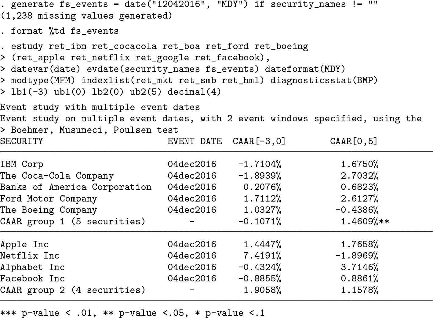
Thus, we start with a simple setup by performing an event study on two (separate) varlists with three event windows around the event date December 4, 2016. Because we are conducting an event study considering event-date clustering, the evdate() option specifies only one argument as string: the common event date. This latter item, coherently with the previous version of the command, must be specified in line with the dateformat() option (in this case, MDY, because the event date has the format mmd-dyyyy). The remaining options, unchanged in this update, specify a multifactor model (modtype()), the three Fama and French (1993) factors (indexlist()), the diagnostic to be implemented (diagnosticsstat()), and the number of decimals (decimal()) to be shown in the output tables.
As with the original version of the command, when the estimation window is not set, the command considers it, by default, to be from the first available observation to the 30th trading day prior to the event (−30 considering the event date as t = 0). A warning message reminds the user of the automatic setup of the estimation window when the option detail is specified. With respect to the output, the table header briefly recaps the setup of the event study performed, recounting the common event date, the number of event windows specified, and the diagnostic test implemented. The first column reports the labels of the variables under scrutiny, adding, by default, two rows per varlist to evaluate the impact of the event on the groups of securities. The first shows the CAR obtained through the portfolio approach, and the second shows the cumulative average abnormal return (CAAR). The remaining columns show CARs and CAARs over the event windows specified, identifying those that are statistically significant with asterisks, as explained by the legend at the bottom of the table. Horizontal lines separate the table into panels, with each showing the specified varlists. The results yielded by this application tell us that, in the specified event windows, the event that occurred on December 4, 2016, has not exercised a significant impact on all the firms included in the analysis with the sole exception of Ford, which reports a positive and significant AR over the [−3, 3] window. Moreover, the average CAAR of the first group over the [0, 5] event window reports a positive and significant AR, showing that the event might have exerted an effect at the aggregate level in the first group. From this, we can infer that some kind of news concerning this company and the group as a whole may have been released on that day. As previously mentioned, the changes implemented to estudy make the original command a particular case in this current version. In the next example, we show this by performing an event study on a common event date, which in this case corresponds to December 4, 2016, for all companies under scrutiny. We do so by specifying two arguments in the evdate() option: security_names, a string variable including at least the varnames specified in all varlists, and fs_events, a date variable that includes the same date (December 4, 2016) for all securities.
Because we are estimating the impact of a common event using the syntax for firm-specific event dates, the layout changes slightly (the last event window has been removed for the sake of exposition). Indeed, the second column shows the event date referred to for each company, while the portfolio return is no longer computed. Apart from these marginal differences, the reader can easily observe that the results yielded by this framework correspond to those in the previous example.
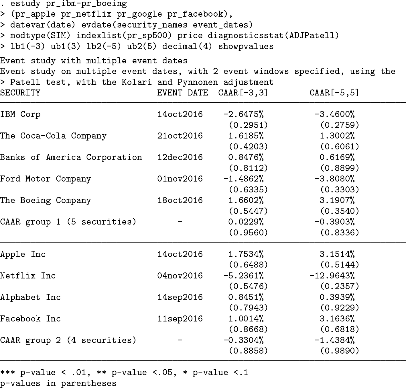
In the next example, we depart from event-date clustering and investigate companies affected by an event that takes place on different dates for each of them (for example, a dividend announcement, a CEO replacement). We do so by specifying two arguments in the evdate() option: the string variable security_names and event_dates, which is a date variable including the event date corresponding to each security under scrutiny. In addition, rather than specifying each single security, this time we specify more variables thanks to the wildcard - (first varlist). In line with the command that was originally submitted, the p-values are shown in parentheses below each CAAR because the show-pvalues option has been set.
Because we are now dealing with firm-specific events, the table header does not show any information regarding the event date but still recalls the implemented statistical test as well as the number of event windows.
Thanks to the wildcard -, the first varlist includes all variables stored in the dataset from ret_ibm to ret_boeing. Even though, in this specific case, the wildcard does not allow the user to save much space, its relevance becomes evident. Indeed, using the wildcard offers a twofold benefit: on the one hand, the user can save characters by typing a shorter command, and on the other hand, the user can avoid forgetting variables when the event study is conducted on a large set of securities.
Turning to the results, we see the events have not abnormally affected the returns of companies under scrutiny either individually or as a group. In economic terms, the events considered did not provide additional information to market participants.
The same results can be obtained by using securities’ prices instead of returns because the price option permits the user to directly handle them, as the next example clarifies.
We can easily observe that the results are unchanged; the only difference between the previous example and this one lies in the input data: the former relies on returns, while the latter relies on security prices (as emerges from the option price).
A new option made available with this release allows users to further customize the output format. Along these lines, the tex option permits users to obtain LATEX-formatted tables, which can be readily integrated into the TEX files. Below, we provide a concrete example by performing an event study with two varlists and two event windows over four trading days ([−3, 0]) and six trading days ([0, 5]).
Still, the events do not seem to provide new information, because none of the CARs and CAARs reach statistical significance.
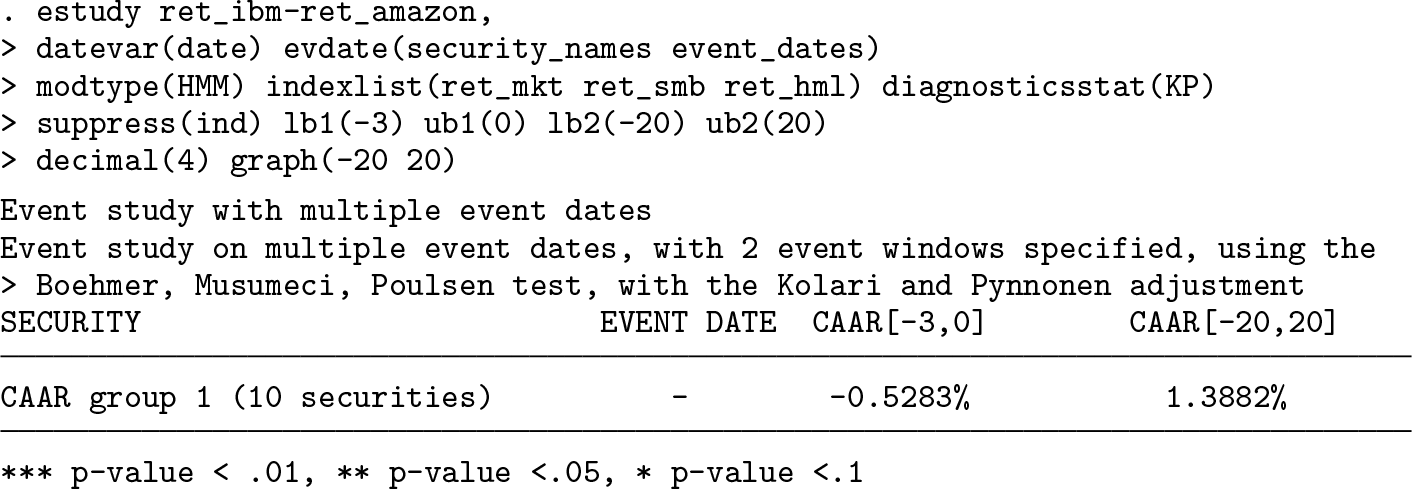
The last example is dedicated to the explanation of the graph() option. We thus show how to obtain the graphs of estimated CARs and CAARs over the customized range specified through the option (−20, +20). In other words, in the tth period, the graph shows the value of CAARs from the lower bound specified in the graph() option to period t. Accordingly, when the length of the event window is equal to the one in the graph, the last point of the graph corresponds to the value of the CAARs reported in the output table (the last column in this case).
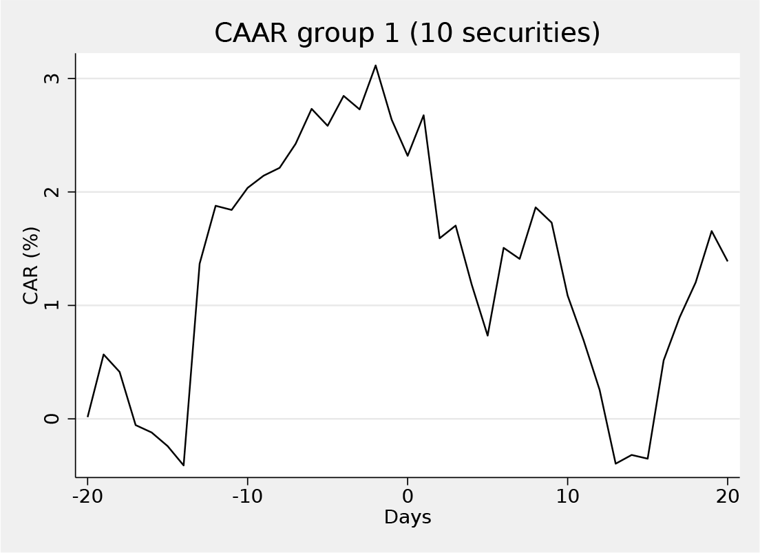
Because the suppress(ind) option has been set, estudy shows the corresponding graph on a group basis only.
The graph shows the CAAR in the specified period, which ranges from 20 days prior to the event to 20 days after the event
If the user specifies the suboption save of the graph() option, estudy does not show any graphs but rather stores them in the directory in use.
Supplemental Material
Supplemental Material, sj-zip-1-stj-10.1177_1536867X211000010 - From common to firm-specific event dates: A new version of the estudy command
Supplemental Material, sj-zip-1-stj-10.1177_1536867X211000010 for From common to firm-specific event dates: A new version of the estudy command by Fausto Pacicco, Luigi Vena and Andrea Venegoni in The Stata Journal
Footnotes
5 Programs and supplemental materials
To install a snapshot of the corresponding software files as they existed at the time of publication of this article, type
Please find the following supplemental material available below.
For Open Access articles published under a Creative Commons License, all supplemental material carries the same license as the article it is associated with.
For non-Open Access articles published, all supplemental material carries a non-exclusive license, and permission requests for re-use of supplemental material or any part of supplemental material shall be sent directly to the copyright owner as specified in the copyright notice associated with the article.