Sage Journals: Discover world-class research

Abstract

This article is primarily a replication study of Engle and Patton (2001, Quantitative Finance 1: 237–245), but it also serves as a demonstration of the time-series features introduced into Stata over the past two decades. The dataset used in the original study is extended from the end date of the original sample on 22 August 2000 to 1 August 2017 to examine the robustness of the models.

Keywords

st0637 volatility GARCH time series reproducible research

1 Introduction

The aim of this project is to reproduce Engle and Patton (2001) “What good is a volatility model” 20 years after it was first published in Quantitative Finance. The data used in the original article (hereafter referred to as EP) consisting of the Dow Jones Industrial Average Index and the three-month U.S. Treasury Bill rate for the period 23 August 1988 to 22 August 2000 are available for download.¹ The sample is later extended to include data up to 1 August 2017. This classic article is a nice introduction to volatility modeling for students of financial econometrics and represents a good target for reproducible research. It is also a vehicle to demonstrate some of the time-series features introduced in Stata over these two decades.

In a seminal article that is regarded as the starting point of the discipline of financial econometrics, Engle (1982) introduced the concept of autoregressive conditional heteroskedasticity (ARCH) to model a time-varying variance using a simple linear model. A generalization of the model due to Bollerslev (1986) is known as generalized autoregressive conditional heteroskedasticity (GARCH). In its simplest form, the model is given by

\begin{array}{l} y_{t} = μ + u_{t} \\ u_{t} ~ N (0, h_{t}) \\ h_{t} = ω + α u_{t - 1}^{2} + β h_{t - 1} \end{array}

The fundamental property of the model in (1), known as the GARCH(1,1) model, is that the conditional variance h_t is time varying with an autoregressive component, h_t ₋ ₁, and a component driven by unexpected events proxied by the squared disturbance in the previous period, $u_{t - 1}^{2}$ . In this model, the parameter β, where 0 ≤ β < 1, determines how past shocks affect the conditional variance at time t. The initial impact of the previous shock on h_t is α. It is this basic model and a few variations to it that EP estimate in their article.

For illustrative purposes, we do not include additional terms in the mean equation for y_t other than the constant term, µ; additional variables can be easily included. Similarly, the assumption of only one lag on both the squared error term, u_t ², and the conditional variance, h_t ₋ ₁, is only for ease of exposition. Additional terms in u_t ² ₋ ₂ , u_t ² ₋ ₃ ,… could be added to the variance equation as well as additional autoregressive terms h_t ₋ ₂ , h_t ₋ ₃ ,…, leading to a GARCH(p, q) model.

The rest of this article is structured as follows. In section 2, we review the data used by EP and highlight the characteristics of financial returns that give rise to GARCH modeling. In sections 3 to 7, we reproduce and explore the results reported by EP in section 3 of their article. Finally, in section 8, we extend the EP dataset from 22 August 2000 to 1 August 2017. The original models stand up well to this extension of the sample period, despite now including episodes of severe turbulence in the stock market.

2 Summary of the data

The daily data are observed only on days when the Dow Jones Index trades. Simply using the dates provided to tsset the data will yield a time series with gaps. This means that referring to the lag of the trading date will always use yesterday’s date (which may be a missing value) instead of the date of the previous trading day. There are two fixes. The first quick fix is simply to use the observation numbers as the time variable. This device ensures no gaps in the series, but it is a stop-gap approach that does not allow reference to calendar dates in analyzing the data and presenting results. A far better way of dealing with the problem involves creating user-defined business dates.

Designated as %tb dates, a business-daily calendar omits all dates on which there is no trading. In the current data, the date variable is called datevec; it is a daily date variable with missing values for all nontrading days. It would also be possible to use data in which the nontrading dates do not appear as observations. The code to make a business calendar named buscal.stbcal is as follows. After creating the calendar, Stata recognizes the new format %tbbuscal, and the Stata variable bcaldatevec is used to tsset the data.

The percentage log returns on the Dow Jones Index (djrets) are computed as

r_{t} = 100 \times (\log p_{t} - \log p_{t - 1})

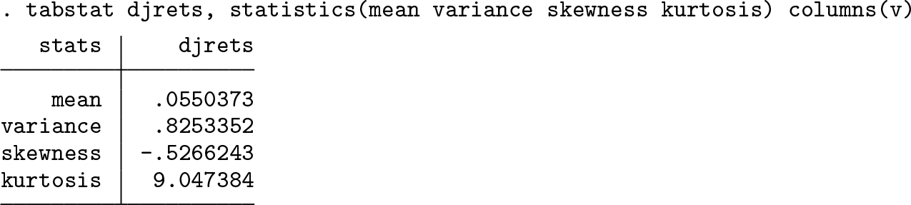
The summary statistics reported in EP table 1 are reproduced as follows:

Table 1.

Estimates of volatility models over varying horizons

Variable	Daily	2-day	3-day	4-day	Weekly
Constant	0.05955	0.11445	0.16660	0.21348	0.26258
ω	0.00717	0.01375	0.02312	0.02417	0.02072
α	0.03714	0.04193	0.05001	0.04260	0.04039
β	0.95458	0.94982	0.94155	0.95166	0.95733
EP HL	73	68	183	508	365
HL	84	168	246	482	1517

As this table shows, the index had a small positive average return of about one-twentieth of one percent per day. The daily variance was 0.8253, implying an average annualized volatility of 14.42%. The annualized volatility is computed as $\sqrt{252 σ^{2}}$ , where 252 is the median number of equity trading days per year in the United States and σ ² is the unconditional variance of the returns. The returns distribution is substantially negatively skewed, and the kurtosis coefficient indicates that the returns distribution has thicker tails than would be found in a Gaussian distribution, which has a kurtosis coefficient of 3. These “fat tails” are commonly found in high-frequency financial time series.

Figures 1 and 2 reproduce the daily index and returns, respectively. These figures illustrate many of the stylized facts about volatility alluded to in section 2 of EP.

Figure 1.

The Dow Jones Industrial Index, 23 August 1988 to 22 August 2000

Figure 2.

Returns on the Dow Jones Industrial Index, 23 August 1988 to 22 August 2000

1. From figure 1, it is apparent that the variance of the index changes over time as its growth is accompanied by ever-increasing swings.

2. Figure 2 displays volatility clustering in which periods of turbulence and periods of tranquility tend to cluster in time. The implication of such clustering is that volatility shocks today will influence the expectation of volatility many periods in the future.

3. Volatility is mean reverting. Mean reversion in volatility is generally interpreted as implying a normal level of volatility to which volatility will eventually return. Long-run forecasts of volatility should all converge to this same normal level of volatility, no matter when they are made. Thus, the volatility plot in figure 2 shows no trend.

4. Many proposed volatility models impose the assumption that the conditional volatility of the asset is affected symmetrically by positive and negative innovations. In the ARCH(1) and GARCH(1,1) models, for example, the variance is affected only by the square of the lagged innovation, disregarding the sign of that innovation. For equity returns, it is particularly unlikely that positive and negative shocks—“good news” and “bad news”—have the same impact on volatility. In figure 2, many negative returns are substantially larger than the largest positive returns. Assuming that these negative innovations are linked to bad news, it is reasonable to conjecture that bad news has a greater influence on volatility than does good news of a similar size.

Figure 3 presents the correlograms of the returns and the squared returns series, respectively. It is apparent from the correlogram of the returns that there is very little linear dependence in the series. This result is one of the important predictions of the celebrated efficient markets hypothesis (Fama 1970). Briefly, the efficient markets hypothesis states that current stock prices incorporate all relevant information so that all subsequent price changes represent random departures from previous prices. In an efficient market, therefore, the series of returns should show no time dependence. This result is in stark contrast to the correlogram of squared returns, where much stronger dependence is evident. This plot suggests that squared returns—and volatility—may be predictable.

Figure 3.

Correlograms of returns and squared returns

3 A volatility model

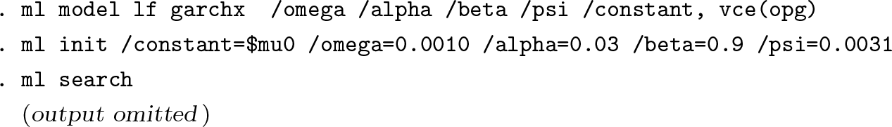
The parameters of the GARCH(1,1) model in (1) are estimated by maximum likelihood in Stata using the arch command. EP base their estimation of the assumption of normally distributed errors, as in (1), so that the log likelihood function for observation t is given by

l_{t} = - \frac{1}{2} \log 2 π - \frac{1}{2} \log h_{t} - \frac{1}{2} \frac{u_{t}^{2}}{h_{t}}

The starting value for the conditional variance h_t ₋ ₁ may be set in a few ways. The Stata default for arch is to use the unconditional variance, and this is the method chosen here. Given the values of the skewness and kurtosis coefficients reported previously, the assumption of Gaussian errors is not likely to be supported by the data. The estimates based on the normal log likelihood are therefore known as quasi–maximum likelihood estimates. It turns out that, in the GARCH model, the parameter estimates are still consistent but care must be taken when computing their standard errors. Most econometric packages now routinely support estimation of GARCH models based on different distributional assumptions. In Stata, the distribution() option of the arch command also supports the t distribution and the generalized error distribution, which allow estimation of the tail thickness of the error distribution.

There are two issues of note with these results. The first is that the coefficient estimates obtained here do not quite match those reported in table 2 of EP. The EP estimates of $\hat{α} = 0.0399$ and $\hat{β} = 0.9505$ are quite similar to those reported here, but this observation masks an important difference. In footnote 4 on page 242 of EP, the authors point out that a t test rejects the null hypothesis that $\hat{α} + \hat{β} \geq 1$ , known as integrated generalized autoregressive conditional heteroskedasticity (IGARCH). The confidence interval for the current estimates provided by the Stata nlcom command indicates that this is not the case for the estimates reported here.² EP does not report the value of the log-likelihood function at the optimum, thus making it difficult to ascertain which set of estimates are to be preferred. The value of the log-likelihood function obtained by Stata is −3920.313.

Table 2.

Estimates of the GARCH(1,1) models fit by EP using the extended data, 23 August 1988 to 1 August 2017. Robust standard errors are in parentheses.

	GARCH(1,1)	TARCH(1,1)	GARCH(1,1)-X
Constant	0.0548	0.0318	0.0549
	(0.0091)	(0.0087)	(0.0091)
ω^‡	0.0147	0.0180	−4.4891
	(0.0037)	(0.0042)	(0.2918)
α	0.0776	0.1302	0.0792
	(0.0106)	(0.0187)	(0.0108)
β	0.9077	0.9110	0.9049
	(0.0122)	(0.0125)	(0.0127)
φ		−0.1240
		(0.0188)
γ			0.0998
			(0.0546)
log likelihood	73	68	183

‡ The ω coefficient in the GARCH(1,1)-X model enters the conditional variance in exponentiated form.

The second issue of note relates to the standard errors. The standard errors reported in table 2 of EP are significantly smaller than those reported by Stata. This observation is important and masks an issue that is sometimes glossed over. The maximum likelihood estimates of the parameters of the GARCH model, based on the assumption of Gaussian errors, are consistent even if the true distribution of the innovations is not Gaussian. However, the usual standard errors of the estimators are not consistent when the assumption of Gaussian errors is violated. If the parameters of the model are collected into the vector θ , then standard errors can be estimated consistently using the so-called sandwich estimator,

VCE (θ) = T^{- 1} H^{- 1} (θ) J (θ) H^{- 1} (θ)

where H( θ ) is the second derivative of the log-likelihood function and J( θ ) is the outer product of the gradients matrix, respectively given by

H (θ) = \frac{1}{T} \sum_{t = 1}^{T} \frac{\partial^{2} l_{t}}{\partial θ \partial θ^{'}}, J (θ) = \frac{1}{T} \sum_{t = 1}^{T} \frac{\partial l_{t}}{\partial θ} \frac{\partial l_{t}}{\partial θ^{'}}

When using the vce(robust) option, Stata’s arch command reports standard errors based on implementing (3), a task that requires computing both the first and the second derivatives of the log-likelihood function. Bollerslev and Wooldridge (1992) provide a way of expressing H( θ ) in terms of first derivatives only. When implemented, the standard errors are known as Bollerslev–Wooldridge standard errors. From (2), the first and second derivatives of the log-likelihood function at time t are given by

\begin{array}{l} g_{t} = - \frac{1}{2} \frac{1}{h_{t}} \frac{\partial h_{t}}{\partial θ} (1 - \frac{u_{t}^{2}}{h_{t}}) \\ h_{t} = - \frac{1}{2} {- \frac{1}{h_{t}^{2}} \frac{\partial h_{t}}{\partial θ} \frac{\partial h_{t}}{\partial θ^{'}} (1 - \frac{u_{t}^{2}}{h_{t}}) + \frac{1}{h_{t}} \frac{\partial^{2} h_{t}}{\partial θ \partial θ^{'}} (1 - \frac{u_{t}^{2}}{h_{t}}) + \frac{1}{h_{t}^{2}} \frac{\partial h_{t}}{\partial θ} \frac{\partial h_{t}}{\partial θ^{'}} \frac{u_{t}^{2}}{h_{t}}} \end{array}

The conditional expectation of the first derivative taken at t − 1 is

E_{t - 1} (g_{t}) = - \frac{1}{2} \frac{1}{h_{t}} \frac{\partial h_{t}}{\partial θ} {1 - E_{t - 1} (\frac{u_{t}^{2}}{h_{t}})} = 0

because the variance of standardized residual $u_{t}^{2} / h_{t}$ is 1 in expectation. The second derivative now takes the simple form

E_{t - 1} (h_{t}) = E_{t - 1} (- \frac{1}{2} \frac{1}{h_{t}^{2}} \frac{\partial h_{t}}{\partial θ} \frac{\partial h_{t}}{\partial θ^{'}} \frac{u_{t}^{2}}{h_{t}})

requiring only the first derivatives. A consistent estimate of the matrix H( θ ) is

H (θ) = E {E_{t - 1} (h_{t})} = - \frac{1}{2} \frac{1}{T} \sum_{t = 1}^{T} \frac{1}{h_{t}^{2}} \frac{\partial h_{t}}{\partial θ} \frac{\partial h_{t}}{\partial θ^{'}} \frac{u_{t}^{2}}{h_{t}}

The discrepancy between the standard errors is then probably due to the difference between the Bollerslev–Wooldridge approach that uses first derivatives and the full sandwich estimator used by Stata.³

EP states that the choice of a GARCH(1,1) model is based on the Schwarz information criterion (SIC) after fitting GARCH(p, q) models and searching over p ∊ [1, 5] and q ∊ [1, 2]. The results of a similar search in Stata suggest that a GARCH(2,2) model gives the lowest SIC, which is then estimated.

The use of simple information criteria in the selection of GARCH models is known to be problematic (Brooks and Burke 2003). Without knowing exactly how EP computed the SIC, it is not possible to further explore the reasons for the discrepancy.⁴ Looking at the parameter estimates of the GARCH(2,2) model, however, it seems that although the specification gives a better SIC it does not look particularly sensible, in that the absolute values of the second-order terms are close in magnitude to the first-order terms. Here, therefore, as in most empirical applications, the GARCH(1,1) specification or some variant of a GARCH(1,1) model is a safe option. In this regard, it is also important to consider the work of Hansen and Lunde (2005), who find that the forecasts of conditional variance obtained from this simple model are always difficult to beat.

The final issue EP deal with in this subsection is whether or not the model has captured all of the persistence in the squared residuals. They suggest examining the correlogram of the standardized squared residuals. If the model’s specification is adequate, the standardized squared residuals should be serially uncorrelated.

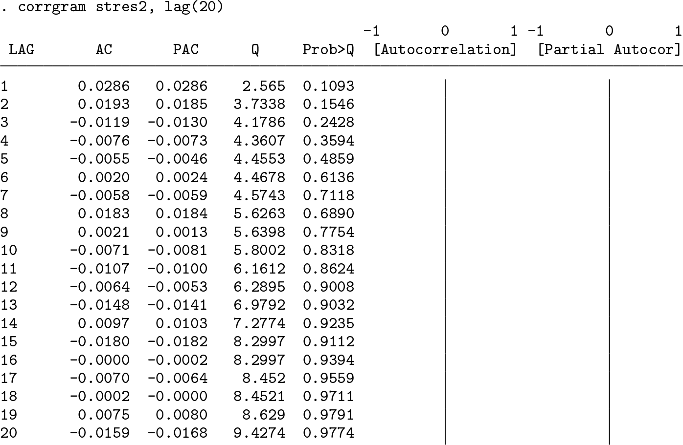
The Ljung–Box Q statistic at the twentieth lag of the standardized squared residuals is 9.4274, which is slightly different from the 8.9545 reported by EP. This slight difference is to be expected given that the parameter estimates and hence the standardized residuals differ slightly, but the overall conclusion holds: the standardized squared residuals are indeed serially uncorrelated.

4 Mean reversion and persistence in volatility

The results for the GARCH(1,1) model indicate that the volatility of returns is very persistent, with $\hat{α} + \hat{β} = 0.9917$ . EP find that the sum of these coefficients is 0.9904. One way of measuring the persistence of the process is in terms of the half-life (HL) of volatility, which is defined as the time taken for the volatility to move halfway back toward its unconditional mean following an impulse. Formally, HL is that smallest k for which

| h_{t + k | t} - {\bar{σ}}^{2} | = \frac{1}{2} | h_{t + 1 | t} - {\bar{σ}}^{2} |

where the long-run level to which volatility reverts is given by

{\bar{σ}}^{2} = \frac{ω}{1 - α - β}

A representation of the k-step-ahead mean-adjusted forecasting equation is given by (see, for example, Zivot [2009] for details)

h_{t + k | t} - {\bar{σ}}^{2} = {(α + β)}^{k - 1} (h_{t + 1 | t} - {\bar{σ}}^{2})

Substituting (6) into the definition of HL in (4) gives

{(α + β)}^{k - 1} | h_{t + 1 | t} - {\bar{σ}}^{2} | = \frac{1}{2} | h_{t + 1 | t} - {\bar{σ}}^{2} |

After simplifying and taking logs, a simple expression for the HL, k, is

k \approx \frac{\log (1 / 2)}{\log (α + β)}

The EP parameter estimates indicate an HL of 73 trading days, whereas the results reported here suggest an HL of about 84 trading days.

Notice that, from (6), it is apparent that as k → ∞, the volatility forecast tends to ${\bar{σ}}^{2}$ provided that α + β < 1. In other words, for the conditional variance to bestationary, the sum $\hat{α} + \hat{β}$ must be less than 1. If the sum is 1, then the process is known as an IGARCH process (Engle and Bollerslev 1986). Although EP find that the sum is significantly less than 1, the same is not true of the results reported here.

Although the unconditional variance of an IGARCH(1,1) process does not exist, Lumsdaine (1996) shows that standard asymptotically based inference procedures are generally valid even in the presence of IGARCH effects.⁵

The unconditional mean of the GARCH(1,1) process in (5) when calculated for the Dow Jones over the sample period turns out to be 0.8542, which implies that the mean annualized volatility over the sample was 14.77%.

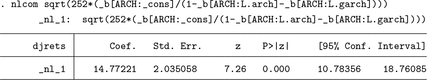
This estimate is slightly different from the 14.67% reported by EP, but this is to be expected given the slight discrepancies in parameter estimates. A plot of the annualized conditional volatility estimates over the sample period is given in figure 4. The conditional volatility is very similar to that plotted by EP. In fact, to the naked eye, the plots are identical notwithstanding the slight differences in parameter estimates.

Figure 4.

Estimated conditional volatility using a GARCH(1,1) model, August 1988– August 2000

The mean-reverting behavior of conditional volatility is evident in the patterns of dynamic forecasts of volatility. Following EP, dynamic forecasts of annualized daily volatility are produced starting at 23 August 1995 and 22 August 1997, respectively. The first of these forecasts was made at a date with unusually low volatility, and so the forecasts of volatility increase gradually to the unconditional level. The second forecast was made during a period of high volatility. The forecasts of volatility decrease slowly toward the unconditional level of volatility. Figure 5 demonstrates this pattern clearly.⁶

Figure 5.

Forecasts of daily return volatility using the GARCH(1,1) model

An alternative way of visualizing the mean reversion of volatility is in terms of figure 6 in EP. Our figure 6 below is based on Stata estimates of the GARCH(1,1) parameters and shows some differences with EP. In particular, the reversion to the mean in EP is not completed even within 200 days. In our figure, the adjustment is completed by about 150 days. The respective HL estimates based on the GARCH models are 73 days (EP) and 84 days (current estimate). Given the size of these half-lives, it seems more appropriate that the adjustment would be complete well before 200 days.

Figure 6.

Illustrating mean reversion in the forecasts of daily return volatility using the GARCH(1,1) model

EP suggest examining the volatility of volatility by observing the behavior of the k-period-ahead forecast volatility for different choices of k. In figure 7 below, which is similar to figure 7 of EP, forecasts are presented for horizons of one week (5 days), one quarter (62 days), and one year (252 days). It is expected that the movements in volatility forecasts will become more muted as the horizon increases. At one year ahead, the volatility forecasts should approach the estimated mean obtained from the GARCH(1,1) model of 14.77%. These forecasts are constructed using (6) with the appropriate index k.

Figure 7.

Forecast annualized volatilities for different horizons obtained from the GARCH(1,1) model. The solid horizontal line is the unconditional estimate of annualized volatility obtained from the fitted model of 14.77%.

Just as in the original EP article, it is immediately apparent that the movements at shorter horizons are larger than the movements at longer horizons. This pattern is an implication of the mean reversion in volatility.

5 An asymmetric volatility model

Based on the behavior of returns in figure 2, it was conjectured that the sign of the “news”, represented by the prior period’s residual, might influence the magnitude of the response in volatility. We can parameterize this concept in many ways, one of which is the threshold GARCH (or TARCH) model. This model was proposed by Glosten, Jagannathan, and Runkle (1993) and Zakoian (1994), motivated by the exponential GARCH model of Nelson (1991).

In Stata, the tarch() specification for the conditional variance is

h_{t} = ω + α u_{t - 1}^{2} + ϕ u_{t - 1}^{2} I (u_{t - 1} > 0) + β_{2} h_{t - 1}

where I(·) is the indicator function that takes the value 1 if (·) is true and 0 otherwise. This implies that the coefficients on the news will differ depending on whether news is good or bad:

effect of news on variance = {\begin{array}{l} α + ϕ & u_{t - 1} > 0 & good news \\ α & u_{t - 1} \leq 0 & bad news \end{array}

The presence of the leverage effect in Stata’s TARCH model requires that the coefficient φ is negative so that bad news has a greater impact on volatility than good news. Asymmetric effects will be present if the estimated φ is statistically distinguishable from 0. This specification is the opposite of that used by EP who define the indicator function as I(u_t ₋ ₁ > 0). To allow for non-Gaussian errors, we fit the model with a t distribution.

These results confirm the conclusion of EP that the sign of the news has a significant influence on the volatility of returns. The estimate of φ is negative and significant, with the effect on volatility summarized as follows:

effect of news on variance = {\begin{array}{l} 0.0637 - 0.0455 = 0.0182 & u_{t - 1} > 0 \\ 0.0637 & u_{t - 1} \leq 0 \end{array}

In other words, bad news at time t − 1 increases the volatility at time t by 3.5 times as much as good news of the same magnitude. This is a similar effect to that found by EP whose reported leverage effect is about four times greater for bad news. The estimated degrees of freedom of 5.3 strongly rejects Gaussian errors.

6 A model with exogenous volatility regressors

Exogenous regressors are dealt with in Stata by using the het( varlist ) option of the arch command. Stata adopts a slightly different approach from other econometric packages by specifying that the constant and the exogenous regressors enter the conditional variance equation in exponentiated form. For a single exogenous variable x_t , the conditional variance equation is

h_{t} = \exp (ω + γ x_{t}) + α u_{t - 1}^{2} + β h_{t - 1}

This specification allows the x_t variable to take on any values on the real line, while ensuring that the parenthesized expression is strictly positive.

EP used the lagged level of the three-month U.S. Treasury Bill rate as an exogenous regressor in their model of returns, arguing that the Treasury Bill rate is correlated with the cost of borrowing to firms and thus may carry information that is relevant to the volatility of returns. Estimation of the model yields the following results:

The impact of the lagged Treasury Bill rate is significant but not quite as significant as the EP results suggest. The downside of the estimation of the model in this exponentiated form is that it makes direct comparison with EP difficult. Using the ml command in Stata (see Gould, Pitblado, and Poi [2010] for details), the GARCH model in the form estimated by EP is easily programmed. Using the unconditional variance as the starting value for the conditional variance, the results obtained are as follows.

The positive sign on ψ, the lagged Treasury Bill coefficient, indicates that higher interest rates are generally associated with higher levels of volatility of equity returns. This result is taken to confirm those reported by Glosten, Jagannathan, and Runkle (1993), who also find that the Treasury Bill rate is positively related to equity return volatility. The problem, however, is that the coefficient estimate of ψ is insignificant. The problem seems to stem from the standard errors: the coefficients are similar to those reported by EP but the robust standard errors are much larger. Reestimating and using standard errors from the outer product of gradients matrix yields results very similar to EP.

It seems, therefore, that the standard errors reported in table 5 of EP are not robust.

On reflection, to counter the argument that Stata’s convention for dealing with exogenous variables is not as transparent as a simple linear form, there are at least two advantages to the exponentiated form of the het() model.

1. The contribution of the exogenous regressors is constrained to be positive. There is, therefore, no instance in which a particular combination of the value of the exogenous variable and its coefficient can cause a negative variance to occur.

2. Imposing this restriction has teased out a significant coefficient on the exogenous regressor when using robust standard errors, a result that is elusive if the nonexponentiated form is used.

7 Aggregation of volatility models

Volatility clustering and non-Gaussian behavior in financial returns is typically seen in weekly, daily, or intraday data. In the final subsection of their empirical example, EP provide evidence consistent with the theoretical result that the empirical results obtained are dependent on the sampling frequency. However, as shown in Drost and Nijman (1993), for GARCH models there is no simple aggregation principle that links the parameters of the model at one sampling frequency to the parameters at another frequency. This means that if a GARCH model is correctly specified for one frequency of data, then it will be misspecified for data with different time scales.

EP fit the simple GARCH(1,1) model on the data, sampled at different frequencies, and compute the HL for each of the models. The results are presented in table 1. While the results indicate that the sampling frequency affects the results in terms of coefficient estimates and HL, they also show that the original estimates presented in EP are quite different from those presented here.

Clearly, these are substantial differences, and while their statistical significance has not been assessed, there is some question as to why the original EP HL estimates are not monotonically increasing; in theory, the persistence of conditional volatility increases with the sampling frequency.

8 Updating the data

To examine how well the volatility models have stood the test of time, the daily dataset for the Dow Jones Index and the U.S. Treasury Bill used in EP are updated to include data to 1 August 2017. The summary statistics for the extended data are as follows.

The small positive average return on the Dow Jones is now even smaller, and the variance is larger. The daily variance of 1.0756 implies an average annualized volatility of 16.46%, which is substantially larger than the 14.42% recorded previously. The returns exhibit slightly less negative skewness but substantially more kurtosis. These changes in summary statistics are consistent with the period of dramatic turbulence experienced during the global financial crisis of 2007–2009.

Table 2 reports the parameter estimates of the three main volatility models fit by EP: the GARCH(1,1), the TARCH(1,1), and the GARCH(1,1)-X with the three-month U.S. Treasury Bill rate used as an exogenous regressor in the conditional variance equation. Robust standard errors based on the Huber/White/sandwich estimator are also reported.

Overall, the models stand up to estimation on this extended sample remarkably well. Several points of interest evident in these estimates are worth mentioning. Turning first to the GARCH(1,1) model, the persistence of the conditional variance is slightly reduced, with the sum of the ARCH and GARCH coefficients now equal to 0.9854, as opposed to 0.9917 in the original sample. This result reflects the extreme swings of volatility experienced during the crisis period. Contrary to the results reported for the original sample, the sum of α and β in the GARCH model is now significantly less than 1.

The unconditional mean of the GARCH(1,1) process when calculated for the updated Dow Jones returns data is 15.89%.

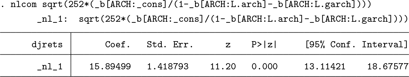
This increase in the value of the unconditional mean is also as expected given the effect of the crisis on return volatility.

The second point of interest is that the leverage parameter φ is once again negative and statistically significant. Furthermore, the size of the effect is approximately doubled from −0.0609 to −0.1240. The preponderance of bad news during the extended sample period appears to have magnified the leverage effect.

Finally, the estimate of the coefficient γ on the Treasury Bill rate in the GARCH(1,1)-X model is now found to be insignificant, even in the exponentiated specification adopted by Stata. This accords with intuition, because for a large part of this extended sample, short-term interest rates were at or near the 0 lower bound.

A plot of the annualized conditional volatility estimates over the sample period is given in figure 8. It is interesting to note how the peak of the conditional variance during the global financial crisis makes the previous peaks during the earlier sample around the dot-com bubble look rather modest.

Figure 8.

Estimated conditional volatility using a GARCH(1,1) model on the extended dataset, 23 August 1988–1 August 2017

Although no forecasting exercise is undertaken, the conditional variance is strongly mean reverting with an estimated HL of 47 days. This estimate is almost half of the estimate for the earlier sample and is indicative of a more powerful dynamic process for the conditional variance.

9 Conclusion

The aim of the original EP article was to characterize a volatility model in terms of its ability to forecast volatility and also to capture the stylized empirical facts about conditional volatility. Their article succeeds in doing this and also provides an accessible and useful introduction to volatility modeling. In terms of reproducibility, the results reported by EP stand up well to scrutiny and bring out some differences that prompt thought, particularly with respect to computing standard errors in GARCH models. Interestingly, the GARCH(1,1) model fit on updated data is very similar in terms of coefficient estimates, although the conditional variance process appears to be substantially less persistent when estimated over the longer sample. The model performs well in capturing the volatility around the global financial crisis and the turbulence in the markets during that period.

10 Programs and supplemental materials

Supplemental Material, sj-zip-1-stj-10.1177_1536867X211025797 - “What good is a volatility model?” A reexamination after 20 years

Supplemental Material, sj-zip-1-stj-10.1177_1536867X211025797 for “What good is a volatility model?” A reexamination after 20 years by Christopher F. Baum and Stan Hurn in The Stata Journal

Footnotes

10 Programs and supplemental materials

To install a snapshot of the corresponding software files as they existed at the time of publication of this article, type

Notes

References

Bollerslev

1986. Generalized autoregressive conditional heteroskedasticity. Journal of Econometrics 31: 307–327. https://doi.org/10.1016/0304-4076(86)90063-1.

Bollerslev

Wooldridge

J. M.

. 1992. Quasi-maximum likelihood estimation and inference in dynamic models with time-varying covariances. Econometric Reviews 11: 143–172. https://doi.org/10.1080/07474939208800229.

Brooks

Burke

S. P.

. 2003. Information criteria for GARCH model selection. European Journal of Finance 9: 557–580. https://doi.org/10.1080/1351847021000029188.

Diebold

F. X.

1986. Modeling the persistence of conditional variances: A comment. Econometric Reviews 5: 51–56. https://doi.org/10.1080/07474938608800096.

Drost

F. C.

Nijman

T. E.

. 1993. Temporal aggregation of GARCH processes. Econometrica 61: 909–927. https://doi.org/10.2307/2951767.

Engle

R. F.

1982. Autoregressive conditional heteroscedasticity with estimates of the variance of United Kingdom inflation. Econometrica 50: 987–1007. https://doi.org/10.2307/1912773.

Engle

R. F.

Bollerslev

. 1986. Modelling the persistence of conditional variances. Econometric Reviews 5: 1–50. https://doi.org/10.1080/07474938608800095.

Engle

R. F.

Patton

A. J.

. 2001. What good is a volatility model? Quantitative Finance 1: 237–245. https://doi.org/10.1088/1469-7688/1/2/305.

Fama

E. F.

1970. Efficient capital markets: A review of theory and empirical work. Journal of Finance 25: 383–417. https://doi.org/10.2307/2325486.

10.

Glosten

L. R.

Jagannathan

, and Runkle

D. E.

. 1993. On the relation between the expected value and the volatility of the nominal excess return on stocks. Journal of Finance 48: 1779–1801. https://doi.org/10.1111/j.1540-6261.1993.tb05128.x.

11.

Gould

Pitblado

, and Poi

. 2010. Maximum Likelihood Estimation with Stata. 4th ed. College Station, TX: Stata Press.

12.

Hansen

P. R.

Lunde

. 2005. A forecast comparison of volatility models: Does anything beat a GARCH(1,1)? Journal of Applied Econometrics 20: 873–889. https://doi.org/10.1002/jae.800.

13.

Lumsdaine

R. L.

1996. Consistency and asymptotic normality of the quasi-maximum likelihood estimator in IGARCH(1,1) and covariance stationary GARCH(1,1) models. Econometrica 64: 575–596. https://doi.org/10.2307/2171862.

14.

Martin

Hurn

, and Harris

. 2013. Econometric Modelling with Time Series: Specification, Estimation and Testing. New York: Cambridge University Press.

15.

Nelson

D. B.

1991. Conditional heteroskedasticity in asset returns: A new approach. Econometrica 59: 347–370. https://doi.org/10.2307/2938260.

16.

Zakoian

J.-M.

1994. Threshold heteroskedastic models. Journal of Economic Dynamics and Control 18: 931–955. https://doi.org/10.1016/0165-1889(94)90039-6.

17.

Zivot

2009. Practical issues in the analysis of univariate GARCH models. In Handbook of Financial Time Series, ed. Andersen

T. G.

Davis

R. A.

Kreiß

J.-P.

Mikosch

, 113–155. Berlin: Springer. https://doi.org/10.1007/978-3-540-71297-8_5.

Supplementary Material

Please find the following supplemental material available below.

For Open Access articles published under a Creative Commons License, all supplemental material carries the same license as the article it is associated with.

For non-Open Access articles published, all supplemental material carries a non-exclusive license, and permission requests for re-use of supplemental material or any part of supplemental material shall be sent directly to the copyright owner as specified in the copyright notice associated with the article.

0.08 MB

0.00 MB