Estimation of marginal effects for models with alternative variable transformations

Abstract

margins is a powerful postestimation command that allows the estimation of marginal effects for official and community-contributed commands, with well-defined predicted outcomes (see predict). While the use of factor-variable notation allows one to easily estimate marginal effects when interactions and polynomials are used, estimation of marginal effects when other types of transformations such as splines, logs, or fractional polynomials are used remains a challenge. In this article, I describe how margins‘s capabilities can be extended to analyze other variable transformations using the command f_able.

1 Introduction

margins is a powerful postestimation command that was introduced in Stata 11, allowing the estimation of marginal effects for all official estimation commands and any community-contributed command with a properly defined predicted outcome program (see predict). As described in Williams (2012), margins, and its companion marginsplot (in Stata 12), provides a great tool for analyzing and providing meaningful information that is easier to interpret and describe. Furthermore, in combination with factor-variable notation, also introduced in Stata 11, margins also allows users to easily estimate marginal effects when interactions and polynomials of continuous variables, and interactions with discreet variables, are used without any additional work from the user.

Despite these features, the ability of margins to estimate marginal effects is limited to the use of simple polynomials and interactions. Unless further information is provided to a command, Stata cannot identify the possible interdependencies across explanatory variables.

To the best of my knowledge, there are only two commands where this limitation is not binding. As described in Poi (2011), nl can be used to obtain marginal effects when using functions other than interactions of polynomials, even when the model is nonlinear in parameters, but assuming an additive error. npregress series, one of the newest additions to Stata 16 nonparametric analysis, also estimates marginal effects of arbitrary transformations of the independent variables (splines, B-splines, and polynomials), based on numerical derivatives. Unfortunately, both models are based on least-squares types of estimators. Neither command can be used in the case of nonlinear models like logit or probit. In the case of npregress series, users cannot freely choose what transformations to use. The only other program that proposes a strategy that may allow obtaining marginal effects, more specifically marginal means, using transformed covariates, was proposed by Royston (2013). His command, marginscontplot, uses a predefined mapping between original and transformed covariates to appropriately handle the constructed variables in margins.

This article describes a simple strategy, implemented by f_able, that allows the estimation of marginal effects of a larger set of nonlinear transformations using margins and the option nochainrule[numerical noestimcheck]. Section 2 provides a review of how marginal effects should be estimated, with emphasis on some of the computational challenges that are bypassed by the use of factor notation. Section 3 provides a simple approach for the estimation of marginal effects for the case of Spline regressions and compares it with a simplified case using npregress series. Section 4 introduces three commands that prepare the data for the estimation of marginal effects for any arbitrary variable transformation and shows how f_able can be used to estimate marginal effects using any variable transformation. Section 5 concludes.

2 Marginal effects: Theoretical approach

Marginal effects are useful statistics to measure the impact of a change that the independent variables will have on the dependent variable, assuming other covariates remain constant. At the beginning of most introductory econometric courses, very little emphasis is placed on understanding this concept because, for linear regressions, marginal effects are typically equal to the coefficient associated with the variable analyzed. Consider the following linear regression model:

$y_i=b_0+b_1{x}_{1i}+b_2{x}_{2i}+e_i$

1

Under the standard assumptions of exogeneity, homoskedasticity, and correct model specifications (see Wooldridge [2013]), the coefficients of (1) can be estimated using ordinary least squares (OLS). Under the ceteris paribus assumption, the marginal effect of x ₁ and x ₂ on y could be estimated based on the thought experiment of what would the outcome y_i be if x _{1 i} (x _{2 i} ) increases in one unit, keeping everything else constant. Mathematically, this is equivalent to obtaining the partial derivative of y_i with respect to x _{1 i} , which for (1) is given by b ₁ (b ₂):

$\text{Δ}{y}_i=\text{Δ}{x}_i{b}_1\to \frac{\text{Δ}{y}_i}{\text{Δ}{x}_{1i}}=\frac{\partial y_i}{\partial x_{1i}}=b_1;\hspace{1em}\frac{\partial y_i}{\partial x_{2i}}=b_2$

However, if we lift the homoskedasticity assumption, it is more convenient to estimate marginal effects using the conditional expectation assumption. Under this assumption, we estimate the average effect of a one-unit change in x ₁ or x ₂ across all individuals with the same observed characteristics (conditioning on x):

$\begin{array}{c}E\left(y_i\mid x\right)=b_0+b_1{x}_1+b_2{x}_2\\ \frac{\partial E\left(y_i\mid x\right)}{\partial x_1}=b_1;\hspace{1em}\frac{\partial E(y\mid x)}{\partial x_2}=b_2\end{array}$

This implies that for a simple linear regression [like (1)], where each variable appears only once, and without any transformation, marginal effects are directly identified by the estimated coefficients.

Later in a semester, students are introduced to the idea that nonlinear transformations and interactions of the independent variables can be included in the linear regression model. Because the model is still linear in parameters, it can be estimated using OLS. However, additional care needs to be taken when estimating the marginal effects because one needs to account for the interdependence of variable transformations. Consider the following model, with its conditional expectation form:

$\begin{array}{c}{y}_i=b_0+b_1{x}_{1i}+b_2{x}_{1i}^2+b_3{x}_{2i}+b_4{x}_{1i}{x}_{2i}+e_i\\ E\left(y_i\mid x\right)=b_0+b_1{x}_1+b_2{x}_1^2+b_3{x}_2+b_4{x}_1{x}_2\end{array}$

2

In this model, the marginal effect of x ₁ on y is no longer a constant, and it now depends on the values x ₁ and also of x ₂. Using calculus, the marginal effects for x ₁ and x ₂ in this model are

$\frac{\partial E\left(y_i\mid x\right)}{\partial x_1}=b_1+2b_2{x}_1+b_4{x}_2;\hspace{1em}\frac{\partial E\left(y_i\mid x\right)}{\partial x_2}=b_3+b_4{x}_1$

Because marginal effects are now functions of x ₁ and x ₂, one usually needs to decide what values of x ₁ and x ₂ to use when reporting marginal effect. Alternatively, one can also estimate marginal effects for all observed (or feasible) combinations of x ₁ and x ₂ and summarize (or plot) those estimates as needed. ¹ The standard practice is presenting average marginal effects (AME) or the marginal effects at the mean (MEM). For (2), they both will be the same:

$\begin{array}{ll}\text{AME}\hfill & \text{MEM}\hfill \\ E\left(\frac{\partial E\left(y_i\mid x\right)}{\partial x_1}\right)\hfill & {\frac{\partial E\left(y_i\mid x\right)}{\partial x_1}|}_{x=\overline{x}}=b_1+2b_2{\overline{x}}_1+b_4{\overline{x}}_2\hfill \\ E\left(\frac{\partial E\left(y_i\mid x\right)}{\partial x_2}\right)\hfill & {\frac{\partial E\left(y_i\mid x\right)}{\partial x_2}|}_{x=\overline{x}}=b_3+b_4{\overline{x}}_1\hfill \end{array}$

With this information, and assuming x ₁ and x ₂ are nonstochastic, standard errors associated with these marginal effects can be estimated, ² and the technical part of the analysis would be done.

The challenge with most software (including Stata) is that, unless additional information is provided, the software may not recognize that some variables are interrelated by construction and that the assumption of “everything else remaining constant” is incorrect. In the case of Stata, until factor variables were introduced, it could not automatically adjust for these interrelations, providing incorrect estimations of marginal effects, unless further steps were considered. Stata still fails to grasp these interrelations when we step beyond simple interactions or polynomials.

3 Marginal effects: Empirical approach

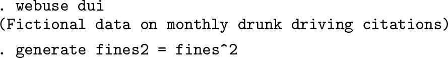
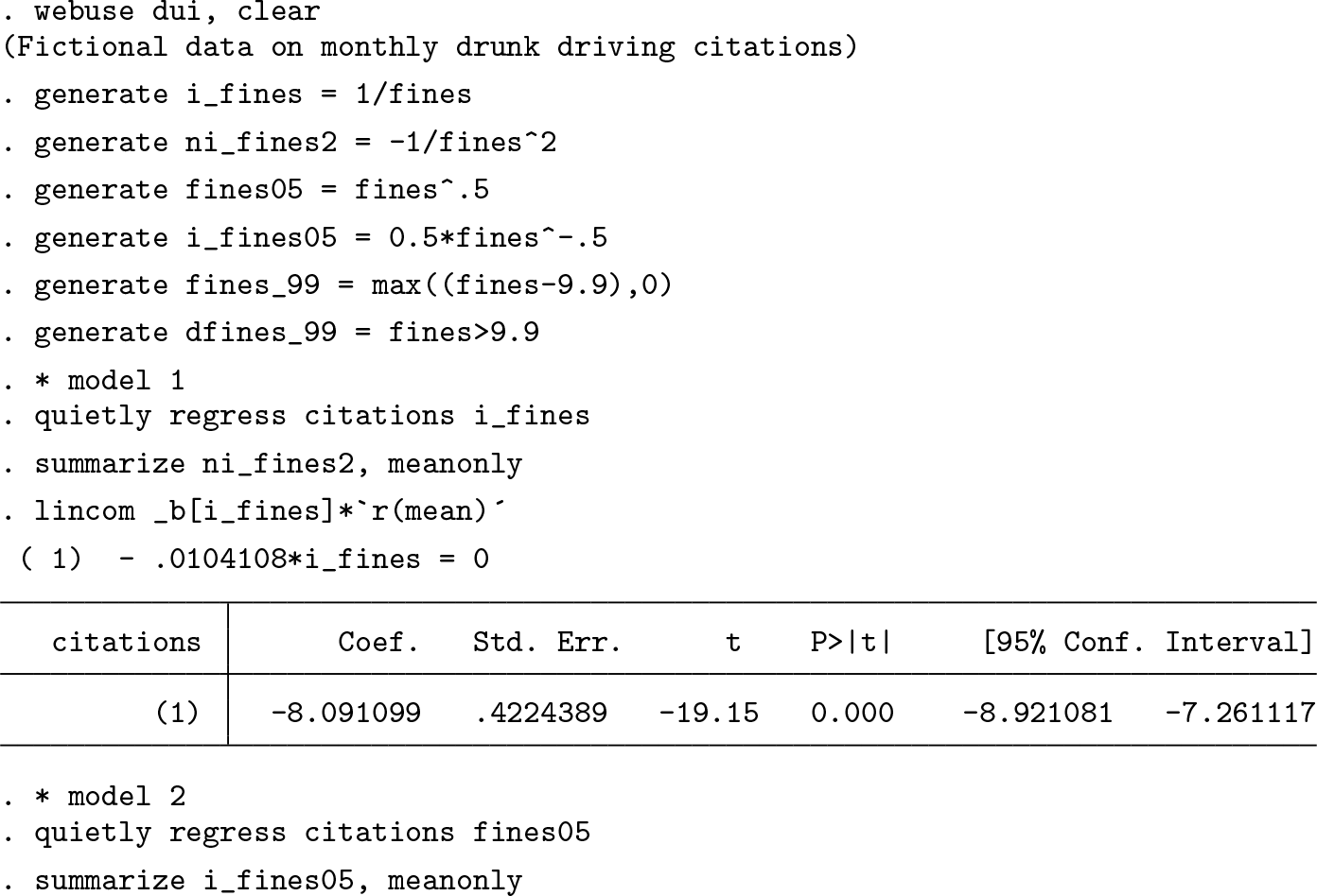
For this section, dui.dta, which is freely available online will be used. Consider the following model:

${\text{citations}}_i\text{ = }{b}_{\text{0}}\text{ + }{b}_{\text{1}}{\text{fines}}_i\text{ + }{b}_{\text{2}}{\text{fines}}_i^2\text{+ }{e}_i$

3

Before Stata 11 and factor notation, to fit a model like this, one would need to create all variables before including them in the model. For example, one would need to create a variable named fines2 to be equal to ${fines}_i^2$ ,

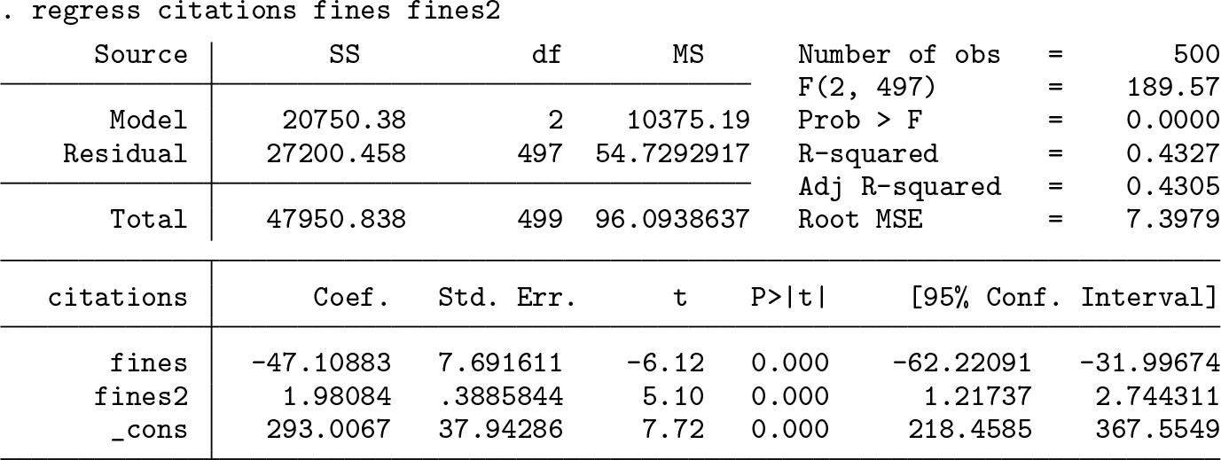
and fit the model using the command regress:

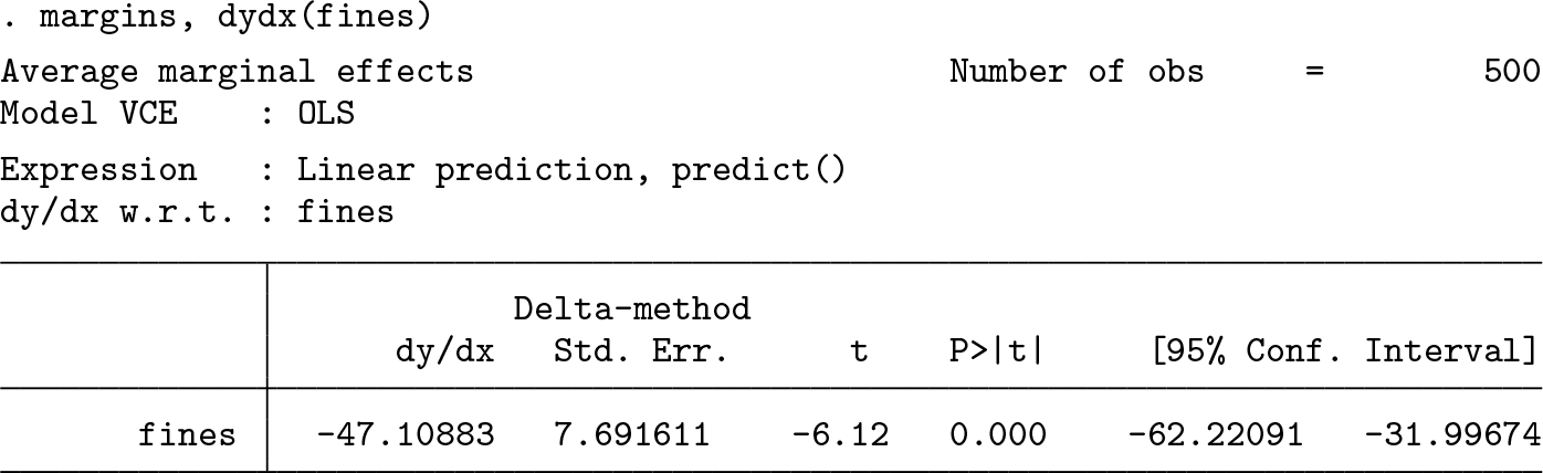
Using margins to calculate the marginal effects of fines on citations would produce the wrong answer because fines2 would not be handled correctly: there is no way for Stata to know that fines2 = fines ².

However, AME can be derived by hand by taking the derivative of (3) with respect to fines, using the average value of fines as the point of reference, and using lincom to calculate the marginal effects and standard errors:

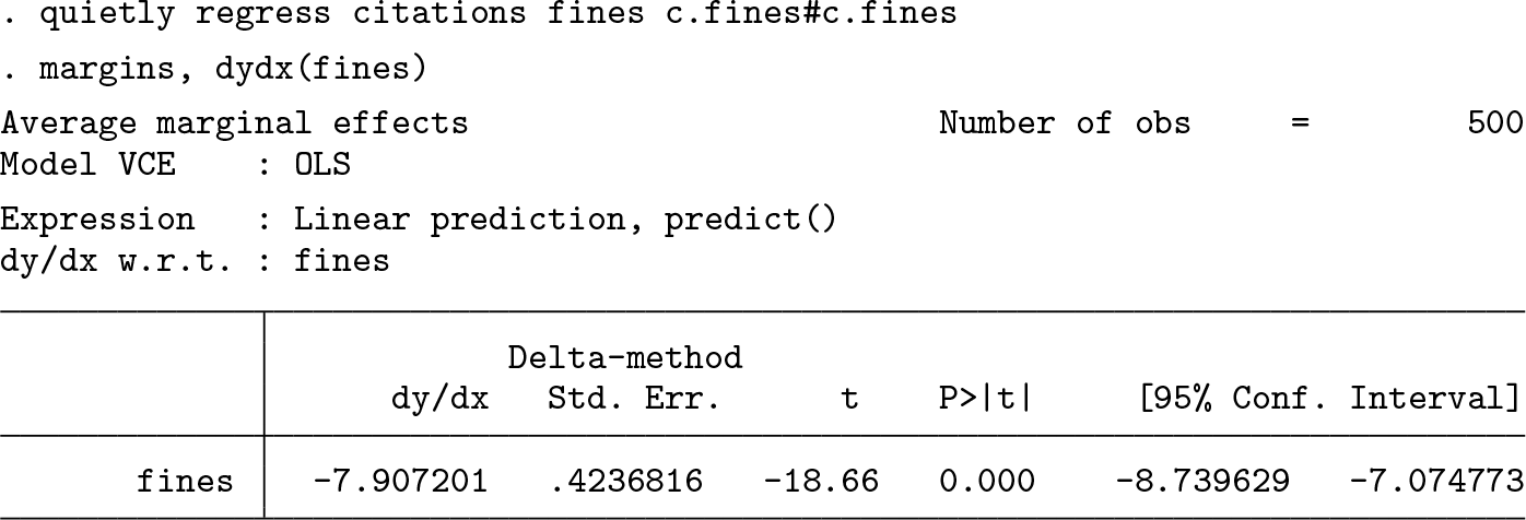
Since the introduction of Stata 11, estimating marginal effects for a model like this is much simpler. Using factor notation, we add the squared parameter and let margins handle the interaction on its own:

I suspect that the methodology behind the code for margins and factor notation “taught” Stata how to take derivatives of polynomials. In other words, Stata recognizes that when there is an expression like c. var1 #c. var1, it internally “knows” the analytical derivative is 2 × c. var1. Thus, margins simply uses this information to handle the squared parameter (c.fines#c.fines) before providing you with the result.

While this has been a big improvement for a better understanding of marginal effects, it does have its limitations. For example, margins would not be able to estimate marginal effects for the following models:

$\begin{array}{l}\text{ Model }1:{\text{ citations}}_i=b_0+b_1\left(1/{\text{fines}}_i\right)+e_i\hfill \\ \text{ Model }2:{\text{ citations}}_i=b_0+b_1{\text{fines }}_i^{0.5}+e_i\hfill \\ \text{ Model }3:{\text{ citations }}_i=b_0+b_1\text{fines }+b_2\max (\text{fines}-9.9,0)+e_i\hfill \end{array}$

4

However, mathematically, the AME, and MEM, can be derived directly using the sample means:

$\begin{array}{lll}\hspace{0.17em}\hfill & \text{AME}\hfill & \text{MEM}\hfill \\ \text{Model 1:}\hfill & b_1{n}^{-1}\sum \left(-\frac{1}{{\text{fines}}_i^2}\right)\hfill & -b_1\frac{1}{{\left(n^{-1}\sum {\text{fines}}_i\right)}^2}\hfill \\ \text{Model 2:}\hfill & 0.5\times b_1{n}^{-1}\sum \left({\text{fines }}_i^{-0.5}\right)\hfill & 0.5\times b_1{\left(n^{-1}\sum {\text{fines }}_i\right)}^{-0.5}\hfill \\ \text{Model 3:}\hfill & b_1+b_2{n}^{-1}\sum \left\{1\left({\text{fines}}_i>9.9\right)\right\}\hfill & b_1+b_2\times 1\left\{\left(n^{-1}\sum {\text{fines}}_i\right)>9.9\right\}\hfill \end{array}$

Which can be used to estimate the AME by hand. Now, concentrate on the estimation of the AME:

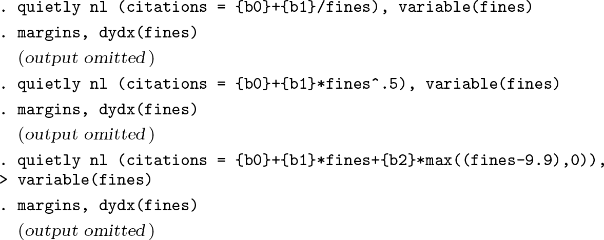
For these models, one also has the option of using nl to estimate the marginal effects, which requires less work: ³

This flexibility of nl to estimate marginal effects with nonstandard transformations motivates the following question: why can nl “correctly” estimate marginal effects, whereas regress cannot? The answer is rather simple: we are not using a constructed variable in the model; instead, we are using the original variable and allowing nl to construct the new variable.

This means that, while we see this model is being fit,

what may be happening in the background is different. Stata identifies which elements of this code are parameters to be estimated (those within brackets) and which elements need to be created (fines.⁵) before fitting the model. In other words, Stata is estimating the following:

Here __000000 is a temporary variable that was constructed as fines ^.5 and that you never see. The difference is that nl knows that __000000 = fines ^.5.

How is it that nl knows that the derivative of fines ^0.5 is 0.5fines ^−0.5? The answer is nl does not know. The only type of analytical derivatives Stata may know is when interactions are used, specifically factor notations. However, because Stata “remembers” how a variable was constructed, it can use numerical derivatives to make a reasonable approximation for the analytical derivative.

For example, the numerical derivative for the transformation fines ^{0 .5} can be approximated as follows:

$\frac{\partial ({\text{fines}}^{0.5})}{\partial \text{fines }}=\frac{{(\text{fines }+h)}^{.5}-{(\text{fines }-h)}^{.5}}{2h}\text{ for a sufficiently small }h$

This expression is surprisingly accurate. ⁴ For this example, when h = 1, the largest absolute difference between the numerical and analytical derivative is 0.000423, whereas when h = 1/216, the largest difference is 6.58e–09. This implies that margins does not need to know how to obtain analytical derivatives, because it can use numerical derivatives instead and use this information to estimate the appropriate marginal effects.

4 f_able: Marginal effects for arbitrary variable transformations

The previous sections described how marginal effects should be estimated and how to use that information to obtain AME or MEM by comparing the step-by-step procedure with what margins does. They also detailed how nl can estimate marginal effects for variable transformations other than interactions using numerical derivatives to approximate the analytical derivatives. This implies that Stata already has the capability to estimate marginal effects when transformations other than interactions and polynomials are used in a model. However, to expand those capabilities to any linear and nonlinear model, we need to “tell” Stata that some variables are based on constructions from others so that Stata can use this information to correctly estimate marginal effects.

In this section, I first sketch the basic structure of the programs required to solve this problem and then describe the commands within f_able that address this problem.

4.1 f_able: Basics

One solution to pass information about variable dependencies to Stata is to use the variable label to “store” the transformation used to create the variable of interest. To automate this procedure, I propose two small programs that “wrap” around Stata’s built-in commands generate and replace:

These two commands have one purpose: when a new variable is created, it will label it with the expression used to create it, and if the values are replaced, it will change the label to the new expression used.

Consider model 3 from (4). The variable of interest can be created using the command fgen, but I created it with an intentional mistake:

However, I can rectify it using the command frep and replace the values fines2 with the correct content:

In addition to setting up the data for the next step of the estimation of marginal effects, these commands may be useful for tracking how variables are created or modified.

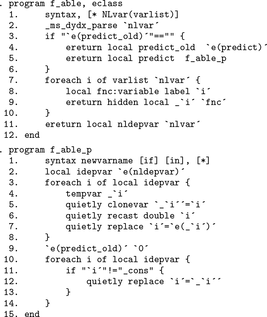
The second step is to explicitly tell Stata that a particular variable is constructed based on other variables in the model and that when margins is called, the constructed variable needs to be updated every time the original variable changes. This can be done with the two following programs:

The first program, f_able, does three things. First, it adds information to any previously fit model indicating which variables are constructed variables using e(nldepvar). Second, it adds hidden macros with information regarding the data transformation used. ⁵ Last, it redirects predict from the original e(predict) command to the one defined below as f_able_p but keeps the original information in e(predict_old).

The second program, f_able_p, has only one purpose—updating the constructed variables identified in e(nldepvar)—before obtaining the predicted values appropriate for the estimated command e(predict_old), using the information previously stored in the hidden macros.

With these two pieces of code, the last step is to call margins for the estimation of the marginal effects, using the option nochainrule. ⁶ This is an option often overlooked when using official Stata commands. However, as its help file indicates, “nochainrule is safer because it makes no assumptions about how the parameters and covariates join to form the response.”

This implies that when a model like the following is fit,

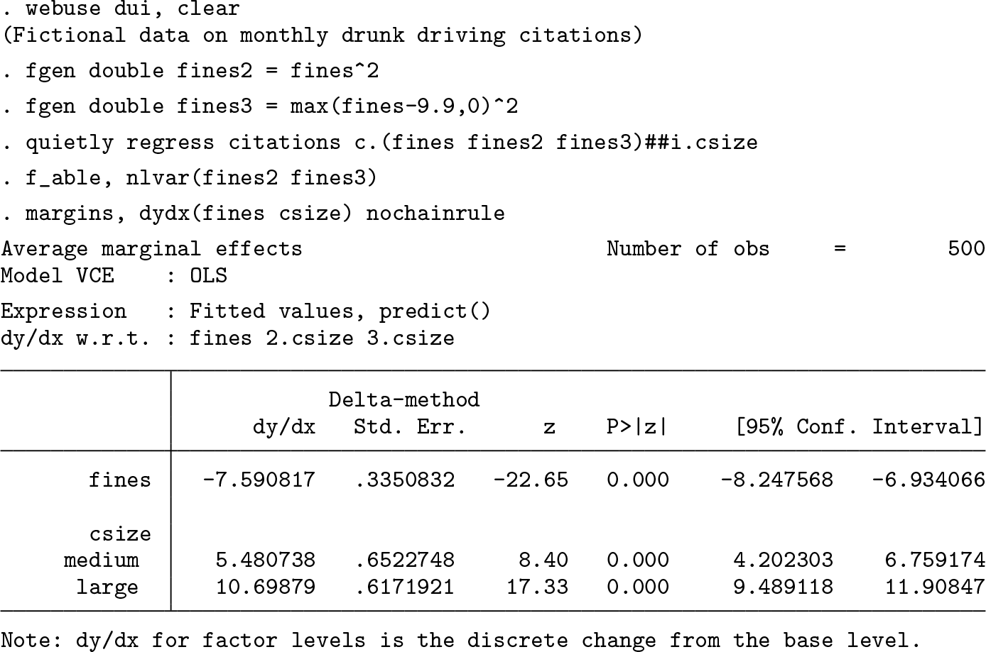
marginal effects will be calculated using the coefficient of fines and the coefficient of fines2 times the numerical derivative of fines2 with respect to fines, if fines2 was declared as a constructed variable. Let see how this works.

The first line fits the model with citations as a dependent variable and fines and fines2 as independent variables. fines2 is the one we defined previously as max(fines − 9.9, 0). The second line calls f_able to identify that fines2 is a constructed variable, and the last step estimates the marginal effects using nochainrule. The results are the same as those done by hand or those using the nl command. They can also be replicated using npregress series.

Notice that while the point estimates are the same, the standard errors produced by npregress series are somewhat larger than those produced with nl or with the proposed strategy, because npregress reports robust standard errors by default.

We can also compare the output of f_able with the output we could obtain using factor notation:

This method replicates the results when using factor notation up to five decimal places, but some degree of precision is lost because of forced use of numerical derivatives.

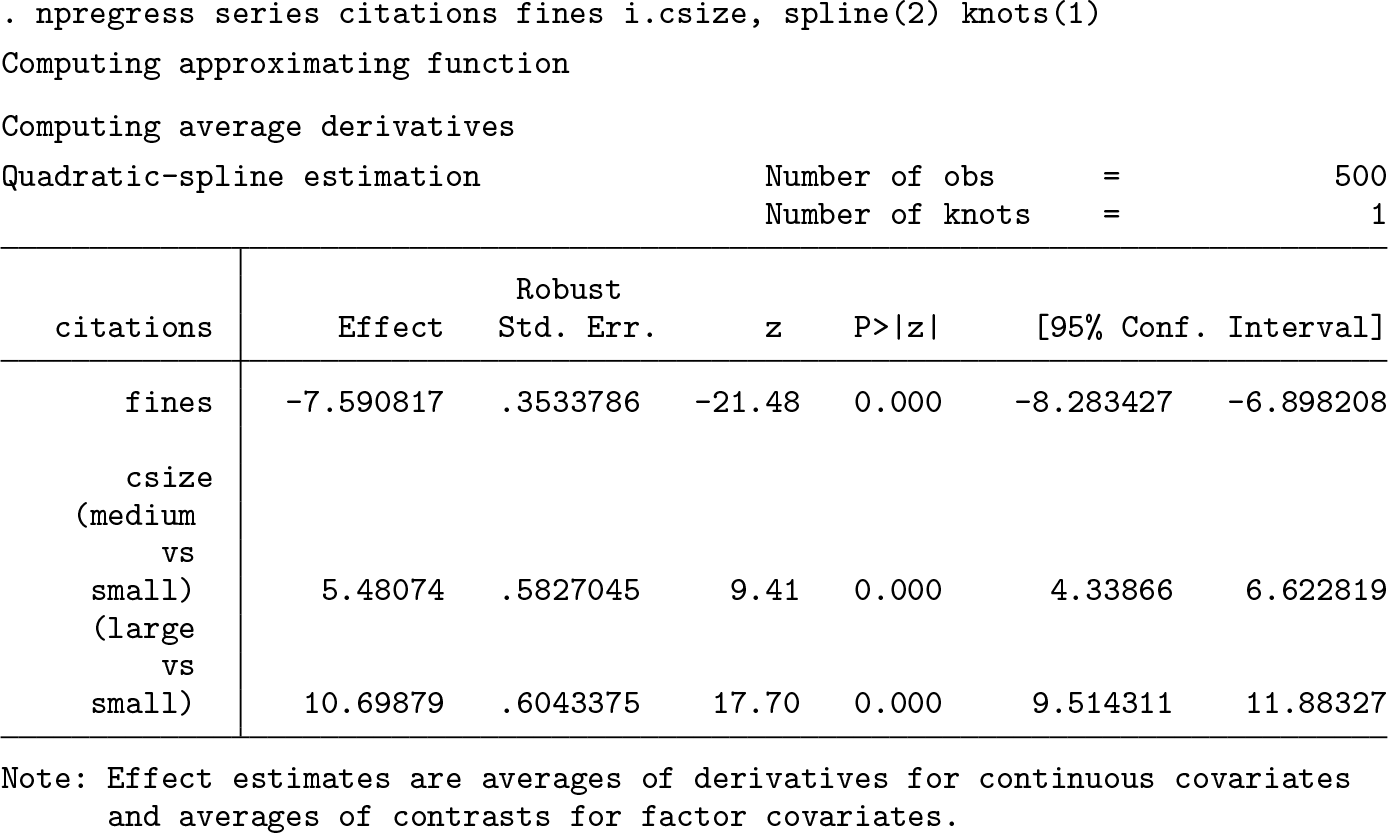
Last, here is a more challenging estimation that combines the use of factor notation with f_able and compares the output with that of the npregress series.

The same can be replicated using regress and f_able:

Once again, this replicates the output with very small differences in the point estimates but with some differences in terms of the standard errors, because npregress reports robust standard errors.

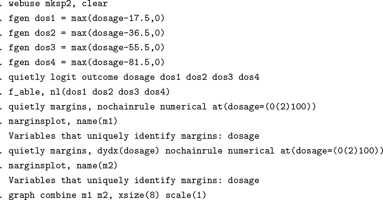
We can also use this strategy for models other than OLS. Consider mksp2.dta. As with the example provided in the help file for the command mkspline, four variables are created to allow for linear splines with four knots. A logit model of the outcome against dosage is fit, and the constructed variables are estimated. margins needs to include the options nochainrule and numerical. The predicted probabilities and the marginal effects across various values of dosage are produced:

Figure 1.

Predicted probabilities and marginal effects

4.2 f_able package

In the previous subsection, I sketched the basic code that can be used to store information in regression outputs so that it can be used by margins to estimate marginal effects after most linear and nonlinear models. In this subsection, I describe all the programs that are part of f_able and can be used to address some limitations of the strategy.

fgen newvar = exp

frep oldvar = exp

fgen and frep can be used to create a new variable or replace an existing variable using any expression that is valid with generate. fgen creates a variable in double format to reduce problems of precision with the constructed variables. If the expression is longer than 75 characters, it assigns the label See note, and a variable note will store the used expression.

f_able, nlvar( varlist )

f_able is used to declare which variables in the model specification should be considered as “constructed” variables. All variables in nlvar(), which should be present in the previous model specification, are stored in a macro named e(nldepvar). After one uses f_able, marginal effects with respect to the constructed variables are no longer possible unless f_able_reset is used. A list of hidden macros named e(_varname) is also stored and contains the information of how each variable (varname) was created.

f_able_reset restores all the postestimation results to the state previous to using f_able.

f_symev and f_symrv are commands that force the variance–covariance matrices stored in e(V) and r(V), respectively, to be symmetric when a nonsymmetric warning appears. The warning appears because of the precision loss and forced numerical derivatives, which creates variance–covariance matrices that are nonsymmetric. This often occurs after using margins for multiple points of reference.

5 Conclusion

This article describes how marginal effects can be estimated using analytical derivatives, as well as numerical derivatives. It introduced two small programs, within the f_able package, that enable margins to estimate marginal effects when using transformations beyond variable interactions and polynomials.

These commands can be used to estimate marginal effects for many official Stata commands as well as other community-contributed commands that can produce sensible predicted outcomes. The strategy does have three limitations: first, the estimated marginal effects depend on the precision of the forced numerical derivatives; second, it requires the original variable to be present in the model specification so that marginal effects can be used; and third, because f_able is forcing margins to do something it is not meant to do, one may experience difficulties estimating marginal effects and standard errors when the request is particularly complex.

While the limitation regarding the precision of the estimates is unavoidable, the other limitations can be circumvented to some extent. In the second limitation, the original variable can be added to the list of explanatory variables using o.. This omits the original variable from the estimation but keeps it in the list of explanatory variables, allowing the estimation of margins.

The last limitation can be addressed with careful troubleshooting. While the option nochainrule forces margins to use numerical derivatives for the estimation of marginal effects after most commands, some commands such as probit, logit, and poisson require using the options nochainrule and numerical. If point estimates appear as missing, the option noestimcheck can be used to bypass some of the safety checks in margins that produce this error. Finally, if standard errors are missing when estimating marginal effects for multiple points of interest, it may be because the estimated variance–covariance matrix created after margins is nearly symmetric. For those cases, f_symev and f_symrv can be used to force symmetry on the variance–covariance matrix produced by margins, so one can report standard errors or plot confidence intervals after marginsplot.

Supplemental Material

Supplemental Material, sj-zip-1-stj-10.1177_1536867X211000005 - Estimation of marginal effects for models with alternative variable transformations

Supplemental Material, sj-zip-1-stj-10.1177_1536867X211000005 for Estimation of marginal effects for models with alternative variable transformations by Fernando Rios-Avila in The Stata Journal