Effect sizes for contrasts of estimated marginal effects

Abstract

The statistical literature is replete with calls to report standardized measures of effect size alongside traditional p-values and null hypothesis tests. While effect-size measures such as Cohen’s d and Hedges’s g are straightforward to calculate for t tests, this is not the case for parameters in more complex linear models, where traditional effect-size measures such as η ² and ω ² face limitations. After a review of effect sizes and their implementation in Stata, I introduce the community-contributed command mces. This postestimation command reports standardized effect-size statistics for dichotomous comparisons of marginal-effect contrasts obtained from margins and mimrgns, including with complex samples, for continuous outcome variables. mces provides Stata users the ability to report straightforward estimates of effect size in many modeling applications.

1 Introduction

Classical frequentist statistical inference involves calculating p-values, or the probability that a null hypothesis would be observed in the target population given the data. It is well known that p-values are often misinterpreted as the probability that the null hypothesis is true (Cohen 1994). This widespread misunderstanding, combined with a raft of criticism admonishing both researchers and consumers that statistical significance does not imply clinical or practical significance, has led many voices in the field of statistics to encourage a move toward reporting standardized measures of effect size alongside or in place of traditional null hypothesis significance tests (for example, Kline [2013]; Trafimow and Marks [2015]; Wasserstein and Lazar [2016]; and Ziliak and Mc- Closkey [2008]). This article begins with a brief primer on standardized effect sizes and illustrates ways that they are traditionally estimated in Stata. Because the estimation of marginal effects is a core Stata capability, I review various ways of manually calculating effect sizes for margins results. These manual calculations are cumbersome, and in some cases impossible, using existing methods. Accordingly, I introduce a new command, mces, that facilitates computing contrasts of postestimation marginal effects for continuous outcome variables using margins. I then demonstrate its use with some of the same examples.

2 Overview of effect-size measures

While null hypothesis significance testing concerns whether “no effect is unlikely”, measures of effect size report whether an observed effect is “large in magnitude”. Because of differences in ways that effects are estimated, there can be no single way that effect sizes are calculated or reported. When researchers refer to “effect sizes”, they are almost always referring to standardized measures of effect size, which permit unit-neutral comparisons across studies and are a central tool of meta-analysis (Vacha-Haase and Thompson 2004). The literature frequently describes three “families” of effect sizes with similar properties, depending on the nature of the variables in question and the estimation procedure (Ellis 2010). While effect sizes are not infallible (for example, Cheung and Slavin [2016]), they are still preferable to reporting p-values alone because they report fundamentally different information (Kelley and Preacher 2012). While the terms “treatment group” and “control group” are the language of experimentation and are used in this article for exposition, the logic is the same for any binary demarcation of group membership, such as i.male or i.collgrad.

2.1 The “d” family of effect sizes

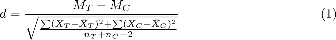
The “d” family reports magnitudes in terms of group mean differences. For continuous outcomes, these measures are variations on the generic formula (M_T − M_C )/SD: the mean difference between the treatment group and the control group, standardized by dividing by the standard deviation. The most familiar of these may be Cohen’s d (Cohen 1988), which involves dividing the differences in means by the pooled standard deviation (1):

$d=\frac{M_T-M_C}{\sqrt{\frac{{\displaystyle \sum {\left(X_T-{\overline{X}}_T\right)}^2}+{\displaystyle \sum {\left(X_C-{\overline{X}}_C\right)}^2}}{n_T+n_C-2}}}$

1

While Cohen’s d is likely familiar to readers, it is not the only statistic for standardized mean difference. Glass’s Δ (Glass, McGaw, and Smith 1981) reports the effect size using the standard deviation for the control group on the theory that this estimates average treatment effects for future untreated populations (2). It is also useful for small samples, when estimates of the standard deviation could be unstable.

$\Delta =\frac{M_T-M_C}{{\text{SD}}_C}$

2

Hedges’s g (Hedges 1981) uses a pooled standard deviation that is weighted by the relative sample sizes of the two groups (3). Hedges’s g is similar to Cohen’s d, but Cohen’s d has been shown to be positively biased in small samples.

$g=\frac{M_T-M_C}{\sqrt{\frac{{\text{SD}}_T^2\cdot \left(n_T-1\right)+{\text{SD}}_C^2\cdot \left(n_C-1\right)}{n_T+n_C-2}}}$

3

Hedges’s g and Cohen’s d are equivalent in large samples and will be similar to Glass’s Δ when the two groups have similar standard deviations.

2.2 The “r” family of effect sizes

In contrast to the “d” family’s emphasis on mean differences, the “r” family of effect-size measures revolves around the “proportion of variance accounted for”. The most familiar of these may be the squared multiple correlation coefficient (the “coefficient of determination”), or R ², and its “corrected” corollary, the adjusted R ², which incorporates information about sample size and number of predictors. These range in value from 0 to +1. While software traditionally reports R ² in regression analyses, with ANOVA “correlation index” values η ² and ω ² (sometimes ǫ ²) are more common, even though in linear relationships they are functionally equivalent to R ² and adjusted R ² (Cohen et al. 2003). Because they are measures of the proportion of variance accounted for, both R ² and η ² are figured by dividing the variance explained by the model (which may be as simple as a one-factor ANOVA or as complex as a structural equation model) by the total variance observed, as in (4).

$R^2\equiv {\eta }^2=\frac{{\text{SS}}_{\text{Model }}}{{\text{SS}}_{\text{Total }}}=\frac{\text{ Variance explained }}{\text{ Total variance }}$

4

Partial η ² and ω ², on the other hand, have a slightly different formula (5), which is comparable with (4) in a one-way ANOVA. However, in complex models, they can differ widely, and there is a great deal of published literature that appears to conflate the two (Levine and Hullett 2002). Readers may be expecting η ² and ω ² statistics to report the proportion of the “total” variance explained, as calculated in (4). Levine and Hullett recommended that partial η ² be reported, but other authors recommend the opposite (for example, Tabachnick and Fidell [2019] and Olejnik and Algina [2003]).

$\text{Partial }{\eta }^2\hspace{0.17em}=\hspace{0.17em}\frac{{\text{SS}}_{\text{Explained}}}{{\text{SS}}_{\text{Explained}}{\text{+ SS}}_{\text{Error}}}$

5

Use of measures such as η ² to report relative-effect magnitude has been criticized in the literature on regression (for example, Pedhazur [1997]). The standardized regression coefficient β is also occasionally advocated as an analogue to effect size, but it is not an ideal method to convey the magnitude of an effect across studies (Greenland et al. 1986; Pedhazur 1997).

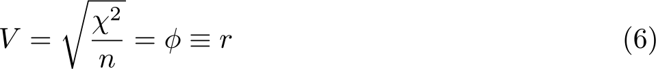
Effect sizes for categorical outcomes are also members of the “r” family. While they are related to r, more common measures of effect size for contingency tables (that is, categorical data) are coefficient φ, Cramér’s V, Kendall’s τ, and Cohen’s w. Equation 6 demonstrates the formula for these measures in a 2 × 2 table. While Cramér’s V can be calculated for multiway tables, φ is only estimated for two dichotomous variables, and Pearson’s r is only equivalent to V and φ in that case.

$V=\sqrt{\frac{{\chi }^2}{n}}=\varphi \equiv r$

6

Kendall’s τ is a nonparametric measure of association that does not use the χ ² statistic but rather ordinal “concordances” and “discordances”. There are three formulas for Kendall’s τ, according to whether the table is square and whether to account for ties. Stata reports Kendall’s τ_b , which is determined by the number of concordances (C), the number of discordances (D), the number of ties (T), and the number of observations (n), shown in (7).

${\tau }_b=\frac{C-D}{\sqrt{\left\{n(n-1)/\left(2-T_X\right)\right\}\left\{n(n-1)/\left(2-T_Y\right)\right\}}}$

7

Because the “d” and the “r” families are both undergirded by the same general linear model, they imply the same meaning, and researchers can use formulas to convert not only within families but also from one family to another (Vacha-Haase and Thompson 2004).

2.3 The “OR” family of effect sizes

Applied most commonly to categorical data and particularly generalized linear models, the odds ratio reports the odds of an outcome given a treatment or condition, relative to the odds of the outcome in the absence of that treatment or condition. Odds are figured from probabilities according to the formula π/(1 − π), where π is the probability of a “yes” result for a dichotomous outcome variable. ¹ Odds are accordingly the expected number of “yes” results for every “no”.

Odds ratios report magnitudes of association as a multiplier for the increase or decrease in odds for a one-unit change in a continuous predictor or, for categorical variables, membership in one category relative to another. For example, an odds ratio of 2 for a binary regression predictor variable i.urban implies that the odds of “yes” are twice as high for cities coded as urban as they are for those not coded as urban. Relative risk is an analogous standardized effect-size statistic measured in raw probabilities rather than odds. However, because relative risk has skewed sampling distributions, odds ratios are preferred in many fields.

3 Effect sizes in Stata

Stata has methods for estimating each family of effect-size measures. For an additional overview, see Huber (2013).

3.1 The “d” family in Stata

Stata’s base esize command reports “d” family effect sizes. The unequal option, which is generally recommended, requests that Stata use a pooled standard deviation rather than making the (strong) assumption that both groups have equal variances.

esize reports two values of Glass’s Δ, one using the standard deviation from the first group (“Glass’s Delta 1”, which is Domestic in this output) and one using the standard deviation from the second group (“Glass’s Delta 2”, which here is Foreign). In this example, Cohen’s d and Hedges’s g values are similar, ² while Glass’s Δ values are quite different, even though they all use the same M_C − M_T numerator. A closer examination of the sample statistics is instructive.

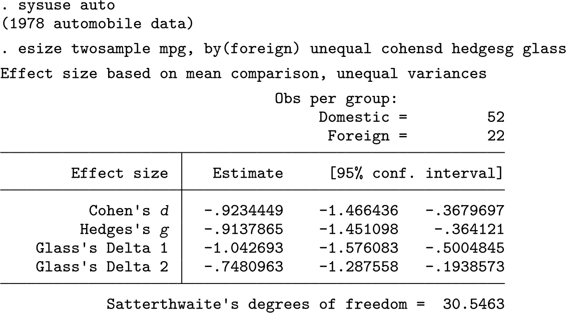
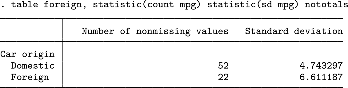
The standard deviations and sample sizes for the two groups are both different. After some algebra, we determine that the pooled unweighted standard deviation used for Cohen’s d is 5.36, while the pooled weighted standard deviation used for Hedges’s g is similar at 5.41. Both are closer to the Domestic standard deviation because the Domestic n is larger. The difference between SD_Domestic and SD_Foreign is responsible for the discrepancy between the two values of Glass’s Δ. In practice, the control group standard deviation will typically be closer to the population standard deviation, so the appropriate value of Δ is almost always the control group—in this case, “Glass’s Delta 1”.

3.2 The “r” family in Stata

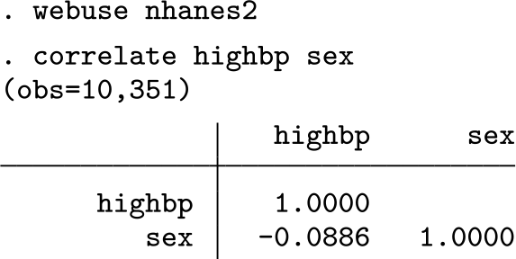
Stata provides several ways to estimate the “r” family of effect sizes. The correlate command and the related pwcorr command report the Pearson correlation coefficient,

which is the archetypal r. Coefficient r is equivalent to coefficient ϕ in a 2 × 2 table but is less often reported for contingency tables.

Coefficient ϕ, Cramér’s V, and Kendall’s τ are obtained in Stata with the tabulate twoway command. As expected, the value of r from the correlate command equals the estimated Cramér’s V because both variables are dichotomous.

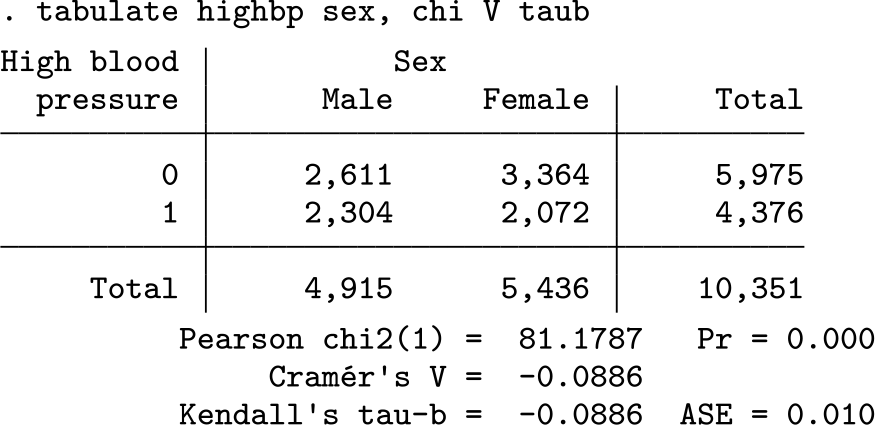
The χ ² test indicates statistical significance, but a small p-value is not an indication of how strongly these variables are associated with one another. The values of Cramér’s V and Kendall’s τ_b report that, on a scale from 0 (independence) to 1.0 (perfect association), sex’s association with the incidence of high blood pressure is less than 0.1. Coefficient ϕ is not reported, but in a 2 × 2, table it is equal to Cramér’s V. Here is another example, this time with a 2 × 5 table:

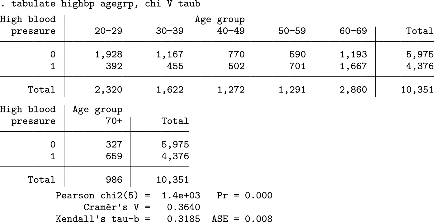
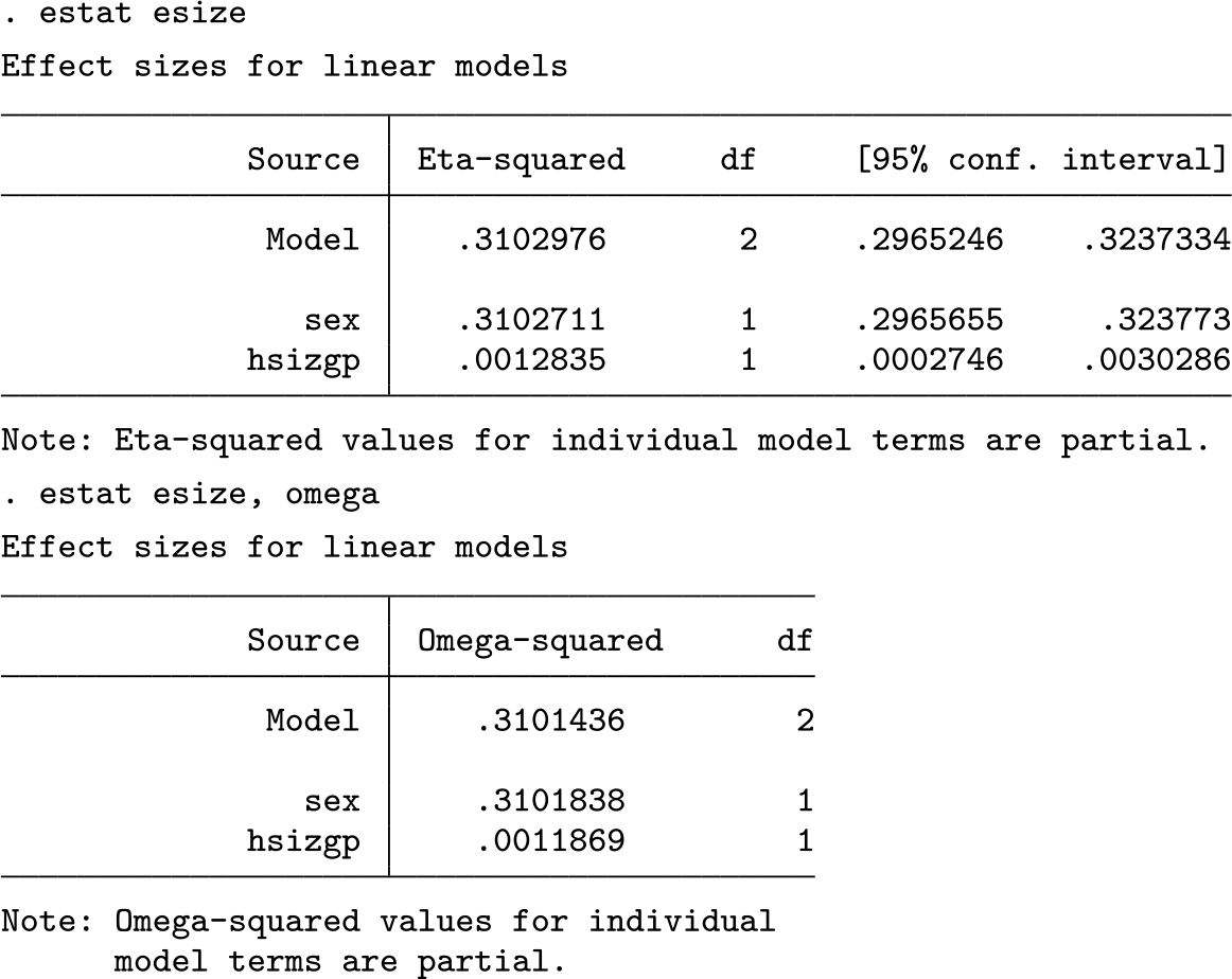
The p-value again leads us to reject the null hypothesis of no differences between the groups. Even though the tests for sex and age report p-values of 0.000, the estimated effect sizes show that age has a much stronger association with blood pressure than sex does. Taken together, these results underscore the importance of effect sizes in the interpretation of statistical test results, because without the effect sizes, the analyst could miss the critical differences in magnitude between the two associations.

Next we will consider the “r” family effect sizes in the context of linear models such as regression and analysis of variance. We begin with a simple regress specification (although typing anova hgb sex hsizgp is equivalent) followed by estat esize with and without the omega option.

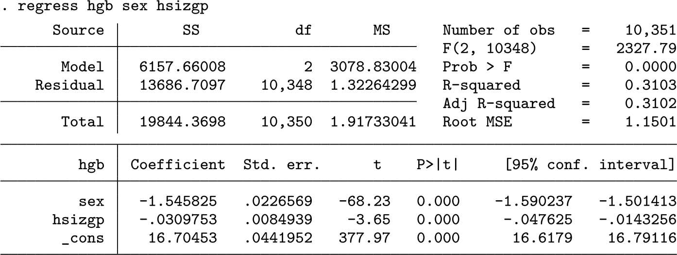
The value of R ² reported in the regression table is equivalent to η ², and the adjusted R ² is equivalent to ω ². In this instance with few predictors, η ² and ω ² (and R ² and adjusted R ²) are similar. They will diverge with the addition of more predictors.

The regress and anova commands report coefficients, t-values, and significance tests for each coefficient, along with R ² and adjusted R ², but only the postestimation estat size command reports η ² or ω ². These statistics can also be informative (compare Pedhazur [1997]). While both the sex and hsizgrp variables have p-values of less than 0.001 and are “statistically significant”, the partial ω ² shows that sex is much more strongly associated with hemoglobin levels when controlling for house size. In this instance, the t-values also suggest a difference in strength of association, but this is not always the case. The community-contributed command pcorr2 (Williams 2003) also reports partial correlation coefficients. In simple models, squared partial correlation coefficients from pcorr2 are equivalent to η ². Another community-contributed command, esizereg (Linden 2019), reports Cohen’s d effect sizes for a single regression coefficient.

3.3 The “OR” family in Stata

Odds ratios are most often calculated for logistic and ordered logistic regression models using logit or ologit. Because the default coefficients of these models are uninterpretable log odds, the or option requests exponentiated odds ratios instead, which facilitates interpretation. (The logistic command requests odds ratios by default, the same as logit, or.) Multinomial (also called “polytomous”) logistic regression models using mlogit with the rrr option report the similarly interpreted “relative-risk ratio”, and models for count outcomes, such as poisson and nbreg, calculate the “incidencerate ratio” with the irr option. As an example, consider a logistic regression analysis modeling risk factors for diabetes. The research question might be, “Do sex, age, or body mass index predict the likelihood of a person being diagnosed with diabetes?”

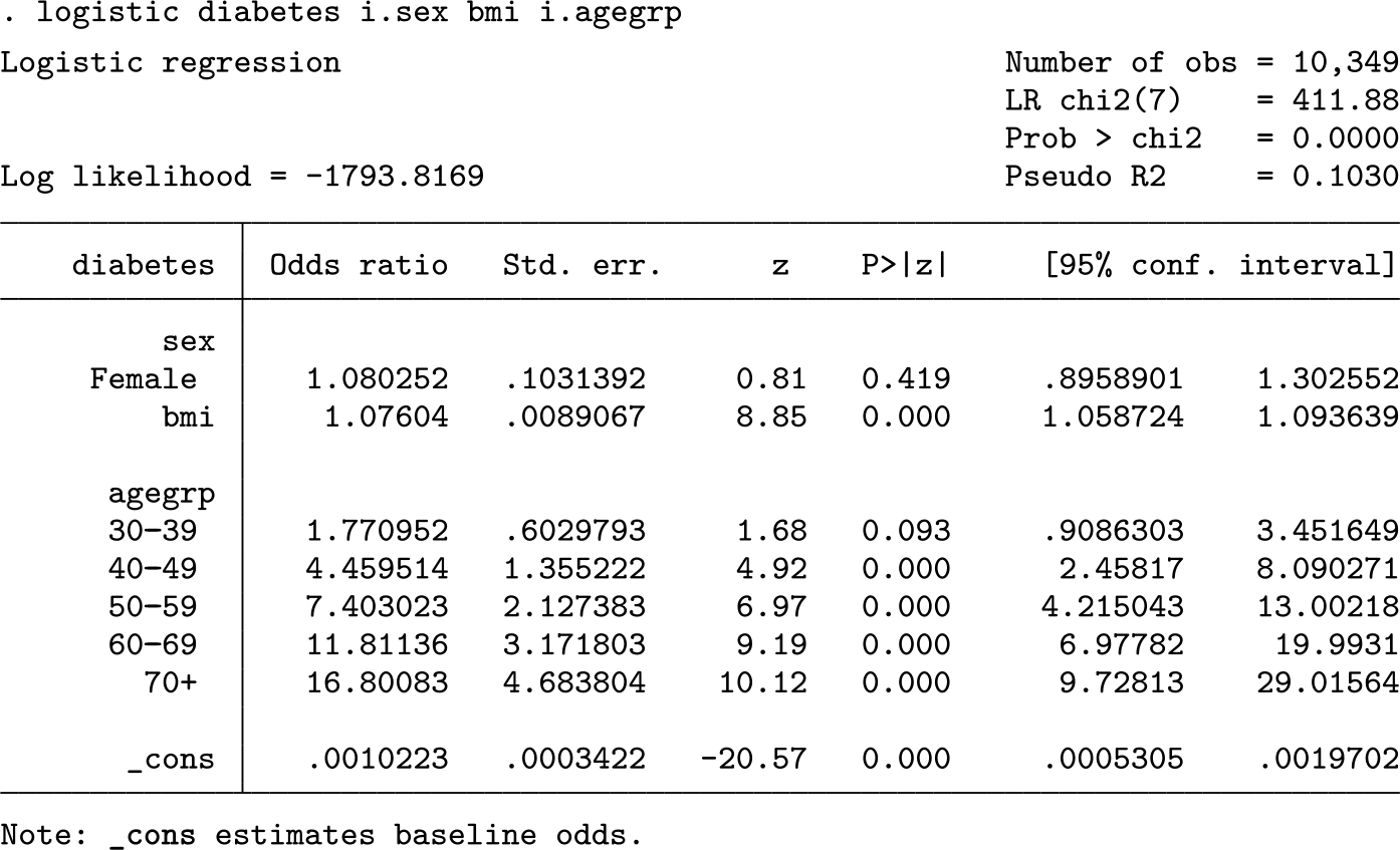
The model reports that females in the dataset have odds of being diagnosed with diabetes that are 1.08 times higher than males after controlling for the effects of the other predictors—not a huge difference. Critically, this is not the same as the “probability” of a diabetes diagnosis being 1.08 times higher. Odds use the formula π/(1 − π), and they are not linearly related to predicted probabilities. To obtain predicted probabilities, we use the margins command. Measures of effect size for regression models are elaborated further in the next section.

The coefficient for body mass index (BMI) also rounds to 1.08, but because BMI is a continuous predictor, the interpretation is that for each ceteris paribus one-unit increase in BMI, the odds of a diabetes diagnosis are expected to increase by a factor of 1.08, which would mean that a four-unit increase in BMI should predict odds of a diabetes diagnosis that are 1.36 times higher. And, relative to the base category of 20–29-yearolds, those aged 50–59 have odds of diabetes that are approximately 7.4 times higher. More information on odds ratios and their interpretations in Stata are available in Long and Freese (2014) and Mitchell (2021).

4 Effect sizes for marginal effects

The interpretation of regression coefficients is less straightforward when models become complex. When transformations, interactions, and polynomials are specified and combined, individual model coefficients can lose their clear, substantive meaning. Fortunately, as experienced Stata users know, the ability to easily calculate postestimation predicted values from even the most complicated models using the margins command is one of Stata’s core capabilities. Just as interpretation of regression coefficients becomes more difficult with increasing model complexity, so does the interpretation of the “r” family of effect sizes. While η ² and ω ² have straightforward interpretations in simpler models, they offer less clarity on the magnitude of a variable’s effects on the outcome when models become complex, especially without careful centering and hand calculations of “simple slopes” (Aiken and West 1991). η ² and ω ² values also do not leverage the flexible specifications of margins. The pwcompare option for margins can be used to produce the M_T − M_C component of the formula for the “d” family of effect sizes with many types of regression models. However, as we shall see, calculating a valid standard deviation can be a challenge.

4.1 Marginal effect sizes for categorical regression predictors

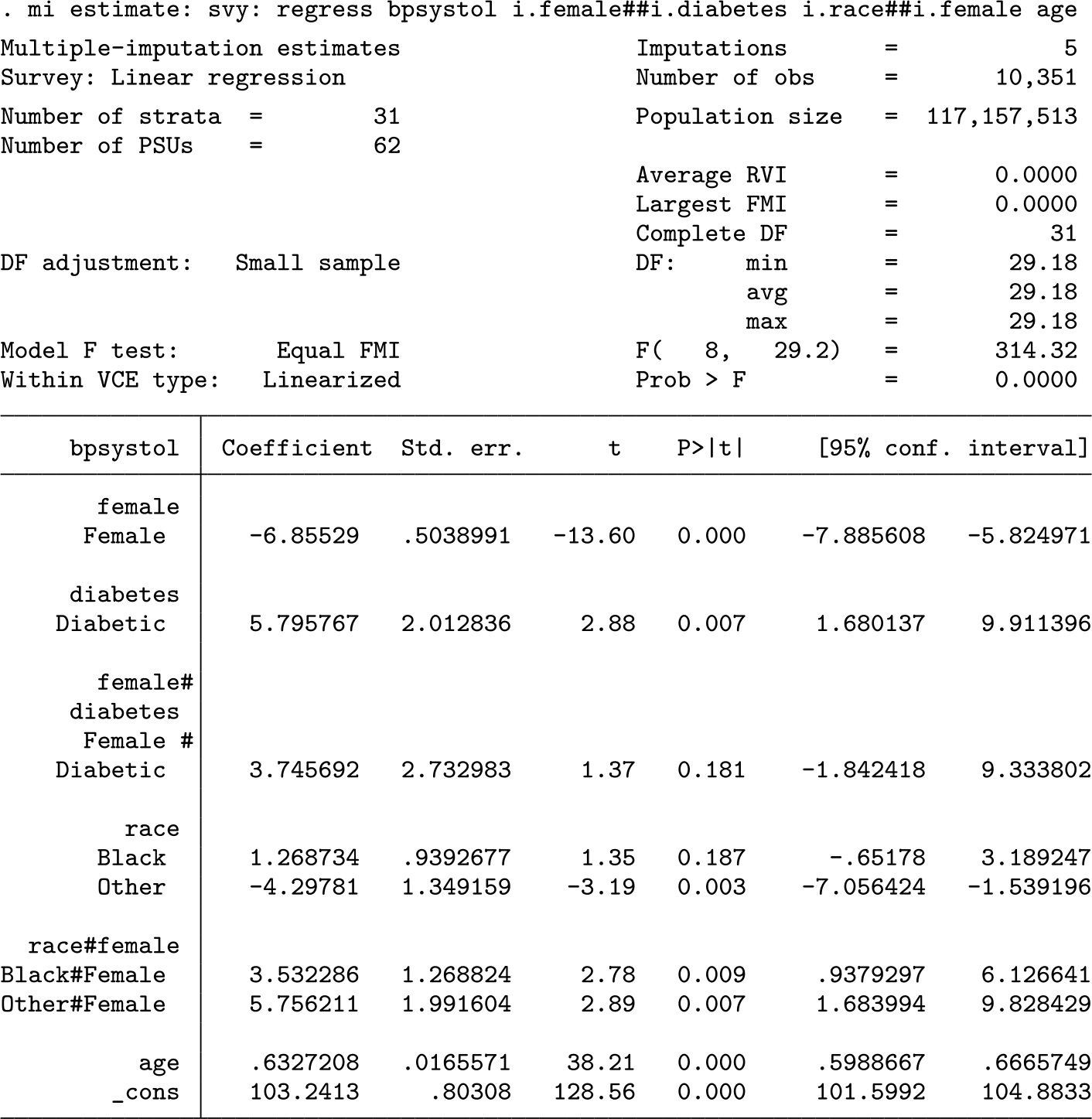
Suppose we are interested in whether systolic blood pressure is higher for females after controlling for BMI, race, and hemoglobin levels. We might specify the following regression model:

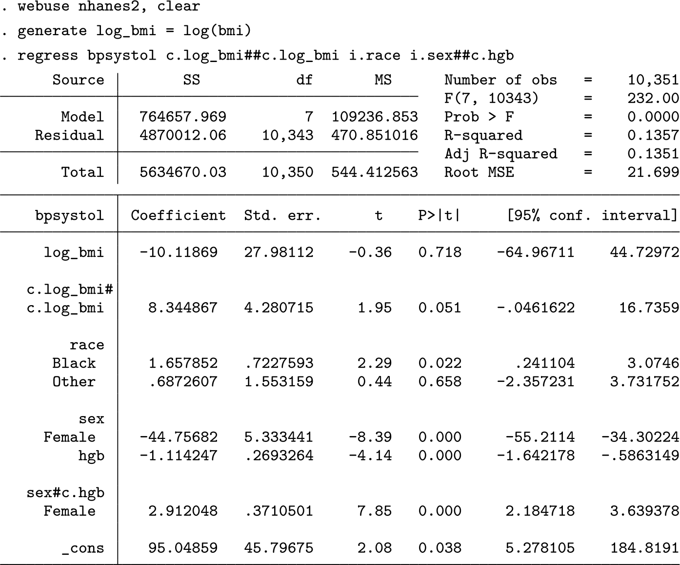
The regression table does not provide a simple answer to the question of whether males or females are predicted to have higher systolic blood pressure. The command margins, pwcompare uses all available information, including all model terms and the proportions of the sample with each distribution of the covariates.

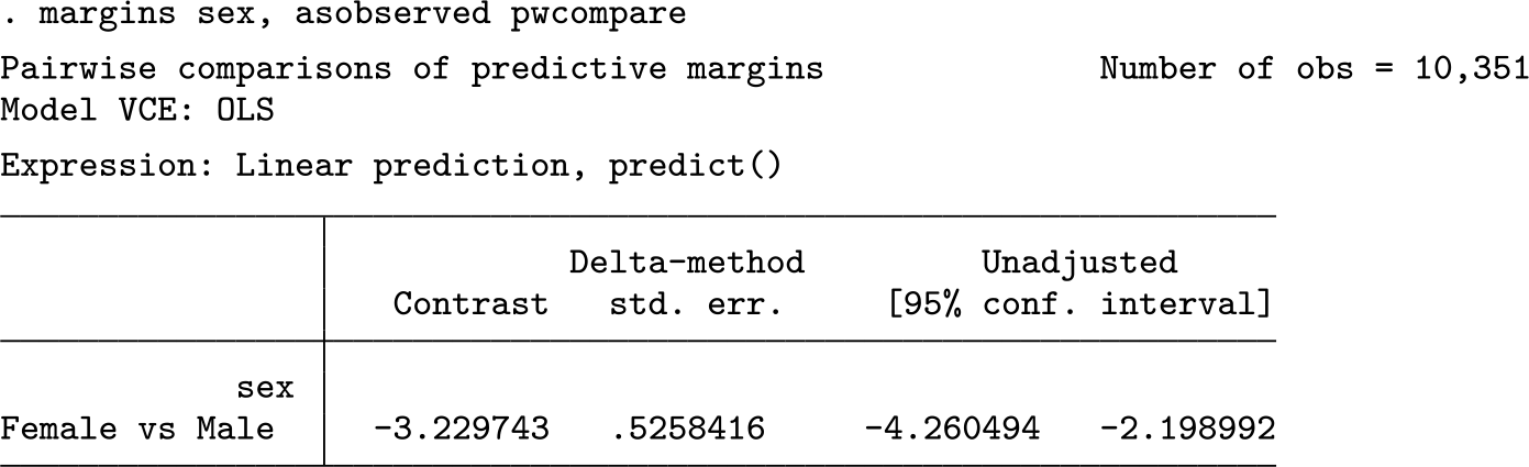
Accounting for all model predictors, margins reports that females in the sample are predicted to have a systolic blood pressure 3.23 points lower than that of males. This difference is clearly statistically significant, but by default margins does not report an effect size, and very small p-values are not an indication of a large effect. It is possible to calculate the effect size by hand using Stata’s base esizei command. First, we need to store the estimated contrast in the scalar we choose to name diff and then use summarize to store the within-group means and standard deviations.

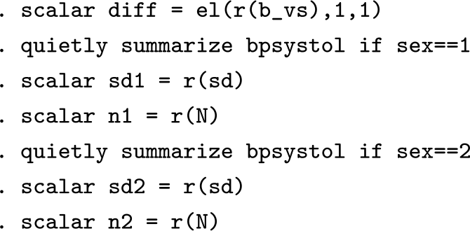
Now that the necessary summary statistics are in memory, esizei will report the effect size for the marginal comparison between males’ and females’ values on the outcome after adjusting for all the predictors in the regression equation, using the values for each group from the margins command. We use the stored coefficient from margins, pwcompare for the first group and a zero for the other.

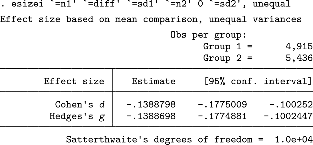
The regression-adjusted difference between males’ and females’ systolic blood pressure is approximately 0.14 standard deviations. Field-specific context informs a judgment about whether this is a large or small difference. Nevertheless, if we are confident in our margins specification, we can be confident in the interpretation of the estimated “d” family effect size.

4.2 Marginal effect sizes for continuous regression predictors

The approach in section 4.1 applies only to dichotomous variables. For continuous predictors, the analyst can report ω ² or η ² statistics or use margins to create a dichotomous comparison. Here we analyze the differences between females with high and low levels of hemoglobin.

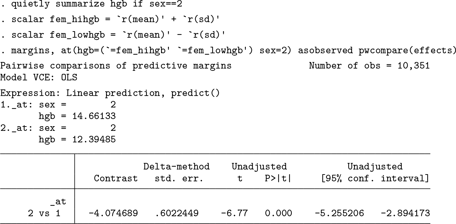
The predicted difference in systolic blood pressure between female subjects with hemoglobin levels 1-standard deviation higher than the mean and 1-standard deviation lower than the mean is 4.07 points. This difference is statistically significant at α = 0.05. Determining practical significance using measures of effect size necessitates figuring the standard deviations. This is complicated by the fact that the approach used to calculate the standard deviation in section 4.1 is not directly available when the predictor in question is continuous. Furthermore, it usually does not make sense to estimate the standard deviation only for cases with a very specific hemoglobin level. For example, in this dataset containing over 10,000 cases, none have a rounded value of hgb that equals the grand mean of 14.3.

There is no single accepted method to define the standard deviations for calculating effect sizes when predictors are continuous. One possibility is to simply use the standard deviation of the outcome variable for both the high and the low values of the continuous predictor (following Cohen et al. 2003). This is analogous to Glass’s Δ approach, so the delta option is specified.

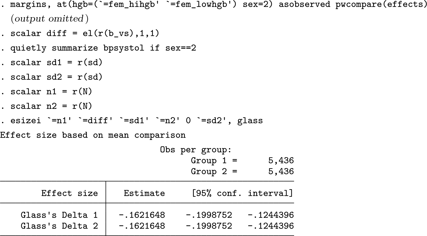
The estimated difference of 0.16 standard deviations helps the analyst understand the magnitude of the effect, which the small p-value does not.

4.3 Marginal effect sizes for recoded continuous regression predictors

There is an even simpler and more straightforward approach to find the denominator: divide cases into a small number of groups based on their value of the continuous predictor, and then substitute the new categorical variable in the regression equation. The advantage of this approach is that there are clearly defined groups for comparison and for calculating the standard deviation. If theory suggests logical thresholds, then Stata’s recode and generate commands are useful for creating the groups. If not, then splitting the variable into quantiles with xtile would also suffice. In this example, there is theoretical guidance for establishing a threshold: hemoglobin levels for men are regarded as elevated when they are above 17 grams per deciliter, while the standard for women is 15 grams per deciliter (Cleveland Clinic 2018). We can create indicator variables for a high hemoglobin level and then reestimate the regression using the indicator variable in place of the continuous measure of hemoglobin. Moving from a continuous measure to a categorical measure results in some loss of efficiency. Still, if a marginal comparison is central to the analysis, the ease of calculating an effect size may justify small reductions in R ² values.

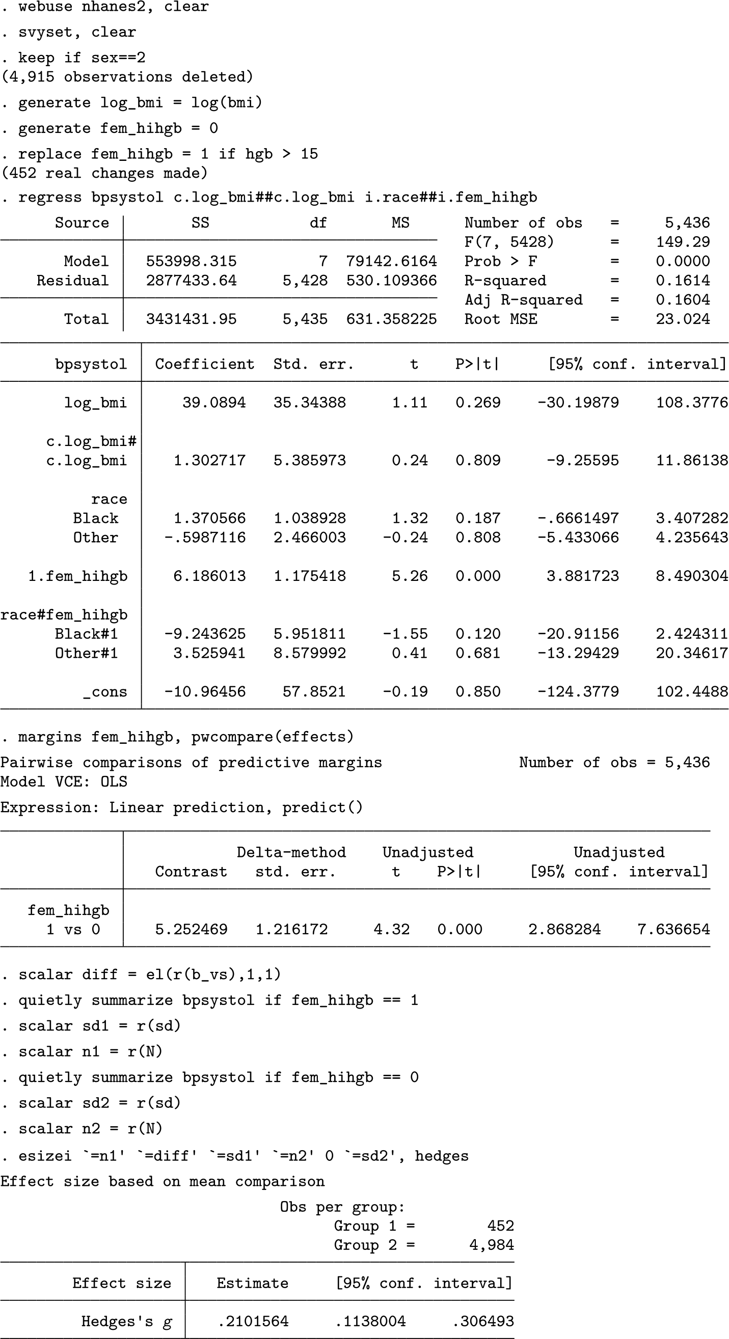
These calculations show that females with clinically elevated hemoglobin levels are predicted to have a systolic blood pressure that is 0.21 standard deviations higher than those without high hemoglobin levels. However, estimating the standardized effect size for a postestimation contrast is cumbersome, particularly with multiply imputed data. Furthermore, esizei does not work with data that are svyset or mi svyset.

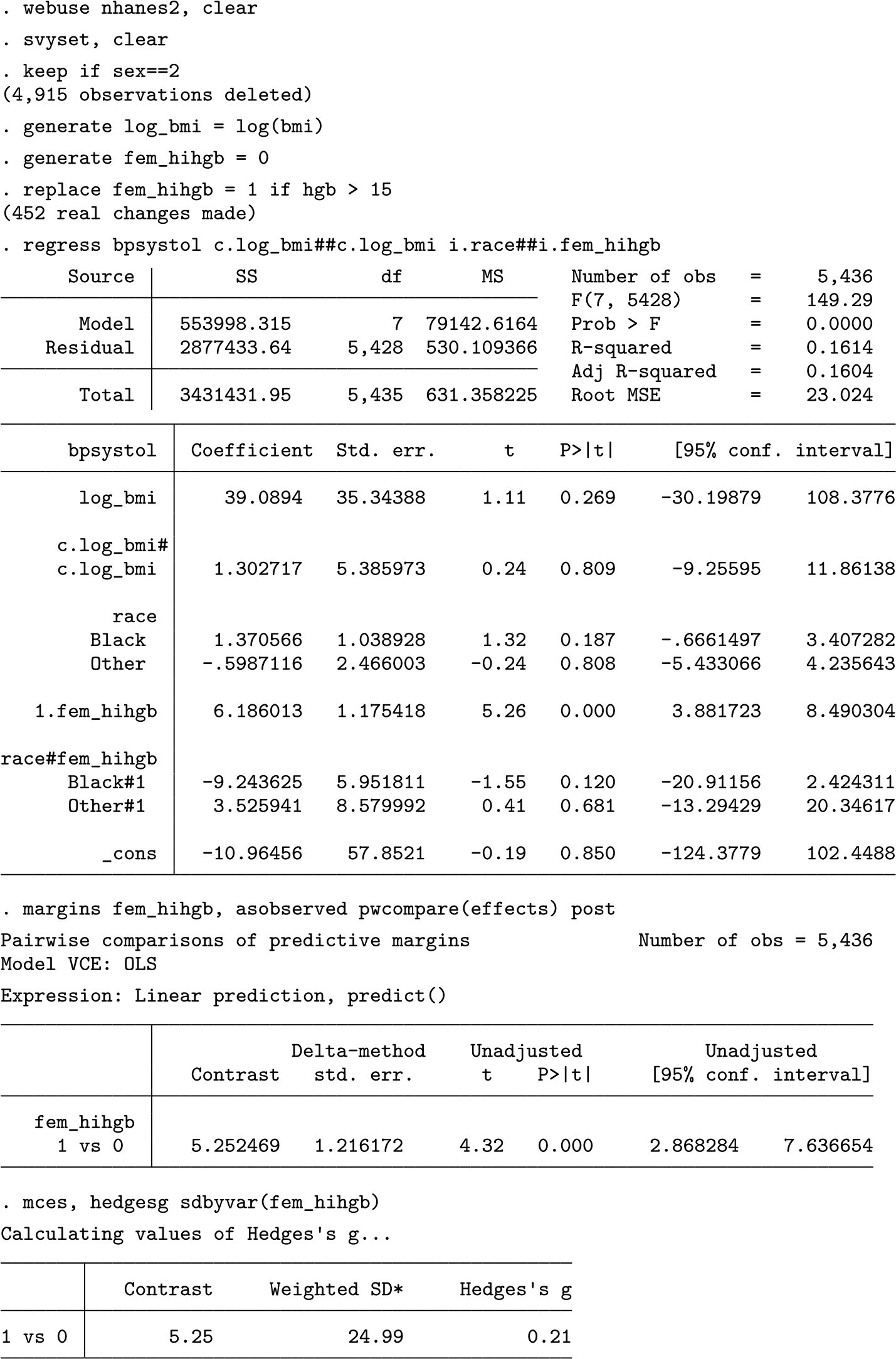
5 The mces and svysd commands

The mces command calculates one of three “d”-family effect-size measures for betweengroup contrasts of marginal effects obtained after margins, pwcompare post. The default effect size, which I am calling the root mean squared error (RMSE)-based Δ, uses the RMSE of the regression as the denominator in a calculation similar to (1)–(3). Hedges’s g and Cohen’s d can be requested as well by specifying a binary grouping variable used to calculate the pooled standard deviations for the same equations. The community-contributed mimrgns command ³ (Klein 2016) for marginal effects with multiply imputed data is also supported, as are complex survey designs specified with svyset or mi svyset.

Alternatively, if an estimate of only the survey-adjusted standard deviation is desired, the svysd command can be used independently of any margins results.

5.1 Syntax

The syntax after margins, pwcompare post or mimrgns, pwcompare post is

mces [, sdbyvar(varname) hedgesg cohensd sdupdate nowarning force ]

The syntax to calculate a survey-adjusted standard deviation only is

svysd depvar, sdbyvar(varname) [unweighted nowarning force ]

The mces command should work with most models based on linear regression that store coefficients from margins, pwcompare post and mimrgns, pwcompare post in the macro e(b_vs), such as regress, truncreg, sem and gsem, and tobit. mces is not appropriate for multilevel models, because it does not account for intraclass correlation (see Lorah [2018]) nor for categorical outcomes or generalized linear models that do not have standard deviations or RMSEs.

A further note about mces is that it estimates the standard deviations based upon all cases in the dataset and not only those used in the estimation. When requesting Hedges’s g or Cohen’s d, users may wish to run keep if e(sample) prior to mces if out-of-sample cases should not be used.

5.2 Options

sdbyvar(varname) specifies a dichotomous variable defining the comparison groups. sdbyvar() is required with svysd.

hedgesg (mces only) requests Hedges’s g instead of the default RMSE-based Δ.

cohensd (mces only) requests Cohen’s d instead of the default RMSE-based Δ.

sdupdate (mces only) requests a recalculation of the standard deviation, which is useful if the dataset has changed since the standard deviation was last calculated.

unweighted (svysd only) requests the unweighted pooled standard deviation used for Cohen’s d instead of the default weighted pooled standard deviation used for Hedges’s g.

nowarning suppresses warning messages about applicability of the standard deviation to the estimated pairwise comparisons.

force bypasses a check of whether the outcome variable is continuous.

5.3 Stored Results

mces and svysd store the following in r():

5.4 Example

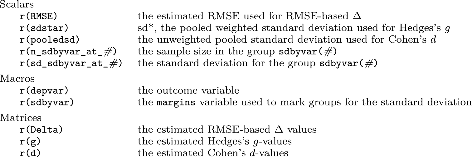
mces can be used to streamline the process outlined in section 4.3. The reported Hedges’s g from mces is equal to the value computed by hand in that example.

The next example demonstrates an application of mces with data that are multiply imputed and have a complex sampling design. The first step is to set up and fit a regression model.

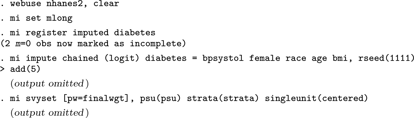
Because the data are mi set, we use the mimrgns command to produce the pairwise comparisons. This example uses a more complex at() statement, which mces supports. By default, the RMSE-based Δ effect size is requested.

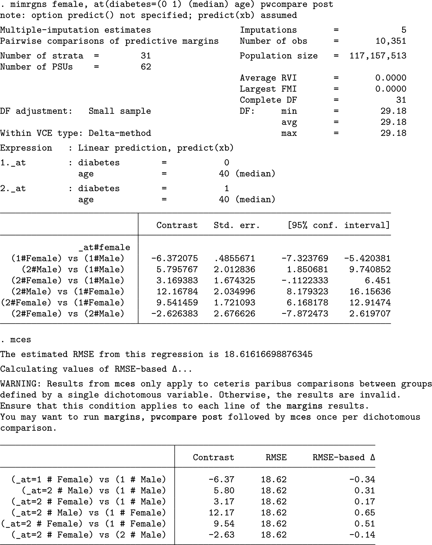
The results include a warning message that warrants explanation. mces does not attempt to second-guess the analysis and uses the estimated RMSE or standard deviation to calculate an effect-size statistic for each line in the margins output. However, margins, pwcompare estimates all possible pairwise comparisons between the variables, regardless of their properties. The analyst must therefore be careful to ensure that the dichotomous grouping variable (the sdbyvar(varname) option, if specified) is the only difference in each comparison. Otherwise, the results are invalid and should not be considered. For a typical six-comparison output from margins, pwcompare with two binary grouping variables (such as one at() and one over()), the first and last lines will be the only two that meet these conditions. For clarity and to avoid errors, separate margins or mimrgns statements can be used to formally specify the desired comparison.

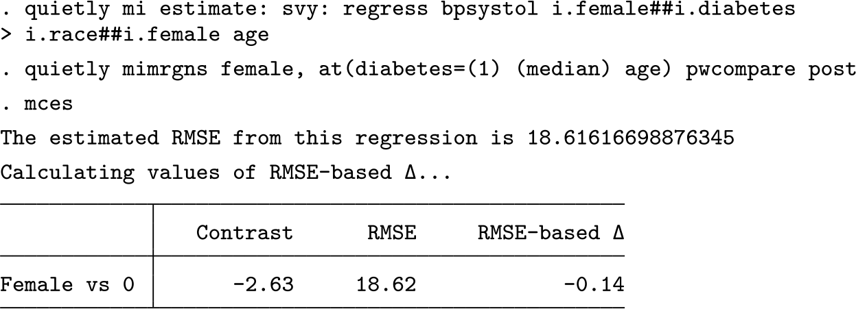
Because the post option in the margins, pwcompare command has cleared the stored regression results, the model needs to be refit for additional comparisons using mces. estimates store can help to save run time if the model is computationally intensive.

6 Conclusion

Both regression-based modeling and standardized effect-size measures are increasingly prevalent in applied quantitative research, yet existing effect sizes for complex regression models have been unsatisfying. mces offers an additional avenue for estimating effect sizes with linear models.

Because mces‘s functionality is limited to models with continuous outcomes, this is an area that offers possible avenues for future development. Applications to additional types of models, such as generalized linear models, multilevel models, and longitudinal models, would extend researchers’ abilities to report standardized effect sizes to further complement or replace null hypothesis significance testing in more contexts.

8 Programs and supplemental materials

Supplemental Material, sj-zip-1-stj-10.1177_1536867X221083901 - Effect sizes for contrasts of estimated marginal effects

Supplemental Material, sj-zip-1-stj-10.1177_1536867X221083901 for Effect sizes for contrasts of estimated marginal effects by Brian P. Shaw in The Stata Journal