
Abstract
Self-reported survey data are often plagued by the presence of heaping. Accounting for this measurement error is crucial for the identification and consistent estimation of the underlying model (parameters) from such data. In this article, we introduce two commands. The first command,
Keywords
1 Introduction
A problem frequently encountered in survey data is the abnormal concentration of reported observations at certain values of the outcome variable. Examples include reported dates of death in neonatal mortality data (Arulampalam, Corradi, and Gutknecht 2017, ACG from now on), age of starting and quitting cigarette smoking (Forster and Jones 2001), or self-reported consumption expenditure data (Pudney 2008). One of the main reasons for such concentration, often referred to as heap points, is rounding. Correctly identifying and accounting for the rounding behavior is crucial for consistent estimation of and valid inference on the parameters of the underlying model of interest. ACG discusses identification and estimation of popular duration and ordered choice models, in the presence of heaping, using maximum likelihood procedures.
In this article, we introduce the command
As shown in ACG, when some of the parameters lie on the boundary of the parameter space, the limiting distribution of the estimator is no longer a normal distribution, and more complicated subsampling procedures are required for inference. Hence, we also provide two specification tests. The first one tests for the absence of heaping effects in the model. The second specification test examines whether all heaping parameters lie inside the parameter space, which in turn will allow for inference based on asymptotic normality. We use the so-called M out of N bootstrap method to calculate the standard errors. These tests provide a set of tools that enable applied researchers to verify the validity of different model specifications.
In appendix A, we show how the
2 MPH model with “heaping”
2.1 Specification
We start with the MPH model for the unobserved true durations in continuous time and parameterize this for individual i as

where λ
0(τ
∗) is the baseline hazard at time τ
∗, ui
is the individual unobserved heterogeneity (frailty), and
where
More specifically, the form of misreporting we address is referred to as “heaping” in the literature and describes the phenomenon of observing an over- and underreporting of failures at certain time periods. We briefly list informally the set of assumptions for the derivation of the estimator and its properties here and refer the readers to ACG for further details on the assumptions and identification results. 1 Based on the neonatal mortality illustration from ACG, we also illustrate our command using a simulated dataset based on ACG.
Assumptions
A1 Excessive concentrations of reported failures occur at time periods that are multiples of a positive integer. This implies equal distance between the heap points. In most of the empirical applications where we see heaping because of rounding, we often see the distance between heaping points to be the same. This is the scenario
A2 To identify the baseline hazard from possibly misreported observations, we need to impose a structure on the heaping process. In the illustration provided here, we assume that one period to the right and to the left of each heap point are associated with that heap. We denote the maximum number of time periods that a duration can be rounded to as
A3 All heaping is to observed duration points only. In our example, this implies that the heaping is to the points 5, 10, and 15 only, because we assume that the outcome variable is censored at 18 days. The maximum number of heaps is assumed to be
A4 The censoring is exogenous, and the censored observations are correctly reported.
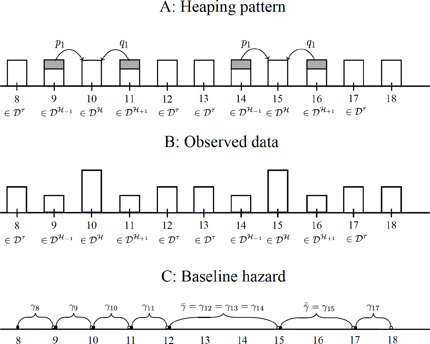
A5 Whenever the true duration falls onto one of the heaping points, it will be correctly reported. However, whenever the duration falls onto the nonheaping points, it is assumed to be either correctly reported or rounded (up or down) to the nearest heaping point. Let p 1, p 2, etc., denote the corresponding rounding up probabilities when a true duration is lower by one, two, etc., units from the nearest heaping point. Similarly, let q 1, q 2, etc., denote the rounding down probabilities when a true duration is higher by one, two, etc., units from the nearest heaping point. In our illustration, a reported duration of, say, 10 days includes true durations of 11 (9) days, which have been rounded down (up) to 10 days (see figure 1). Hence, p 1 is the probability that a true duration of 9 will be rounded up to 10 days. Analogously, q 1 is the probability that a true duration of 11 will be rounded down to 10 days..
Stylized example
A6 There exists a segment in the baseline hazard that is constant from time period
Heuristically, the assumption that the hazard is constant over a set of time periods, which includes (at least) a known true value, enables us to uniquely identify the γ parameter associated with this correctly reported time period as well as the parameters of the heaping process, that is, the ps and the qs, in this region, from the observed data. Subsequently, we can use these identified probability parameters to pin down the rest of the baseline and other hazard parameters. See figure 1.
2.2 Maximum likelihood estimation
Before writing down our likelihood function, we first define some notation.
Let
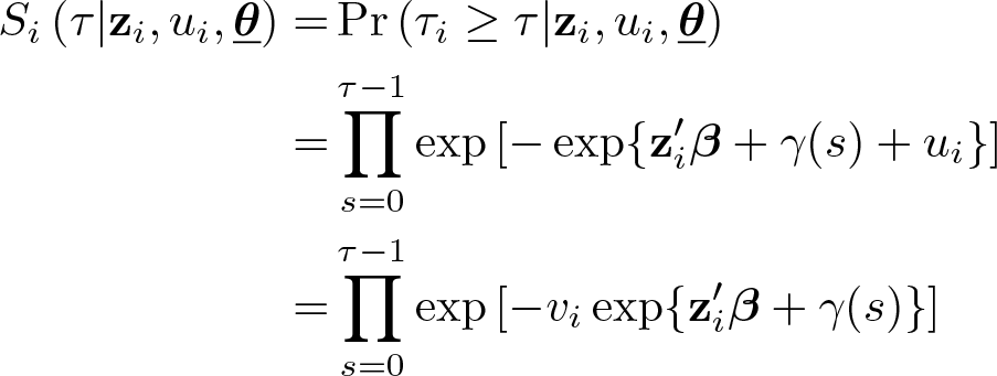
where vi ≡ exp(ui ) and ui is the unobserved heterogeneity.
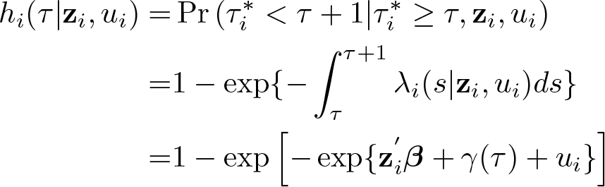
The probability for an exit event in τi <
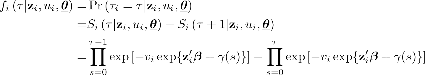
fi
(τ|
Henceforth, let

with ti denoting the discrete-reported duration.
The likelihood contributions depend on the following four cases: For correctly reported durations, ϕi
(t|
For reported durations that are l = 1, 2, etc., points below the nearest heaping point, ϕi
(t|
Similar to (II), for reported durations that are l = 1, 2, etc., points above the nearest heaping point, ϕi
(t|
Finally, for reported durations on the heaping points,

In summary, there are four different probabilities of exit events depending on the nature of the true duration.
We next write down the corresponding unconditional probabilities under a set of assumptions on the unobserved heterogeneity vi
. More specifically, we impose the following assumptions on the properties and the distributional form of vi
, which are standard in the duration literature:
vi
is identically and independently distributed over i and is also independent of
vi
follows a Gamma distribution with unit mean and variance σ.
3
The unconditional probabilities under the above assumptions, in case (I) above are given by
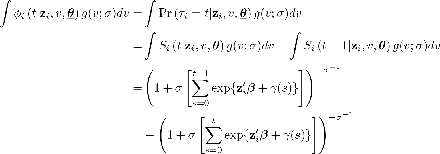
where the last equality uses the fact that there is a closed-form expression under the Gamma density assumption for v (for example, see Meyer [1990, 770]). Moreover, because the integral is a linear operator, the probabilities for the cases (II) to (IV) can be derived accordingly.
Our next goal is to obtain consistent estimators for
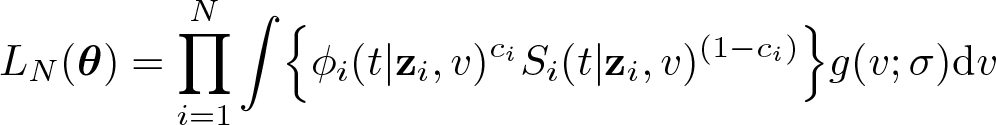
Let ci be an indicator equal to one if the observation is uncensored and zero otherwise. It is assumed that durations are censored at a fixed time τ that exceeds the points that are rounded and is not one of the heaping points. Assuming that censoring is independent of the heaping process and the durations, we have the following unconditional likelihood contributions. 4
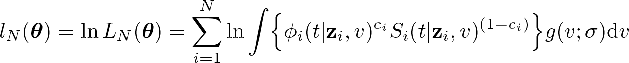
The likelihood function for the observed sample is
and so
Given the definition of ϕi
(t|
Under the assumptions provided in ACG, we see that the limiting distribution of the estimator depends on whether some heaping probability parameters lie on the boundary of the parameter space, that is, whether one or more of the “true” probability parameters are equal to zero. In this case, the limiting distribution is no longer normal because the information matrix is not block diagonal in general but takes a different form. We use the M out of N bootstrap method to derive the asymptotic standard errors. Details are provided in ACG.
3 Ordered probit model with heaping: Specification and estimation
In general, there are many observed discrete outcomes (other than durations) that can exhibit heaping. For instance, survey data on the number of doctor visits or on cigarette consumption in a given period of time is often subject to this phenomenon. Here we discuss the estimation of an ordered probit model allowing for heaping. In appendix C, we provide a discussion on the link between the discrete duration model derived from the PH specification and the ordered choice model. To keep notational clutter to a minimum, we do not explicitly show the conditioning set in what follows.
Consider the following latent-variable model representation of an ordered choice model, 5
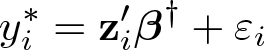
where

where κ
0,…, κJ
are the threshold parameters that divide the real line into a finite number of intervals. Here we have assumed the normalizations κ
0 = −∞, κJ
+1 = +∞, and κj < κj
+1. In addition, note that we require a scale normalization, so
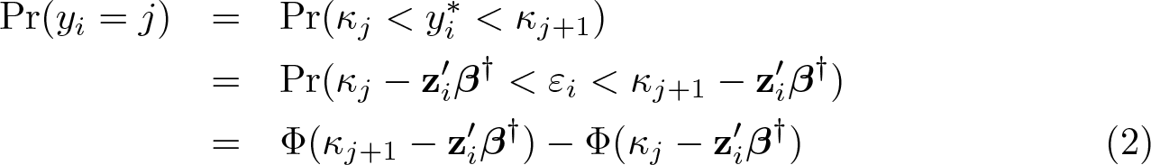
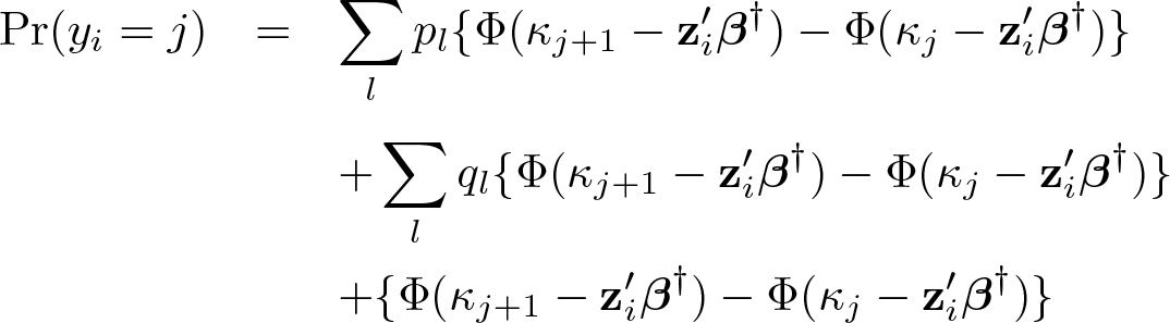
In the presence of heaping data, the term Pr(yi
= j) depends on the four cases: For correctly reported outcomes, For reported outcomes that are l = 1, 2, etc., points below the nearest heaping point, Similar to (II), for reported outcomes that are l = 1, 2, etc., points above the nearest heaping point, Finally, for reported outcomes on the heaping points,
Note that when the outcome is duration data and for right-censored data at yi
=
the likelihood function can be written as
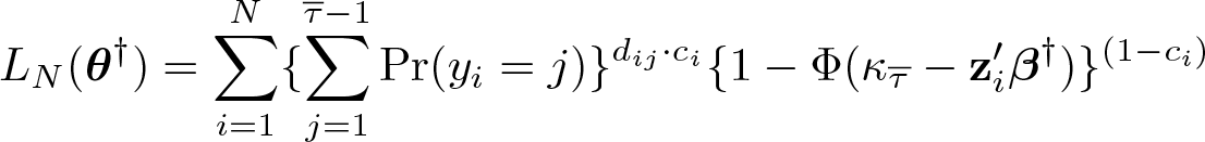
where
4 Testing for “heaping”
As pointed out in section 2.2, if some of the heaping probability parameters lie on the boundary of the parameter space, the asymptotic distribution of the estimator is no longer normal. In addition, inference becomes more complicated, because subsampling methods are used to derive the asymptotic standard errors. In the following, we discuss two specification tests: first, a test to detect whether heaping matters in a statistical sense
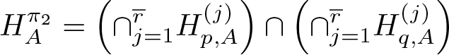
Thus, collecting all heaping parameters in the vector

versus

for some l = 1,…,
The second specification test examines whether all heaping parameters lie inside the parameter space, which in turn allows inference based on asymptotic normality. That is, the null hypothesis of the test is that at least one rounding parameter is equal to zero versus the alternative that none is zero (and thus no boundary problem exists). Therefore, if we reject this hypothesis, we can make inference based on standard normal critical values, while if we fail to reject, we ought to rely on subsampling methods for inference.
Formally, let
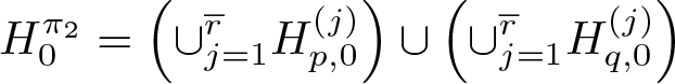
versus
so that under
We now introduce a rule to discriminate between
Thus, as pointed out above, if one rejects
5 Command implementation
As discussed in the earlier section, if one or more of the probability parameters lie on the boundary of the parameter space, the asymptotic distribution of the estimator is no
longer normal. We provide two tests that can be used to detect this. Hence, the output provides the usual asymptotic standard errors along with the standard errors calculated using the M out of N bootstrap method, where M denotes an integer strictly smaller than N (see ACG).
5.1 Data
We illustrate the use of the
The latent dependent variable

We use two different schemes to generate εi
for demonstrating For the For the data example used to demonstrate
Note that we keep the function flat from period 12 to 15. The discrete duration variable without heaping, for each observation i = 1, 2,…, 250, for these models is then generated using the cutoff points as

where we assume δ 0 = −∞ and δ 19 = ∞ for the normalization.
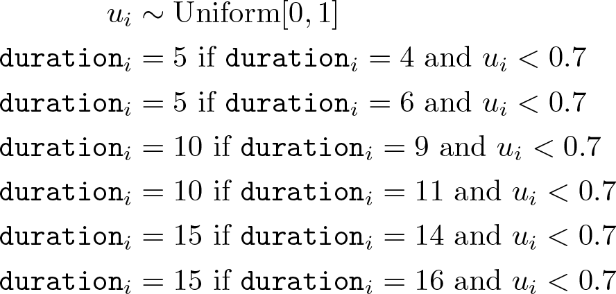
Finally, we add the following heaping pattern to the dependent variable: the duration points 4, 9, and 11 are rounded up to 5, 10, and 15, respectively, with probability 0.7, and the duration points 6, 11, and 16 are rounded down to 5, 10, and 15, respectively, with the same probability, 0.7. Hence, the heaping probability parameters are p
1 = q
1 = 0.7. Algebraically, the actual observed duration variable
We have not included the unobserved heterogeneity in the generation of the above data. Figure 2 plots the histograms of both the observed duration variable with heaping and the true duration variable without heaping as generated from the ordered probit model.
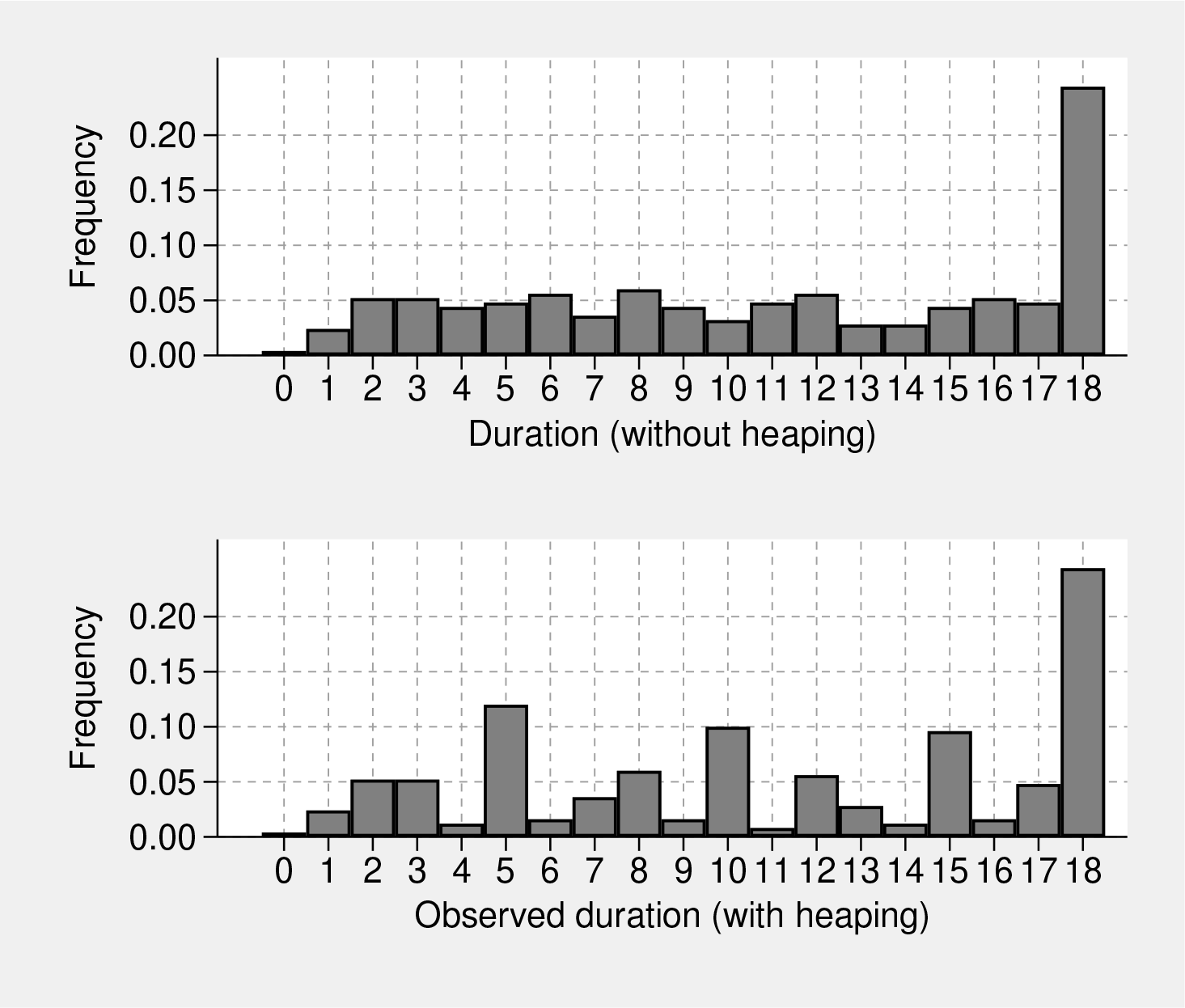
Histograms of the duration variable in the example data for demonstrating the
5.2 The heapmph command
This section describes the implementation of the
Basic syntax
The basic syntax of the
where depvar stands for the dependent variable and varlist may contain the specified covariates. In this article, we demonstrate the usages of the
Model estimation
As discussed in section 5.1, the analysis is restricted to modeling the hazard rate during the first 18 days after birth because the reported number of deaths is smaller after this period (see ACG). We therefore add the
We next detail the values used for the four compulsory options to define the pattern of heaping in our example. Because we have generated the data with heaps at days 5, 10, and 15, we define the starting period (h
∗) of 5 using the option We set option As illustrated in our stylized example (figure 1), the rounding probabilities are p
1 and q1, respectively. Hence, with the number of heaping probabilities, we have the maximum number of time periods that a duration can be rounded to denoted as The constant part of the baseline hazard enables us to identify the parameters of the heaping process. In this example, we set the time period after which the hazard is constant equal to 12 (
Example
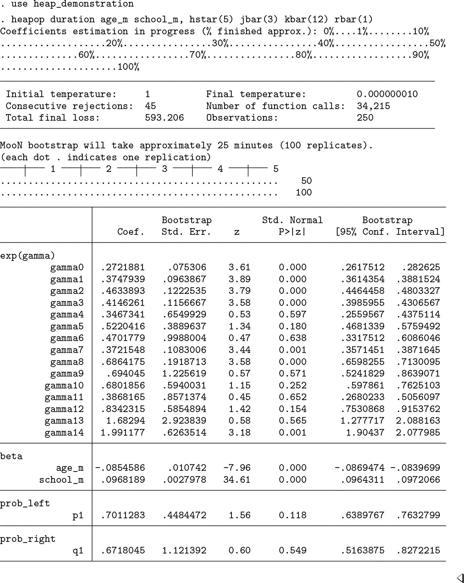
We choose

The command first employs a single simulated annealing SA algorithm (see section 5.5.3 of ACG) to solve for the point estimates. The M out of N bootstrap procedure is then conducted to yield the standard errors. Note also that the 95% bootstrap confidence interval is constructed using the 2.5% and the 97.5% quantile of the empirical bootstrap distribution. The output table consists of five panels. The panel
Panel
Testing for the presence of heaping effects
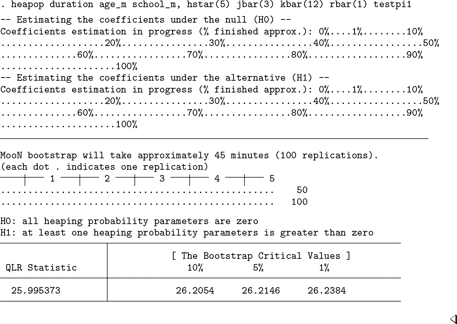
This command provides a subroutine to test null hypothesis via the LR test described in remark 4.2 in section 4 of ACG and briefly discussed in section 4 in this article. We provide a test that can be implemented by adding an option (
Example
To test for the presence of heaping effects under the model specification described in the last subsection, we can simply add the
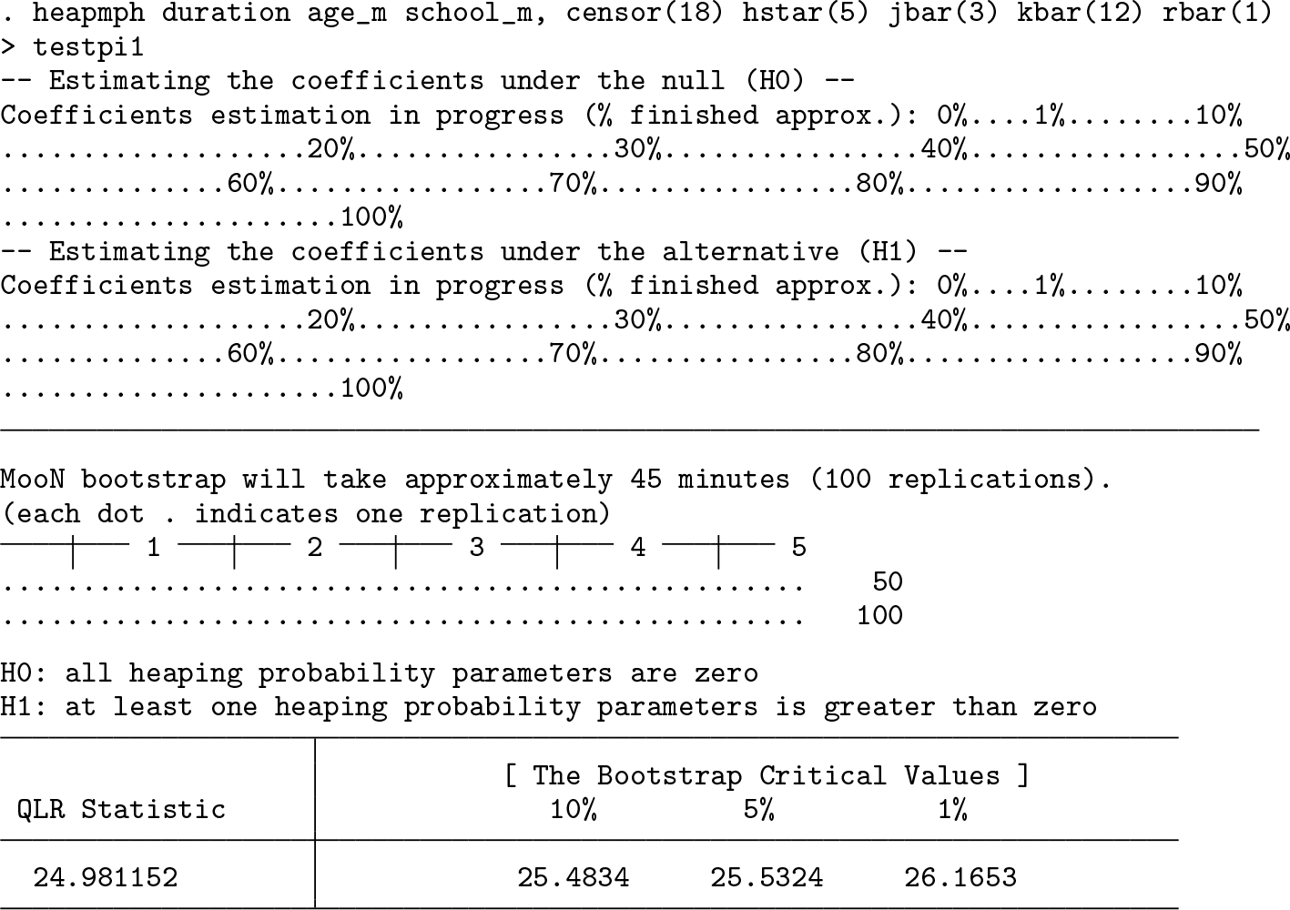
The output table reports the test statistic along with the corresponding bootstrapped critical values at 10%, 5%, and 1% levels. 12 In this example, we fail to reject the null hypothesis at the 10% significance level, which suggests that there is no clear evidence of heaping.
In addition, we employ the IUP rule to test the null that at least one heaping probability parameter is equal to zero
5.3 The heapop command for the ordered probit model with heaping
Basic syntax
The syntax and corresponding options of command
Model estimation
The
This section attaches example usages of the
We first request Stata implement the
Example
Unlike the table in section 5.2, this table consists of only four panels because no unobserved heterogeneity parameter has been estimated. Standard errors and bootstrap confidence intervals are constructed as before in section 5.2. The first panel contains again the estimated baseline parameters (
Testing for the presence of heaping effects
Example
To test for the presence of heaping effects
As in the previous section, we cannot reject the null
5.4 Further options
Here we elaborate on a few additional options, which are available for both commands
Bootstrap options
The
When choosing the M in the M out of N bootstrap, users can set the option
Optimization
The provided commands implement the SA algorithm to maximize the likelihood function of the model. The SA method, proposed by Kirkpatrick, Gelatt, and Vecchi (1983), is a popular local search algorithm for stochastically approximating the global optimum of a given objective function. The review of the algorithm and its technical details can be found in Dowsland and Thompson (2012), for example. The SA algorithm is particularly useful for our model and may be preferable to the conventional Newton algorithm, because SA is better at locating global maximum when the likelihood function is complex, as in our case.
The
Display options
For diagnosing and monitoring purposes, we provide the following two options to display the intermediate command outputs. First the
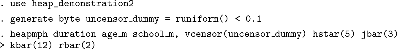
Different censoring points for each observation
The option for variable censoring is
Let
Note that if neither
6 Conclusion
Discrete-time duration models are very popular among researchers. The command
8 Programs and supplemental materials
Supplemental Material, st0603 - heap: A command for fitting discrete outcome variable models in the presence of heaping at known points
Supplemental Material, st0603 for heap: A command for fitting discrete outcome variable models in the presence of heaping at known points by Zizhong Yan, Wiji Arulampalam, Valentina Corradi and Daniel Gutknecht in The Stata Journal
Footnotes
7 Acknowledgments
We are grateful to the British Academy (grant number: SG160731 - Estimation and inference with heaped data - a novel approach), for funding this project. Zizhong Yan acknowledges the support from the 111 project of China (project number B18026). We also thank David M. Drukker and a referee for helpful comments and discussions.
8 Programs and supplemental materials
To install a snapshot of the corresponding software files as they existed at the time of publication of this article, type
Notes
References
Supplementary Material
Please find the following supplemental material available below.
For Open Access articles published under a Creative Commons License, all supplemental material carries the same license as the article it is associated with.
For non-Open Access articles published, all supplemental material carries a non-exclusive license, and permission requests for re-use of supplemental material or any part of supplemental material shall be sent directly to the copyright owner as specified in the copyright notice associated with the article.