A new cure model accounting for longitudinal data and flexible patterns of hazard ratios over time

Abstract

With the advancement of medical treatments, many historically incurable diseases have become curable. An accurate estimation of the cure rates is of great interest. When there are no clear biomarker indicators for cure, the estimation of cure rate is intertwined with and influenced by the specification of hazard functions for uncured patients. Consequently, the commonly used proportional hazards (PH) assumption, when violated, may lead to biased cure rate estimation. Meanwhile, longitudinal biomarker measurements for individual patients are usually available. To accommodate non-PH functions and incorporate individual longitudinal biomarker trajectories, we propose a new joint model for cure, survival, and longitudinal data, with hazard ratios between different covariate subgroups flexibly varying over time. The proposed joint model has individual random effects shared between its longitudinal and cure-survival submodels. The regression parameters are estimated by maximization of the non-parametric likelihood via the Monte Carlo expectation-maximization algorithm. The standard error estimation applies a jackknife resampling method. In simulation studies, we consider crossing and non-crossing survival curves, and the proposed model provides unbiased estimates for the cure rates. Our proposed joint cure model is illustrated via a study of chronic myeloid leukemia.

1. Introduction

In clinical studies, longitudinal biomarkers are usually available to track patients’ disease progression and evaluate treatment effects on survival. One may attempt to analyze longitudinal and time-to-event data separately. However, there are limitations on this simple approach. One of the concerns is the potential presence of informative censoring when the correlations between longitudinal and survival data are not taken into account. Consequently, joint modeling of longitudinal and survival data is more commonly accepted. Moreover, when they are jointly modeled, more precise parameter estimation and more efficient statistical inference would be obtained. ¹ Most joint models incorporate individual-level random effects that are shared between and impact both the longitudinal and survival submodels. Papageorgiou et al. ² presented an overview of joint modeling, and Ibrahim et al. ³ discussed advantages of joint models for longitudinal and survival data in cancer clinical trials. Furthermore, joint models have the ability to predict patients’ risks at an individual level.

A proportion of patients with some diseases may be cured after treatment and thus never experience the failure event of interest (e.g., disease recurrence); such diseases include but are not limited to colorectal cancer,^4–6 leukemia, ⁷ and breast cancer.^8,9 Their survival time distribution (cured and uncured combined), when estimated by the Kaplan–Meier (KM) method, presents a stable plateau at its right tail, given a sufficiently long follow-up time. Various cure models are proposed to model survival data with a cure fraction.

The two main groups of cure models are the mixture cure model and the promotion time cure (PTC) model, introduced by Boag ¹⁰ and Yakovlev and Tsodikov, ¹¹ respectively. Amico and Keilegom ¹² and Peng and Yu ¹³ provided a comprehensive summary of cure models. The mixture cure models could be parametric,^10,14–16 semi-parametric,^17–20 or non-parametric.^21,22 Milienos ²³ introduced a new reparameterization of a flexible family of cure models including the mixture cure model incorporating data with a small or no cured proportion. Safari et al. ²⁴ proposed an estimation method for the latency function (of the susceptible patients) in the mixture cure model when the cure status is partially available. In the mixture cure model for the interval-censored data, Pal et al. ²⁵ implemented the support vector machine approach to estimate the cure proportion, and Pan et al. ²⁶ proposed a Bayesian estimation method.

Different forms of the PTC model have been proposed, such as the proportional hazards cure (PHC) model,^27,28 a parametric cure model, ²⁹ and a non-parametric PTC model. ³⁰ Liu and Shen ³¹ developed a PTC model for the interval-censored data. Pal and Aselisewine ³² proposed to use a support vector machine method to model the incidence part of the PTC model. However, only a limited number of studies focused on cure models’ performance when some covariates violate the proportional hazards (PH) assumption. Unlike the traditional cure models, some models utilize frailty terms to explain observed and unobserved heterogeneity among patients.^33–36 Although these proposed models allow for covariates’ non-PH structures, they bring additional assumptions on survival data and contain complex model structures.

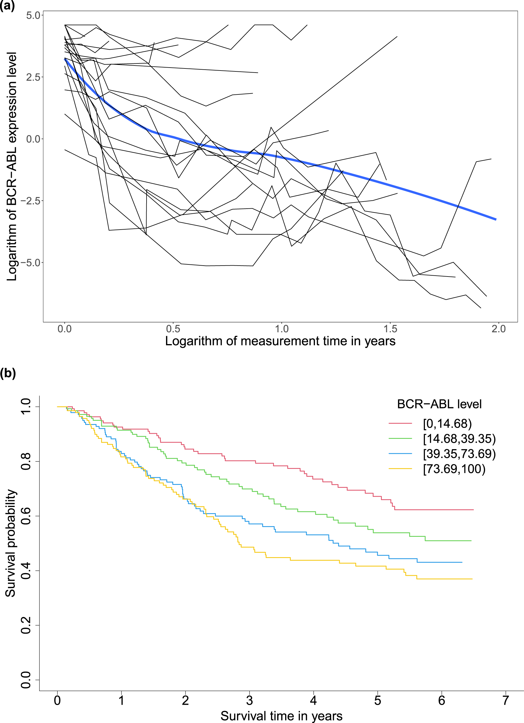
A motivating example for our study is a randomized phase III study (CA180-034) for dose optimization. ³⁷ It compared different dose schedules of dasatinib in 670 patients with chronic-phase chronic myeloid leukemia (CML) who could not receive imatinib anymore due to resistance or intolerance. CML is caused by an error of a chromosomal translocation, occurring on the Abelson (ABL1) protooncogene in chromosome 9 and the breakpoint cluster region (BCR) gene in chromosome 22.^38,39 In this data set, the BCR-ABL fusion gene’s expression level was a longitudinal biomarker varying between 0.03 and 99.99, reflecting how well dasatinib inhibited the growth of the BCR-ABL expressing gene for each patient within the time of the study. ⁴⁰ The event of interest was disease progression. All patients’ times to progression statuses were recorded as survival outcomes. Among all patients, 566 patients had at least one longitudinal value during the follow-up time. Figure 1(a) presents the trajectories of randomly selected 20 patients’ logarithms of BCR-ABL expression gene levels as the black curves and the overall trajectory of all 566 patients’ logarithms of BCR-ABL expression gene levels as the blue curve over the logarithms of the measurement times in years smoothed by the loess function. With the treatment, patients tended to have less severe disease status on average over time reflected by the decreasing overall curve. Figure 1(b) shows KM estimates of progression-free survival (PFS) by groups of baseline BCR-ABL expression levels categorized by the quartiles. The stable plateau at the right tail of each survival curve indicates a proportion of cured patients in the corresponding subgroup. The non-parametric test of Maller and Zhou ⁴¹ further verified the existence of the cure proportions in all the baseline BCR-ABL expression level groups and among all patients ( $p$ -values $<0.01$ ). Patients with lower baseline BCR-ABL expression levels tended to have larger short- and long-term survival probabilities.

Figure 1.

(a) Trajectories (black curves) of randomly selected 20 patients’ and the overall trajectory (blue curve) of 566 patients’ logarithms of BCR-ABL expression gene levels over logarithms of measurement times and (b) Kaplan–Meier estimates of progression-free survival by groups of baseline BCR-ABL expression levels defined by the quartiles (14.68, 39.35, and 73.69) in the chronic myeloid leukemia study for 566 patients with at least one follow-up biomarker measurement after the baseline. BCR: breakpoint cluster region; ABL: Abelson.

In this motivating example, to obtain patient subgroups’ cure rates, we can use the baseline information only, which may result in biased estimated cure rates. Therefore, we must jointly model longitudinal and cure-survival data to incorporate the correlation between longitudinal and survival data and the within-patient correlation of repeatedly measured biomarker values. In the joint modeling framework, we encounter a baseline covariate’s violation of the PH assumption. In detail, the baseline predictors that we are most interested in are the dose level (100 or 140 mg daily) and age (< or $\ge 60$ years). The Grambsch-Therneau test ⁴² revealed that only the age group did not follow the PH assumption (p-value = 0.026) in a Cox PH model with the following covariates: dose level group, age group, and baseline BCR-ABL expressing gene levels. Therefore, we need to have a cure submodel that can handle covariates’ non-PH structure in the joint model. This motivating example demonstrates the need for cure models that can deal with the violation of the PH assumption while jointly modeling the longitudinal and cure-survival data to improve cure rate estimation for patient subgroups.

Several approaches have been proposed for the joint modeling of longitudinal and cure-survival data. The joint model proposed by Law et al. ⁴³ modeled the longitudinal biomarker by a nonlinear hierarchical mixed-effects submodel and the time-to-event data by a time-dependent Cox PH submodel conditional on random effects. Yu et al.^44,45 also implemented a nonlinear hierarchical mixed submodel to model the longitudinal data, but the cure-survival data was modeled by a mixture cure submodel with a time-dependent PH model for susceptible patients and a logistic function for the cure fraction. Pan et al. ⁴⁶ proposed a joint model with the longitudinal data modeled by a linear mixed (LM) submodel and the cure-survival data modeled by a mixture cure submodel, and the properly scaled random effects connect these two submodels. The joint model proposed by Yang et al. ⁴⁷ modeled longitudinal measurements by implementing a partly LM submodel with the $B$ -spline and fit a semi-parametric mixture cure submodel with shared gamma frailty and baseline hazard formed with $B$ -spline for survival data with a cure fraction. Barbieri and Legrand ⁴⁸ applied mixture cure submodels for time-to-event outcomes with cures, but they focused on different latent structures linking the mixture cure submodel and the LM submodel. Ekong et al. ⁴⁹ proposed a joint model with longitudinal outcome modeled using spline function and survival outcome modeled by the PH mixture cure model, where the two models were connected by shared random effects. The proposed joint model was estimated by approximate Bayesian inference using latent Gaussian models.

There are also a few joint models using the PTC submodel for cure-survival data. In the work of Brown and Ibrahim, ⁵⁰ the joint cure-rate model was formulated by modeling the longitudinal measure from a mixture distribution with a point mass at zero and adding time-vary covariates into the PTC submodel. Song et al. ⁵¹ used the random effects from a LM submodel to link the longitudinal and PTC submodels. Kim et al. ⁵² had a non-parametric baseline distribution $F_0(t)$ in the PTC submodel and integrated the PH and odds cure models into a general form. Chi et al. ⁵³ proposed a joint cure model for longitudinal ordinal categorical item response data, whose cure submodel was a PTC model with the PH assumption. A few studies have considered longitudinal and cure-survival data with multiple longitudinal biomarkers.^54,55 These joint cure models have not been assessed to have the ability to handle the violation of the PH assumption.

Even though a few studies have incorporated the longitudinal data into the cure models, to the best of our knowledge, no existing cure model has considered longitudinal biomarkers and also emphasized or evaluated the performance under the situation when some covariates follow the PH assumption while others do not. A false PH assumption can lead to biased cure rate estimates for patient subgroups, which may convey misleading messages about patients’ disease status or the effect of clinical treatments. We propose a new model accounting for longitudinal data and flexible patterns of hazard functions to simultaneously handle some baseline covariates with the PH structure and others with the non-PH structure in the longitudinal and cure-survival data.

In our joint model, we extend the PHC model to relax the PH assumption via flexible patterns of hazard functions for the cure-survival data and employ an LM-effects submodel for the longitudinal biomarker. The two submodels from the joint model share a common set of patients’ random effects. The cure submodel is named a flexible-hazards cure (FHC) submodel. Due to the flexible hazard functions, the FHC submodel does not force constant hazard ratios for different covariate levels of the baseline covariates over time. We implement a non-parametric maximum likelihood estimation method incorporating the Monte Carlo expectation-maximization (MCEM) algorithm for parameter estimation. In the FHC submodel, the standardized baseline cumulative hazard function $F_0(t)$ has a non-parametric form and is estimated by the Lagrange multiplier method. The standard error estimation is achieved by the jackknife resampling method. In summary, compared to the existing models, the contributions of our proposed model are as follows: (1) While accounting for the longitudinal data, it possesses a natural way to capture the non-PH structure of baseline covariates, and even allows extreme cases with crossing survival curves; (2) when some covariate groups have a non-PH structure, it estimates their cure rates more accurately than current models in the literature; and (3) it poses no parametric assumptions on the standardized baseline cumulative hazard function.

In the simulation studies, we create scenarios with longitudinal and cure-survival data sets containing crossing and non-crossing survival curves. Our proposed joint model using an FHC submodel for cure-survival data (JMFHC) accurately estimates regression parameters, and its estimated survival curves match well with true survival functions in all scenarios. It also produces unbiased estimated cure rates for subgroups. When the PH assumption is not satisfied, as a comparison to our proposed model, a joint model using a PHC submodel for cure-survival data (JMPHC) cannot obtain unbiased cure estimates due to its incapability to relax the PH assumption. The simulation studies adequately present that JMFHC outperforms JMPHC.

The rest of the paper is organized as follows. Section 2 introduces the proposed model JMFHC and illustrates its property of flexible hazards. Section 3 presents the estimation method. In Section 4, we evaluate JMFHC’s performance and compare it with JMPHC under simulation scenarios with the violation and satisfaction of the PH assumption. In Section 5, we implement JMFHC and JMPHC to analyze the CML study and compute their estimated cure rates for different patient subgroups. Section 6 summarizes the study. The R package for fitting our proposed model can be found at https://github.com/cxie19/jmfhc.

2. Model

2.1. Notation

Denote the sample size as $n$ . All subjects are assumed to be independent. For subject $i$ , where $i=1,2,..,n$ , let $n_i$ be the total number of a biomarker’s observed measurements. The total number of biomarker measurements for all patients is denoted as $N=\sum _{i=1}^n{n}_i$ . Denote the vector of these observed biomarker values for subject $i$ at measurement time points ${\mathit{t}}_{\mathit{i}}=(t_{i1},t_{i2},\dots ,t_{i{n}_i}{)}^{\prime }$ as ${\mathit{b}}_i=(b_{i1},b_{i2},\dots ,b_{i{n}_i}{)}^{\prime }$ . Let ${\mathit{z}}_{\mathit{i}}=(z_{i1},\dots ,z_{ip}{)}^{\prime }$ and ${\mathit{x}}_{\mathit{i}}=(x_{i1},\dots ,x_{iq}{)}^{\prime }$ be two vectors of baseline covariates of interest with lengths of $p$ and $q$ , respectively, which may or may not overlap with each other. Denote the time to an event of interest and the censoring time for subject $i$ as $T_i$ and $C_i$ , respectively. Let the observed survival time be $Y_i=$ min $(T_i,C_i)$ and the event indicator be ${\mathrm{\Delta }}_i=I(T_i\le C_i)$ , where $I(\cdot )$ is an indicator function. Given a subject’s random effects, we assume that its longitudinal and survival processes are independent.^48,56,57

2.2. A linear mixed-effects submodel for the longitudinal biomarker

We let subject $i$ ’s observed biomarker values at a vector of measurement times ${\mathit{t}}_{\mathit{i}}$ be ${\mathit{b}}_{\mathit{i}}$ . Composed of its true biomarker values denoted as ${\mathit{B}}_{\mathit{i}}$ and measurement errors ${\mathit{ϵ}}_{\mathit{i}}$ , ${\mathit{b}}_{\mathit{i}}$ is formulated as

$$\begin{array}{r}{\mathit{b}}_{\mathit{i}}({\mathit{t}}_{\mathit{i}})={\mathit{B}}_{\mathit{i}}({\mathit{t}}_{\mathit{i}})+{\mathit{ϵ}}_{\mathit{i}}={\mathit{H}}_{\mathit{i}}\mathit{\zeta }+{\mathit{D}}_{\mathit{i}}\mathbf{(}{\mathit{t}}_{\mathit{i}}\mathbf{)}\mathit{\varphi }+{\mathit{Q}}_{\mathit{i}}\mathbf{(}{\mathit{t}}_{\mathit{i}}\mathbf{)}{\mathit{\alpha }}_{\mathit{i}}+{\mathit{ϵ}}_{\mathit{i}}\end{array}$$

(1)

where ${\mathit{H}}_{\mathit{i}}$ is an $n_i\times p^{*}$ matrix for subject $i$ ’s baseline covariates, and its rows are the same and contain any covariates of ${\mathit{z}}_{\mathit{i}}$ and ${\mathit{x}}_{\mathit{i}}$ ; $\mathit{\zeta }$ is a $p^{*}$ -length vector of fixed-effect regression parameters for ${\mathit{H}}_{\mathit{i}}$ ; ${\mathit{D}}_{\mathit{i}}\mathbf{(}{\mathit{t}}_{\mathit{i}}\mathbf{)}$ and ${\mathit{Q}}_{\mathit{i}}\mathbf{(}{\mathit{t}}_{\mathit{i}}\mathbf{)}$ are an $n_i\times q^{*}$ design matrix for fixed effects and an $n_i\times r^{*}$ design matrix for random effects, respectively, with the first columns as 1’s and the remaining columns containing subject $i$ ’s functions of biomarker measurement time points (e.g., ${\mathit{t}}_{\mathit{i}},\log ({\mathit{t}}_{\mathit{i}}),{\mathit{t}}_{\mathit{i}}^2$ ), and ${\mathit{D}}_{\mathit{i}}\mathbf{(}{\mathit{t}}_{\mathit{i}}\mathbf{)}$ and ${\mathit{Q}}_{\mathit{i}}\mathbf{(}{\mathit{t}}_{\mathit{i}}\mathbf{)}$ can have overlapping columns; $\mathit{\varphi }$ and ${\mathit{\alpha }}_{\mathit{i}}$ are vectors containing intercepts of fixed effects and random effects with lengths $q^{*}$ and $r^{*}$ for ${\mathit{D}}_{\mathit{i}}\mathbf{(}{\mathit{t}}_{\mathit{i}}\mathbf{)}$ and ${\mathit{Q}}_{\mathit{i}}\mathbf{(}{\mathit{t}}_{\mathit{i}}\mathbf{)}$ , respectively; ${\mathit{\alpha }}_{\mathit{i}}$ follows a multivariate normal distribution ${\mathcal{N}}_{r^{*}}(\mathbf{0},\mathbf{\Sigma })$ and the unstructured covariance matrix $\mathbf{\Sigma }$ with elements of ${\sigma }_1,\dots ,{\sigma }_{r^{*}}$ , and ${\rho }_{jm}$ , for $j,m=1,\dots ,r^{*}$ and $j\ne m$ ; ${\mathit{ϵ}}_{\mathit{i}}$ follows a multivariate normal distribution ${\mathcal{N}}_{n_i}(\mathbf{0},{\mathit{R}}_{\mathit{i}}={\sigma }_{ϵ}^2{\mathit{I}}_{{\mathit{n}}_{\mathit{i}}})$ .

Here all ${\mathit{\alpha }}_{\mathit{i}}$ and ${\mathit{ϵ}}_{\mathit{i}}$ are mutually independent. The conditional distribution of ${\mathit{b}}_{\mathit{i}}$ given the random effects ${\mathit{\alpha }}_{\mathit{i}}$ is a multivariate normal distribution $N_{n_i}({\mathit{B}}_{\mathit{i}}={\mathit{H}}_{\mathit{i}}\mathit{\zeta }+{\mathit{D}}_{\mathit{i}}\mathbf{(}{\mathit{t}}_{\mathit{i}}\mathbf{)}\mathit{\varphi }+{\mathit{Q}}_{\mathit{i}}\mathbf{(}{\mathit{t}}_{\mathit{i}}\mathbf{)}{\mathit{\alpha }}_{\mathit{i}},{\mathit{R}}_{\mathit{i}}={\sigma }_{ϵ}^2{\mathit{I}}_{{\mathit{n}}_{\mathit{i}}})$ , $i=1,2,\dots ,n,$ and ${\mathit{b}}_{\mathbf{1}},{\mathit{b}}_{\mathbf{2}},\dots ,{\mathit{b}}_{\mathit{n}}$ are independent. In summary, subjects’ longitudinal measurements are modeled by an LM submodel with subject-specific intercepts and slopes.

2.3. The new joint model with a flexible-hazards cure submodel for cure-survival data

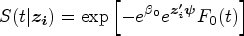
The cure-survival data is modeled by an FHC submodel connecting with an LM submodel via shared random effects. The FHC submodel is an extension of the PHC model. The PHC model’s survival function at time $T$ conditional on subject $i$ ’s covariates ${\mathit{z}}_{\mathit{i}}$ is written as

$$S(t|{\mathit{z}}_{\mathit{i}})=\exp [-e^{{\beta }_0}{e}^{{\mathit{z}}_{\mathit{i}}^{\mathbf{\prime }}\mathit{\psi }}{F}_0(t)]$$

where ${\beta }_0$ is an unknown scalar; $\mathit{\psi }$ is a $p$ -length vector of unknown regression parameters; and $F_0(t)$ is a monotone increasing function with $F_0(0)=0$ and $\underset{t\to \mathrm{\infty }}{lim}{F}_0(t)=1$ . The PHC model can be considered as a Cox PH model with a bounded baseline cumulative hazard $e^{{\beta }_0}{F}_0(t)$ and called a bounded cumulative hazard model. As $t$ goes to infinity, $F_0(t)$ tends to 1 and the cure rate can be computed as $\exp (-e^{{\beta }_0}{e}^{{\mathit{z}}_{\mathit{i}}^{\mathbf{\prime }}\mathit{\psi }})$ . Thus, $\mathit{Z}$ is regarded as the long-term covariates. With subject $i$ ’s random effects ${\mathit{\alpha }}_{\mathit{i}}$ from an LM submodel, the PHC submodel for the cure-survival data in the joint model can be defined as

$$S\{t|{\mathit{z}}_{\mathit{i}},f({\mathit{b}}_{\mathit{i}}|{\mathit{\alpha }}_{\mathit{i}})\}=\exp [-e^{{\beta }_0}{e}^{{\mathit{z}}_{\mathit{i}}^{\mathbf{\prime }}\mathit{\psi }}{e}^{{\mathit{\alpha }}_{\mathit{i}}^{\mathbf{\prime }}\mathit{\eta }}{F}_0(t)]$$

where $\mathit{\psi }$ and $\mathit{\eta }$ are two vectors of unknown regression parameters with lengths $p$ and $r^{*}$ for baseline covariates ${\mathit{z}}_{\mathit{i}}$ and random effects ${\mathit{\alpha }}_{\mathit{i}}$ , respectively.

To relax the PH assumption, we propose a new joint model, with an FHC submodel extending the above PHC submodel by raising a power on $F_0(t)$ , as follows. The survival function in our joint model (i.e., JMFHC) for subject $i$ at time $T$ conditional on covariates ${\mathit{z}}_{\mathit{i}}$ and ${\mathit{x}}_{\mathit{i}}$ and random effects ${\mathit{\alpha }}_{\mathit{i}}$ is assumed to be

$$\begin{array}{r}S\{t|{\mathit{x}}_{\mathit{i}},{\mathit{z}}_{\mathit{i}},f({\mathit{b}}_{\mathit{i}}|{\mathit{\alpha }}_{\mathit{i}})\}=\exp [-e^{{\beta }_0}{e}^{{\mathit{z}}_{\mathit{i}}^{\mathbf{\prime }}\mathit{\psi }}{e}^{{\mathit{\alpha }}_{\mathit{i}}^{\mathbf{\prime }}\mathit{\eta }}\{F_0(t){\}}^{\exp ({\mathit{x}}_{\mathit{i}}^{\mathbf{\prime }}\mathit{\gamma })}]\end{array}$$

(2)

where $\mathit{\gamma }$ is a vector of unknown regression parameters with length $q$ . Based on our JMFHC, the cure rate conditional on ${\mathit{z}}_{\mathit{i}}$ and ${\mathit{\alpha }}_{\mathit{i}}$ can be obtained as $\exp (-e^{{\beta }_0+{\mathit{z}}_{\mathit{i}}^{\mathbf{\prime }}\mathit{\psi }+{\mathit{\alpha }}_{\mathit{i}}^{\mathbf{\prime }}\mathit{\eta }})$ for subject $i$ . Since ${\mathit{\alpha }}_{\mathit{i}}$ is not observed, the cure rate at baseline given ${\mathit{z}}_{\mathit{i}}$ can be computed as

$$\begin{array}{r}{\int }_{-\mathrm{\infty }}^{\mathrm{\infty }}\exp (-e^{{\beta }_0+{\mathit{z}}_{\mathit{i}}^{\mathbf{\prime }}\mathit{\psi }+{\mathit{\alpha }}_{\mathit{i}}\mathit{\eta }})f({\mathit{\alpha }}_{\mathit{i}})d{\mathit{\alpha }}_{\mathit{i}}\end{array}$$

(3)

where $f({\mathit{\alpha }}_{\mathit{i}})$ is the multivariate normal density function of ${\mathit{\alpha }}_{\mathit{i}}$ . Parameters $\mathit{\psi }$ reflect the covariate effects ${\mathit{z}}_{\mathit{i}}$ on cure rates, and a positive ${\psi }_k$ indicates lower cure rates when the values of $z_{ik}$ increase, for $k=1,2,\dots ,p$ . On the other hand, for finite time $t$ where $F_0(t)$ is less than one, the covariates ${\mathit{x}}_{\mathit{i}}$ can contribute to the short-term survival via $F_0{(t)}^{\exp ({\mathit{x}}_{\mathit{i}}^{\mathbf{\prime }}\mathit{\gamma })}$ . Since $F_0(t)$ is fixed between 0 and 1, changes of ${\mathit{x}}_{\mathit{i}}$ values can shrink (when $x_i^{\prime }\gamma >0,\exp (x_i^{\prime }\gamma )>1$ ) or expand (when $x_i^{\prime }\gamma <0,\exp (x_i^{\prime }\gamma )<1$ ) the values $F_0(t)$ to $F_0{(t)}^{\exp ({\mathit{x}}_{\mathit{i}}^{\mathbf{\prime }}\mathit{\gamma })}$ . When $x_{ik}$ increases, a positive ${\gamma }_k$ reflects a larger short-term survival probability, $k=1,2,\dots ,q.$

When we take a logarithm of JMFHC’s cumulative hazard function, which is expressed as

$$\log [\mathrm{\Lambda }\{t|{\mathit{x}}_{\mathit{i}},{\mathit{z}}_{\mathit{i}},f({\mathit{b}}_{\mathit{i}}|{\mathit{\alpha }}_{\mathit{i}})\}]={\beta }_0+{\mathit{z}}_{\mathit{i}}^{\mathbf{\prime }}\mathit{\psi }+{\mathit{\alpha }}_{\mathit{i}}^{\mathbf{\prime }}\mathit{\eta }+\exp ({\mathit{x}}_{\mathit{i}}^{\mathbf{\prime }}\mathit{\gamma })\log \{F_0(t)\}$$

it is in the form of a linear model of $\log \{F_0(t)\}$ with ${\beta }_0+{\mathit{z}}_{\mathit{i}}^{\mathbf{\prime }}\mathit{\psi }+{\mathit{\alpha }}_{\mathit{i}}^{\mathbf{\prime }}\mathit{\eta }$ as an intercept and $\exp ({\mathit{x}}_{\mathit{i}}^{\mathbf{\prime }}\mathit{\gamma })$ as a slope. This slope term allows non-PH (including crossing) cumulative hazard functions. Changes of ${\mathit{z}}_{\mathit{i}}$ can only move the curve of $\log [\mathrm{\Lambda }\{t|{\mathit{x}}_{\mathit{i}},{\mathit{z}}_{\mathit{i}},f({\mathit{b}}_{\mathit{i}}|{\mathit{\alpha }}_{\mathit{i}})\}]$ up and down without changing its shape. Therefore, covariates following the PH assumption can only belong to ${\mathit{z}}_{\mathit{i}}$ . Depending on the effect patterns of ${\mathit{z}}_{\mathit{i}}$ and ${\mathit{x}}_{\mathit{i}}$ , covariates with the non-PH structure could be included in either only ${\mathit{x}}_{\mathit{i}}$ or both ${\mathit{z}}_{\mathit{i}}$ and ${\mathit{x}}_{\mathit{i}}$ . The term $\exp ({\mathit{x}}_{\mathit{i}}^{\mathbf{\prime }}\mathit{\gamma })$ prompts flexibility of hazard functions and feasibility of capturing the non-PH structure of covariates without a complex model. The identifiability of our proposed model is evaluated shown in Section S1 of the Supplemental Material.

3. Estimation method

The data consists of $n$ independent samples, $\{(y_i,{\delta }_i,{\mathit{z}}_i,{\mathit{x}}_i,{\mathit{\alpha }}_i),i=1,2,\dots ,n\}$ . The observed times $y_1,y_2,\dots ,y_n$ are assumed to be in ascending order for the simplicity of notations in the estimation procedure. Denote the parameters as $\mathit{\theta }=\{{\beta }_0,{\mathit{\psi }}^{\prime },{\mathit{\eta }}^{\prime },{\mathit{\gamma }}^{\prime },F_0(t),{\mathit{\zeta }}^{\prime },{\mathit{\varphi }}^{\prime },{\sigma }_1,\dots ,{\sigma }_{r^{*}},{\rho }_{jm},{\sigma }_{ϵ}{\}}^{\prime }$ , where $j,m=1,\dots ,r^{*}$ and $j\ne m$ , the observed values as $\mathit{o}=({\mathit{o}}_1^{\prime },{\mathit{o}}_2^{\prime },\dots ,{\mathit{o}}_n^{\prime }{)}^{\prime }$ with ${\mathit{o}}_{\mathit{i}}=({\mathit{z}}_{\mathit{i}}^{\prime },{\mathit{x}}_{\mathit{i}}^{\prime },{\mathit{b}}_{\mathit{i}}^{\prime },{\delta }_i,y_i{)}^{\prime }$ , for $i=1,2,\dots ,n$ , and the unobserved values or random effects as $\mathit{A}=({\mathit{\alpha }}_1^{\prime },{\mathit{\alpha }}_2^{\prime },\dots ,{\mathit{\alpha }}_n^{\prime }{)}^{\prime }$ .

With the unknown random effects, we use the expectation-maximization algorithm to estimate regression parameters $\mathit{\theta }$ . For subject $i$ , we let the hazard function at time $y_i$ be $h(y_i)$ , whose expression is shown as

$$\begin{array}{r}h(y_i)=e^{{\beta }_0}{e}^{{\mathit{z}}_{\mathit{i}}^{\mathbf{\prime }}\mathit{\psi }}{e}^{{\mathit{\alpha }}_{\mathit{i}}^{\mathbf{\prime }}\mathit{\eta }}{e}^{{\mathit{x}}_{\mathit{i}}^{\mathbf{\prime }}\mathit{\gamma }}\{F_0(y_i){\}}^{\exp ({\mathit{x}}_{\mathit{i}}^{\mathbf{\prime }}\mathit{\gamma })-1}{f}_0(y_i)\end{array}$$

(4)

The survival function at time $y_i$ is expressed as

$$\begin{array}{r}S(y_i)=\exp [-e^{{\beta }_0}{e}^{{\mathit{z}}_{\mathit{i}}^{\mathbf{\prime }}\mathit{\psi }}{e}^{{\mathit{\alpha }}_{\mathit{i}}^{\mathbf{\prime }}\mathit{\eta }}\{F_0(y_i){\}}^{\exp ({\mathit{x}}_{\mathit{i}}^{\mathbf{\prime }}\mathit{\gamma })}]\end{array}$$

(5)

The density function of ${\mathit{b}}_{\mathit{i}}$ given ${\mathit{\alpha }}_{\mathit{i}}$ is written as

$$\begin{array}{rl}f({\mathit{b}}_{\mathit{i}}|{\mathit{\alpha }}_{\mathit{i}})=& (2\pi {\sigma }_{ϵ}^2{)}^{-\frac{n_i}{2}}\exp [-\frac{1}{2{\sigma }_{ϵ}^2}\{{\mathit{b}}_{\mathit{i}}-{\mathit{H}}_{\mathit{i}}\mathit{\zeta }-{\mathit{D}}_{\mathit{i}}\mathbf{(}{\mathit{t}}_{\mathit{i}}\mathbf{)}\mathit{\varphi }-{\mathit{Q}}_{\mathit{i}}\mathbf{(}{\mathit{t}}_{\mathit{i}}\mathbf{)}{\mathit{\alpha }}_{\mathit{i}}{\}}^{\prime }\{{\mathit{b}}_{\mathit{i}}-{\mathit{H}}_{\mathit{i}}\mathit{\zeta }-{\mathit{D}}_{\mathit{i}}\mathbf{(}{\mathit{t}}_{\mathit{i}}\mathbf{)}\mathit{\varphi }-{\mathit{Q}}_{\mathit{i}}\mathbf{(}{\mathit{t}}_{\mathit{i}}\mathbf{)}{\mathit{\alpha }}_{\mathit{i}}\}]\end{array}$$

(6)

The density function of ${\mathit{\alpha }}_{\mathit{i}}$ is expressed as

$$\begin{array}{r}f({\mathit{\alpha }}_{\mathit{i}})={\left(2\pi \right)}^{-\frac{r^{*}}{2}}|\mathbf{\Sigma }{|}^{-\frac{1}{2}}\exp (-\frac{1}{2}{\mathit{\alpha }}_{\mathit{i}}^{\prime }{\mathbf{\Sigma }}^{-1}{\mathit{\alpha }}_{\mathit{i}})\end{array}$$

(7)

With equations (4)–(7), the complete-data likelihood function of JMFHC is written as

$$\begin{array}{r}{L}_c(\mathit{\theta };\mathit{o},\mathit{A})=\prod _{i=1}^n{L}_{ic}(\mathit{\theta };{\mathit{o}}_{\mathit{i}},{\mathit{\alpha }}_{\mathit{i}})=\prod _{i=1}^n\{h(y_i){\}}^{{\delta }_i}S(y_i)f({\mathit{b}}_{\mathit{i}}|{\mathit{\alpha }}_{\mathit{i}})f({\mathit{\alpha }}_{\mathit{i}})\end{array}$$

(8)

Suppose $\mathit{A}$ is observed. The full likelihood function is written as

$$\begin{array}{r}L(\mathit{\theta };\mathit{o},\mathit{A})=\prod _{i=1}^n{L}_i(\mathit{\theta };{\mathit{o}}_{\mathit{i}},{\mathit{\alpha }}_{\mathit{i}})=\prod _{i=1}^n\{h(y_i){\}}^{{\delta }_i}S(y_i)f({\mathit{b}}_{\mathit{i}}|{\mathit{\alpha }}_{\mathit{i}})\end{array}$$

(9)

With the complex form of equation (9), subject $i$ ’s marginal likelihood function is expressed as

$$\begin{array}{r}{L}_i(\mathit{\theta };{\mathit{o}}_{\mathit{i}})={\int }_{-\mathrm{\infty }}^{\mathrm{\infty }}{L}_i(\mathit{\theta };{\mathit{o}}_{\mathit{i}},{\mathit{\alpha }}_{\mathit{i}})f({\mathit{\alpha }}_{\mathit{i}})d{\mathit{\alpha }}_{\mathit{i}}\end{array}$$

(10)

The integral in equation (10) does not have a closed form. In such case, the posterior distribution function of subject $i$ ’s random effects ${\mathit{\alpha }}_{\mathit{i}}$ with equation (10) as the denominator, which is expressed as

$$\begin{array}{r}{f}_{{\mathit{\alpha }}_{\mathit{i}}|{\mathit{o}}_{\mathit{i}}}({\mathit{\alpha }}_{\mathit{i}};\mathit{\theta })=\frac{L_i(\mathit{\theta };{\mathit{o}}_{\mathit{i}},{\mathit{\alpha }}_{\mathit{i}})f({\mathit{\alpha }}_{\mathit{i}})}{L_i(\mathit{\theta };{\mathit{o}}_{\mathit{i}})}\propto L_i(\mathit{\theta };{\mathit{o}}_{\mathit{i}},{\mathit{\alpha }}_{\mathit{i}})f({\mathit{\alpha }}_{\mathit{i}})\end{array}$$

(11)

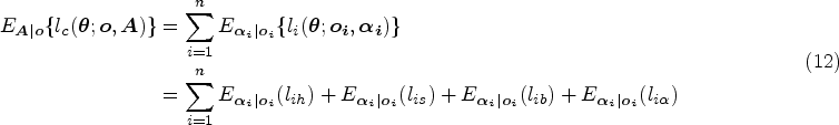
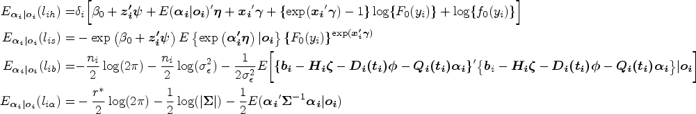
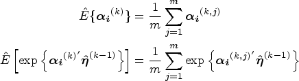
does not have a closed form. We derive the expectation of the complete-data log-likelihood function with respect to the posterior distribution of random effects $\mathit{A}$ , which is written as

$$\begin{array}{r}\begin{array}{rl}{E}_{\mathit{A}|\mathit{o}}\{l_c(\mathit{\theta };\mathit{o},\mathit{A})\}& =\sum _{i=1}^n{E}_{{\mathit{\alpha }}_{\mathit{i}}|{\mathit{o}}_{\mathit{i}}}\{l_i(\mathit{\theta };{\mathit{o}}_{\mathit{i}},{\mathit{\alpha }}_{\mathit{i}})\}\\ & =\sum _{i=1}^n{E}_{{\mathit{\alpha }}_{\mathit{i}}|{\mathit{o}}_{\mathit{i}}}(l_{ih})+E_{{\mathit{\alpha }}_{\mathit{i}}|{\mathit{o}}_{\mathit{i}}}(l_{is})+E_{{\mathit{\alpha }}_{\mathit{i}}|{\mathit{o}}_{\mathit{i}}}(l_{ib})+E_{{\mathit{\alpha }}_{\mathit{i}}|{\mathit{o}}_{\mathit{i}}}(l_{i\alpha })\end{array}\end{array}$$

(12)

where

$$\begin{array}{rl}{E}_{{\mathit{\alpha }}_{\mathit{i}}|{\mathit{o}}_{\mathit{i}}}(l_{ih})=& {\delta }_i[{\beta }_0+{\mathit{z}}_{\mathit{i}}^{\mathbf{\prime }}\mathit{\psi }+E({\mathit{\alpha }}_{\mathit{i}}|{\mathit{o}}_{\mathit{i}}{)}^{\prime }\mathit{\eta }+{\mathit{x}}_{\mathit{i}}^{\prime }\mathit{\gamma }+\{\exp ({\mathit{x}}_{\mathit{i}}^{\prime }\mathit{\gamma })-1\}\log \{F_0(y_i)\}+\log \{f_0(y_i)\}]\\ E_{{\mathit{\alpha }}_{\mathit{i}}|{\mathit{o}}_{\mathit{i}}}(l_{is})=& -\exp ({\beta }_0+{\mathit{z}}_{\mathit{i}}^{\mathbf{\prime }}\mathit{\psi })E\left\{\exp \left({\mathit{\alpha }}_{\mathit{i}}^{\mathbf{\prime }}\mathit{\eta }\right)|{\mathit{o}}_{\mathit{i}}\right\}\{F_0(y_i){\}}^{\exp ({\mathit{x}}_{\mathit{i}}^{\mathbf{\prime }}\mathit{\gamma })}\\ E_{{\mathit{\alpha }}_{\mathit{i}}|{\mathit{o}}_{\mathit{i}}}(l_{ib})=& -\frac{n_i}{2}\log (2\pi )-\frac{n_i}{2}\log ({\sigma }_{ϵ}^2)-\frac{1}{2{\sigma }_{ϵ}^2}E[\{{\mathit{b}}_{\mathit{i}}-{\mathit{H}}_{\mathit{i}}\mathit{\zeta }-{\mathit{D}}_{\mathit{i}}\mathbf{(}{\mathit{t}}_{\mathit{i}}\mathbf{)}\mathit{\varphi }-{\mathit{Q}}_{\mathit{i}}\mathbf{(}{\mathit{t}}_{\mathit{i}}\mathbf{)}{\mathit{\alpha }}_{\mathit{i}}{\}}^{\prime }\{{\mathit{b}}_i-{\mathit{H}}_{\mathit{i}}\mathit{\zeta }-{\mathit{D}}_{\mathit{i}}\mathbf{(}{\mathit{t}}_{\mathit{i}}\mathbf{)}\mathit{\varphi }-{\mathit{Q}}_{\mathit{i}}\mathbf{(}{\mathit{t}}_{\mathit{i}}\mathbf{)}{\mathit{\alpha }}_{\mathit{i}}\}|{\mathit{o}}_{\mathit{i}}]\\ E_{{\mathit{\alpha }}_{\mathit{i}}|{\mathit{o}}_{\mathit{i}}}(l_{i\alpha })=& -\frac{r^{*}}{2}\log (2\pi )-\frac{1}{2}\log (|\mathbf{\Sigma }|)-\frac{1}{2}E({\mathit{\alpha }}_{\mathit{i}}^{\prime }{\mathbf{\Sigma }}^{-1}{\mathit{\alpha }}_{\mathit{i}}|{\mathit{o}}_{\mathit{i}})\end{array}$$

Hence, the MCEM algorithm is implemented for parameter estimation. In the E step, the expectation of the complete-data log-likelihood function with respect to the posterior distribution of random effects is numerically obtained through Monte Carlo simulations. More specifically, an adaptive Metropolis (AM) algorithm ⁵⁸ is implemented to generate samples of subject-specific random effects. In the M step, the parameters $\mathit{\theta }$ are updated by maximizing the expected log-likelihood function obtained in the E step.

Let $k$ be the number of iterations, where $k=0,1,2,\dots$ . We set $k=0$ as the initial step (Step 1 below). The E step of the MCEM algorithm is shown in Step 2, and the M step is presented as Steps 3–5. Steps 2–5 are considered as one iteration of estimation. A parameter value at the $k_{th}$ iteration has a superscript $(k)$ on the corresponding notation. The estimation procedure is outlined as follows:

• Step 1:

Initial values of regression parameters in two submodels of JMFHC are obtained.

In the LM submodel, we use the restricted maximum likelihood ⁵⁹ to estimate parameters $\mathit{\zeta },\mathit{\varphi },\mathbf{\Sigma },$ and ${\sigma }_{ϵ}$ , and predict subjects’ random effects denoted as ${\hat{\mathit{A}}}^{(0)}$ .

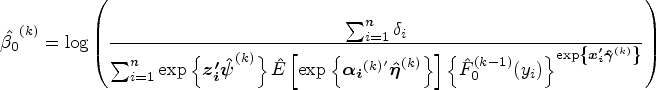
In the cure submodel, given ${\hat{\mathit{A}}}^{(0)}$ , we determine the initial values of parameters and $F_0(t)$ . First, $\mathit{\gamma }$ is set as $\mathbf{0}$ . ${\hat{\mathit{\psi }}}^{(0)}{\hat{\mathit{\eta }}}^{(0)}{\hat{\mathit{\psi }}}^{(0)}{\hat{\mathit{\eta }}}^{(0)}$ are estimated via the maximum partial likelihood estimation method under a standard Cox PH model. Denote the Breslow estimator as ${\hat{M}}_0(t)=\sum _{i:y_i\le t}{\hat{m}}_0(y_i)$ , where ${\hat{m}}_0(y_i)$ is the baseline hazard function at time $y_i$ . Based on the Breslow estimator, the initial value of ${\beta }_0$ is computed as ${\widehat{{\beta }_0}}^{(0)}=\log \{{\hat{M}}_0(y_n)\}$ . The initial values of $F_0(t)$ are derived as ${\hat{F}}_0^{(0)}(y_i)=\frac{{\hat{M}}_0(y_i)}{{\hat{M}}_0(y_n)},$ $i=1,2,\dots ,n.$ The corresponding point mass of $F_0(y_i)$ is computed as $f_0(y_i)=\{F_0(y_{i+1})-F_0(y_i)\}I({\delta }_i=1)$ for subject $i$ , where $I(\cdot )$ is an indicator function. Given the rest of initial values of parameters ${\hat{\mathit{\theta }}}^{(0)}$ , we obtain ${\hat{\mathit{\gamma }}}^{(0)}$ by maximizing the logarithm of equation (9).

Step 2:

At iteration $k$ , where $k=1,2,\dots$ , the AM algorithm ⁵⁸ is implemented to generate chains of the random effects ${\mathit{A}}^{(k)}$ . The target distribution for the Monte Carlo simulations is shown in equation (11) with the latest estimated parameters ${\hat{\mathit{\theta }}}^{(k-1)}$ . The details of the AM algorithm are shown in Section S2 of the Supplemental Material. Suppose the number of samples in subject $i$ ’s final chain is $m$ after burn-in and thinning. The expectations of sufficient statistics involving subject $i$ ’s random effects can be computed with sampled random effects, such as

$$\begin{array}{rl}\hat{E}\{{\mathit{\alpha }}_{\mathit{i}}^{(k)}\}& =\frac{1}{m}\sum _{j=1}^m{\mathit{\alpha }}_{\mathit{i}}^{(k,j)}\\ \hat{E}\left[\exp \left\{{\mathit{\alpha }}_{\mathit{i}}^{{(k)}^{\prime }}{\hat{\mathit{\eta }}}^{(k-1)}\right\}\right]& =\frac{1}{m}\sum _{j=1}^m\exp \left\{{\mathit{\alpha }}_{\mathit{i}}^{(k,j{)}^{\prime }}{\hat{\mathit{\eta }}}^{(k-1)}\right\}\end{array}$$

In the following steps, all the parameters $\mathit{\theta }$ are updated by maximizing equation (12) with all the latest estimated parameters.

Step 3:

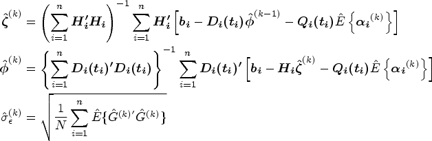
The parameters in the longitudinal submodel $\mathit{\zeta },\mathit{\varphi },\mathbf{\Sigma }$ , and ${\sigma }_{ϵ}$ are estimated by maximizing equation (12). By taking the partial derivatives of $\sum _i^n{\hat{E}}_{{\mathit{\alpha }}_{\mathit{i}}|{\mathit{o}}_{\mathit{i}}}(l_{ib})$ with respect to $\mathit{\zeta },\mathit{\varphi }$ , and ${\sigma }_{ϵ}$ with the equations set to zero, we obtain the estimators of $\mathit{\zeta },\mathit{\varphi }$ , and ${\sigma }_{ϵ}$ as follows:

$$\begin{array}{rl}{\hat{\mathit{\zeta }}}^{(k)}& ={\left(\sum _{i=1}^n{\mathit{H}}_{\mathit{i}}^{\mathbf{\prime }}{\mathit{H}}_{\mathit{i}}\right)}^{-1}\sum _{i=1}^n{\mathit{H}}_{\mathit{i}}^{\mathbf{\prime }}[{\mathit{b}}_{\mathit{i}}-{\mathit{D}}_{\mathit{i}}\mathbf{(}{\mathit{t}}_{\mathit{i}}\mathbf{)}{\hat{\mathit{\varphi }}}^{(k-1)}-{\mathit{Q}}_{\mathit{i}}\mathbf{(}{\mathit{t}}_{\mathit{i}}\mathbf{)}\hat{E}\left\{{\mathit{\alpha }}_{\mathit{i}}^{(k)}\right\}]\\ {\hat{\mathit{\varphi }}}^{(k)}& ={\left\{\sum _{i=1}^n{\mathit{D}}_{\mathit{i}}\mathbf{(}{\mathit{t}}_{\mathit{i}}{\mathbf{)}}^{\mathbf{\prime }}{\mathit{D}}_{\mathit{i}}\mathbf{(}{\mathit{t}}_{\mathit{i}}\mathbf{)}\right\}}^{-1}\sum _{i=1}^n{\mathit{D}}_{\mathit{i}}\mathbf{(}{\mathit{t}}_{\mathit{i}}{\mathbf{)}}^{\mathbf{\prime }}[{\mathit{b}}_{\mathit{i}}-{\mathit{H}}_{\mathit{i}}{\hat{\mathit{\zeta }}}^{(k)}-{\mathit{Q}}_{\mathit{i}}\mathbf{(}{\mathit{t}}_{\mathit{i}}\mathbf{)}\hat{E}\left\{{\mathit{\alpha }}_{\mathit{i}}^{(k)}\right\}]\\ {\hat{\sigma }}_{ϵ}^{(k)}& =\sqrt{\frac{1}{N}\sum _{i=1}^n\hat{E}\{{\hat{G}}^{{(k)}^{\prime }}{\hat{G}}^{(k)}\}}\end{array}$$

where ${\hat{G}}^{(k)}={\mathit{b}}_{\mathit{i}}-{\mathit{H}}_{\mathit{i}}{\hat{\mathit{\zeta }}}^{(k)}-{{\mathit{D}}_{\mathit{i}}\mathbf{(}{\mathit{t}}_{\mathit{i}}\mathbf{)}\hat{\mathit{\varphi }}}^{(k)}-{\mathit{Q}}_{\mathit{i}}\mathbf{(}{\mathit{t}}_{\mathit{i}}\mathbf{)}{\mathit{\alpha }}_{\mathit{i}}^{(k)}$ . Similarly, we solve $\mathrm{\partial }\sum _i^n{\hat{E}}_{{\mathit{\alpha }}_{\mathit{i}}|{\mathit{o}}_{\mathit{i}}}(l_{i\alpha })/\mathrm{\partial }\mathbf{\Sigma }=0$ and obtain ${\hat{\mathbf{\Sigma }}}^{(k)}=\frac{1}{n}\sum _{i=1}^n\hat{E}\{{\mathit{\alpha }}_{\mathit{i}}^{(k)}{\mathit{\alpha }}_{\mathit{i}}^{{(k)}^{\prime }}\}.$

Step 4:

The parameters in the cure submodel $\mathit{\psi }$ , $\mathit{\eta }$ , and $\mathit{\gamma }$ are estimated by maximizing equation (12) (using R function optim), which can be simplified as $E_{\mathit{A}|\mathit{o}}\{l(\mathit{\psi },\mathit{\eta },\mathit{\gamma })\}=\sum _{i=1}^n{E}_{{\mathit{\alpha }}_{\mathit{i}}|{\mathit{o}}_{\mathit{i}}}(l_{ih})+E_{{\mathit{\alpha }}_{\mathit{i}}|{\mathit{o}}_{\mathit{i}}}(l_{is}).$ With ${\hat{\mathit{\psi }}}^{(k)}$ , ${\hat{\mathit{\eta }}}^{(k)}$ , and ${\hat{\mathit{\gamma }}}^{(k)}$ , the estimator ${\widehat{{\beta }_0}}^{(k)}$ is obtained by solving $\mathrm{\partial }{l}_c/\mathrm{\partial }{\beta }_0=0$ , which is written as

$${\widehat{{\beta }_0}}^{(k)}=\log \left(\frac{\sum _{i=1}^n{\delta }_i}{\sum _{i=1}^n\exp \left\{{\mathit{z}}_{\mathit{i}}^{\mathbf{\prime }}{\hat{\mathit{\psi }}}^{(k)}\right\}\hat{E}\left[\exp \left\{{\mathit{\alpha }}_{\mathit{i}}^{{(k)}^{\prime }}{\hat{\mathit{\eta }}}^{(k)}\right\}\right]{\{{\hat{F}}_0^{(k-1)}(y_i)\}}^{\exp \left\{{\mathit{x}}_{\mathit{i}}^{\mathbf{\prime }}{\hat{\mathit{\gamma }}}^{(k)}\right\}}}\right)$$

Step 5:

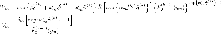
The function ${\hat{F}}_0^{(k)}(t)$ is updated. We implement the Lagrange multiplier method to derive jump sizes $f_0(y_i)$ first, $i=1,2,\dots n$ , under the constraint $\sum _{i=1}^n{f}_0(y_i)=1$ . Similar methods have been applied in the estimation of other cure models^60,61 and a joint model of longitudinal cure-survival data. ⁵² Define

$$\begin{array}{r}G\{f_0(y_1),\dots ,f_0(y_n),\lambda \}=E_{\mathit{A}|\mathit{o}}[l_c\{f_0(y_1),\dots ,f_0(y_n)\}]-\lambda \{\sum _{i=1}^n{f}_0(y_i)-1\}\end{array}$$

(13)

where $\lambda$ is the Lagrange multiplier and $E_{\mathit{A}|\mathit{o}}[l_c\{f_0(y_1),\dots ,f_0(y_n)\}]$ is equation (12) with each $F_0(y_i)$ replaced by $\sum _{j=1}^i{f}_0(y_j)$ . By maximizing equation (13), we obtain the estimator of $f_0^{(k)}(y_i)$ at the $k_{th}$ iteration, which is expressed as

$$\begin{array}{r}{\hat{f}}_0^{(k)}(y_i|\lambda )=\frac{{\delta }_i}{\sum _{m=i}^n(W_m-V_m)+\lambda }\end{array}$$

(14)

where

$$\begin{array}{rl}{W}_m& =\exp \{{\widehat{{\beta }_0}}^{(k)}+{\mathit{z}}_{\mathit{m}}^{\mathbf{\prime }}{\hat{\mathit{\psi }}}^{(k)}+{\mathit{x}}_{\mathit{m}}^{\mathbf{\prime }}{\hat{\mathit{\gamma }}}^{(k)}\}\hat{E}\left[\exp \left\{{\mathit{\alpha }}_{\mathit{m}}^{{(k)}^{\prime }}{\hat{\mathit{\eta }}}^{(k)}\right\}\right]{\{{\hat{F}}_0^{(k-1)}(y_m)\}}^{\exp \left\{{\mathit{x}}_{\mathit{m}}^{\mathbf{\prime }}{\hat{\mathit{\gamma }}}^{(k)}\right\}-1}\\ V_m& =\frac{{\delta }_m[\exp \{{\mathit{x}}_{\mathit{m}}^{\mathbf{\prime }}{\hat{\mathit{\gamma }}}^{(k)}\}-1]}{{\hat{F}}_0^{(k-1)}(y_m)}\end{array}$$

When ${\delta }_i=0$ , ${\hat{f}}_0^{(k)}(y_i|\lambda )=0$ . We solve for $\lambda$ by using $\sum _{i=1}^n{\hat{f}}^{(k)}(y_i|\lambda )=1$ since $\sum _{i=1}^n{\hat{f}}^{(k)}(y_i|\lambda )$ is a monotone function of $\lambda$ . An updated estimator ${\hat{f}}_0^{(k)}(y_i|\hat{\lambda })$ can be obtained with the estimate $\hat{\lambda }$ . We update the function $F_0(t)$ via ${\hat{F}}_0^{(k)}(t)=\sum _{i:y_i\le t}{\hat{f}}_0^{(k)}(y_i|\hat{\lambda }).$

Steps 2–5 are iterated until convergence of estimated parameters $\hat{\mathit{\theta }}$ . Based on our estimation method due to the constraint of $F_0(y_n)$ ’s jump sizes, $\sum _{i=1}^n{\hat{f}}^{(k)}(y_i|\lambda )$ =1, censored patients whose censoring times are greater than or equal to the maximum of all event times are considered to be cured. This assumption ensures the cure submodel identifiability, which is also used by other cure models.^{11,21,22,28,30} The proof of identifiability for our proposed model is presented in Section S1 of the Supplemental Material.

We apply a jackknife resampling method to compute the standard errors of $\mathit{\theta }$ . The non-parametric bootstrap cannot achieve the covariance estimation for our model since the ties from the resampling with replacement would make the cure model’s fitting difficult. The jackknife resampling method removes one subject’s record each time, and the same estimation procedure for point estimation presented above is used on the resampled data. The standard errors of parameter estimators $\mathit{\theta }$ can be computed as $\sqrt{\frac{n-1}{n}\sum _{i=1}^n\{{\hat{\mathit{\theta }}}_{(i)}-{\hat{\mathit{\theta }}}_{(.)}{\}}^2},$ where ${\hat{\mathit{\theta }}}_{(1)},{\hat{\mathit{\theta }}}_{(2)},\dots ,{\hat{\mathit{\theta }}}_{(n)}$ are the estimated parameters from model fitting on $n$ different resampled data sets, and ${\hat{\mathit{\theta }}}_{(.)}=\frac{1}{n}\sum _{i=1}^n{\hat{\mathit{\theta }}}_{(i)}$ . The point estimation and standard error estimation for our comparison model JMPHC are the same as JMFHC except that $\mathit{\gamma }$ is set as $\mathbf{0}$ for JMPHC throughout the estimation.

4. Simulation studies

We performed simulation studies under four scenarios to assess the performance and estimation method of the proposed model JMFHC and compared it with JMPHC. These two models consisted of an LM submodel as the longitudinal submodel and cure submodels with flexible patterns of hazard functions (i.e., JMFHC) and PH structure (i.e., JMPHC), respectively. Scenarios 1 and 4 had baseline covariates violating the PH assumption with crossing. Under scenario 2, baseline covariates had non-crossing survival functions, but violated the PH assumption. Scenario 3 followed the PH assumption and thus satisfied the assumption of JMPHC. Compared to scenario 4, scenarios 1–3 have smaller censoring rates and larger cure rates.

We conducted 500 runs for each scenario with a sample size of 500. In each simulation scenario, a data set was generated from JMFHC based on equations (1) and (2). We generated a binary baseline variable $X_1$ taking 0 or 1 with equal probability. In the simulations, we considered a linear trajectory of longitudinal biomarker measurements. The function of subject $i$ ’s biomarker measurement at time $t_{ij}$ was written as

$$b_{ij}(t_{ij})={\varphi }_0+{\varphi }_1{t}_{ij}+{\alpha }_{i0}+{\alpha }_{i1}{t}_{ij}+{ϵ}_{ij},i=1,2,\dots ,500,j=1,2,\dots ,n_i$$

The fixed population intercept and slope $({\varphi }_0,{\varphi }_1{)}^{\prime }$ were set as $(5,-1{)}^{\prime }$ . The subject-specific random intercept and slope were generated from a bivariate normal distribution with mean $\mathbf{0}$ and a covariance matrix with ${\sigma }_1=0.8,{\sigma }_2=0.5$ , and $\rho =0$ . The standard deviation of the measurement errors was set as ${\sigma }_{ϵ}=1$ . The prespecified measurement time points were set as $0,1,\dots ,50$ .

In the underlying JMFHC’s cure submodel with the form of equation (2), we let ${\mathit{z}}_{\mathit{i}}={\mathit{x}}_{\mathit{i}}=x_{i1}$ and ${\mathit{\alpha }}_{\mathit{i}}=({\alpha }_{i0},{\alpha }_{i1}{)}^{\prime }$ , and the FHC submodel was written as

$$\begin{array}{r}S(t|x_{i1},{\alpha }_{i0},{\alpha }_{i1})=\exp [-\exp ({\beta }_0+{\psi }_1{x}_{i1}+{\eta }_1{\alpha }_{i0}+{\eta }_2{\alpha }_{i1})\{F_0(t){\}}^{\exp ({\gamma }_1{x}_{i1})}]\end{array}$$

(15)

The true $F_0(t)$ was set as $1-\exp \{-(t/20{)}^8\}$ . We considered $X_1$ with a non-PH structure under scenarios 1, 2, and 4 and a PH structure under scenario 3. The true values of ${\beta }_0,{\psi }_1,{\eta }_1,{\eta }_2,$ and ${\gamma }_1$ were set as $(-0.1,1,0.5,-0.7,0.8)$ for scenarios 1 and 4, $(1,-1,0.5,-0.7,0.8)$ for scenario 2, and $(1,-1,0.5,-0.7,0)$ for scenario 3.

The function of survival times was derived from equation (15), which is expressed as

$$T_i=F_0^{-1}([-\log (u_i)\exp \{-({\beta }_0+{\psi }_1{x}_{i1}+{\eta }_1{\alpha }_{i0}+{\eta }_2{\alpha }_{i1})\}{]}^{\exp (-{\gamma }_1{x}_{i1})}),i=1,\dots ,500$$

where $F_0^{-1}(\cdot )$ was the inverse of $F_0(t)$ , and $u_i$ followed a standard uniform distribution. For subject $i$ with the value of $[-\log (u_i)\exp \{-({\beta }_0+{\psi }_1{x}_{i1}+{\eta }_1{\alpha }_{i0}+{\eta }_2{\alpha }_{i1})\}{]}^{\exp (-{\gamma }_1{x}_{i1})}$ less than or equal to 1, its survival time was $T_i$ . Otherwise, this patient’s survival time was set as 99999, which meant that he or she was cured. The censoring times $C$ were generated from a continuous uniform distribution with parameters of $U(10,60)$ under scenarios 1–3 and $U(10,30)$ under scenario 4. For each subject, we discarded the generated biomarker values after its observed survival time. The mean number of subjects’ biomarker measurements per person was about 22 under scenarios 1–3 and 18 under scenario 4. Under scenarios 1–4, the means of censoring rates were 38.9%, 35.8%, 34.5%, and 58.3%, respectively, and the percentages of cured ones among these censored subjects were 67.4%, 66.1%, 68.5%, and 45.0%, respectively.

The convergence criteria for $\mathit{\theta }$ except $F_0(t)$ were set to be the relative differences between previous and current estimates (e.g., $|({\beta }_0^{(k)}-{\beta }_0^{(k-1)})/{\beta }_0^{(k-1)}|$ ) less than 0.002 or the absolute differences (e.g., $|{\beta }_0^{(k)}-{\beta }_0^{(k-1)}|$ ) less than 0.001. The convergence criterion for $F_0(t)$ was the average of the relative differences between previous and current estimates less than 0.005 or the average of absolute differences less than 0.002. The maximum number of estimation iterations was set as 200. In the step of the AM algorithm, the final chain for each subject was obtained by thinning 10,000 draws by five after 1,000 draws of burn-in. With the MCEM algorithm, the convergence rates for JMFHC were 100% under simulation scenarios 2 and 3 and 98.2% under scenarios 1 and 4. The convergence rates for JMPHC were 100% under all scenarios.

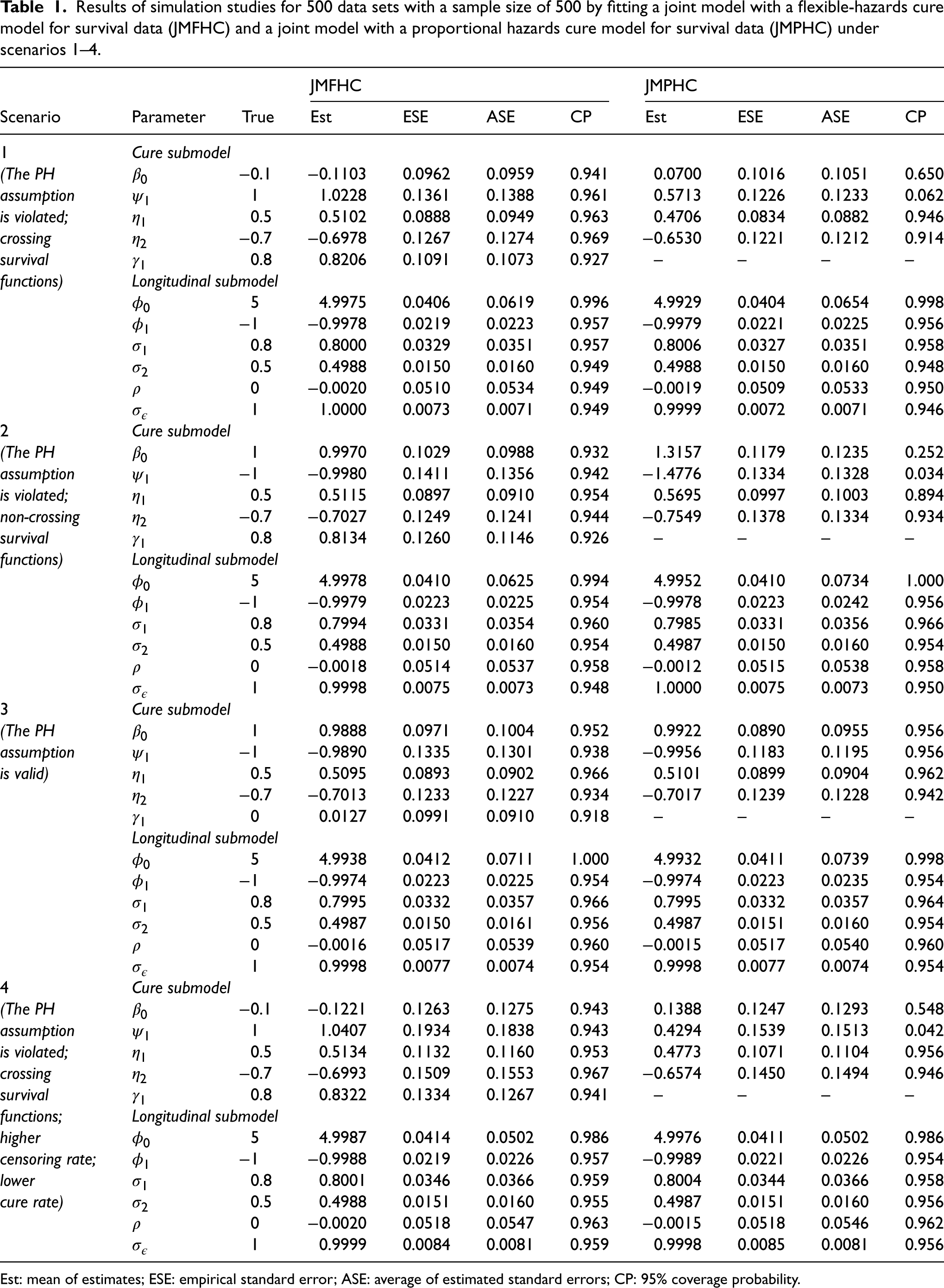
Our proposed model JMFHC showed unbiased regression parameter estimates and estimated standard errors matching the empirical ones. Table 1 presents all regression parameters’ means of estimates, empirical standard errors (ESEs), averages of estimated standard errors (ASEs), and 95% coverage probabilities (CPs) from JMFHC and JMPHC under four scenarios. Across four scenarios, JMFHC performed well with means of estimates close to the true values of the regression parameters from two submodels. Also, these regression parameters’ ASEs agreed with their corresponding ESEs. All empirical CPs were near the nominal level of 95%. On the other hand, when the PH assumption was violated under scenarios 1, 2, and 4, JMPHC had the means of estimated parameters from its cure submodels, especially ${\hat{\beta }}_0$ and ${\hat{\psi }}_1$ , biased from the true values, even though its means of estimated regression parameters from LM submodels were close to the true values. Not all cure-survival parameters’ CPs were near the nominal level of 95%. Under scenario 3, JMPHC had the means of estimated parameters from two submodels close to the true values since the PH assumption was satisfied, and the 95% CPs were around the nominal level. ASEs of regression parameters estimated by JMPHC agreed with the corresponding ESEs under all four scenarios.

Table 1.

Results of simulation studies for 500 data sets with a sample size of 500 by fitting a joint model with a flexible-hazards cure model for survival data (JMFHC) and a joint model with a proportional hazards cure model for survival data (JMPHC) under scenarios 1–4.

			JMFHC				JMPHC
Scenario	Parameter	True	Est	ESE	ASE	CP	Est	ESE	ASE	CP
1	Cure submodel
(The PH	${\beta }_0$	−0.1	−0.1103	0.0962	0.0959	0.941	0.0700	0.1016	0.1051	0.650
assumption	${\psi }_1$	1	1.0228	0.1361	0.1388	0.961	0.5713	0.1226	0.1233	0.062
is violated;	${\eta }_1$	0.5	0.5102	0.0888	0.0949	0.963	0.4706	0.0834	0.0882	0.946
crossing	${\eta }_2$	−0.7	−0.6978	0.1267	0.1274	0.969	−0.6530	0.1221	0.1212	0.914
survival	${\gamma }_1$	0.8	0.8206	0.1091	0.1073	0.927	–	–	–	–
functions)	Longitudinal submodel
	${\varphi }_0$	5	4.9975	0.0406	0.0619	0.996	4.9929	0.0404	0.0654	0.998
	${\varphi }_1$	−1	−0.9978	0.0219	0.0223	0.957	−0.9979	0.0221	0.0225	0.956
	${\sigma }_1$	0.8	0.8000	0.0329	0.0351	0.957	0.8006	0.0327	0.0351	0.958
	${\sigma }_2$	0.5	0.4988	0.0150	0.0160	0.949	0.4988	0.0150	0.0160	0.948
	$\rho$	0	−0.0020	0.0510	0.0534	0.949	−0.0019	0.0509	0.0533	0.950
	${\sigma }_{ϵ}$	1	1.0000	0.0073	0.0071	0.949	0.9999	0.0072	0.0071	0.946
2	Cure submodel
(The PH	${\beta }_0$	1	0.9970	0.1029	0.0988	0.932	1.3157	0.1179	0.1235	0.252
assumption	${\psi }_1$	−1	−0.9980	0.1411	0.1356	0.942	−1.4776	0.1334	0.1328	0.034
is violated;	${\eta }_1$	0.5	0.5115	0.0897	0.0910	0.954	0.5695	0.0997	0.1003	0.894
non-crossing	${\eta }_2$	−0.7	−0.7027	0.1249	0.1241	0.944	−0.7549	0.1378	0.1334	0.934
survival	${\gamma }_1$	0.8	0.8134	0.1260	0.1146	0.926	–	–	–	–
functions)	Longitudinal submodel
	${\varphi }_0$	5	4.9978	0.0410	0.0625	0.994	4.9952	0.0410	0.0734	1.000
	${\varphi }_1$	−1	−0.9979	0.0223	0.0225	0.954	−0.9978	0.0223	0.0242	0.956
	${\sigma }_1$	0.8	0.7994	0.0331	0.0354	0.960	0.7985	0.0331	0.0356	0.966
	${\sigma }_2$	0.5	0.4988	0.0150	0.0160	0.954	0.4987	0.0150	0.0160	0.954
	$\rho$	0	−0.0018	0.0514	0.0537	0.958	−0.0012	0.0515	0.0538	0.958
	${\sigma }_{ϵ}$	1	0.9998	0.0075	0.0073	0.948	1.0000	0.0075	0.0073	0.950
3	Cure submodel
(The PH	${\beta }_0$	1	0.9888	0.0971	0.1004	0.952	0.9922	0.0890	0.0955	0.956
assumption	${\psi }_1$	−1	−0.9890	0.1335	0.1301	0.938	−0.9956	0.1183	0.1195	0.956
is valid)	${\eta }_1$	0.5	0.5095	0.0893	0.0902	0.966	0.5101	0.0899	0.0904	0.962
	${\eta }_2$	−0.7	−0.7013	0.1233	0.1227	0.934	−0.7017	0.1239	0.1228	0.942
	${\gamma }_1$	0	0.0127	0.0991	0.0910	0.918	–	–	–	–
	Longitudinal submodel
	${\varphi }_0$	5	4.9938	0.0412	0.0711	1.000	4.9932	0.0411	0.0739	0.998
	${\varphi }_1$	−1	−0.9974	0.0223	0.0225	0.954	−0.9974	0.0223	0.0235	0.954
	${\sigma }_1$	0.8	0.7995	0.0332	0.0357	0.966	0.7995	0.0332	0.0357	0.964
	${\sigma }_2$	0.5	0.4987	0.0150	0.0161	0.956	0.4987	0.0151	0.0160	0.954
	$\rho$	0	−0.0016	0.0517	0.0539	0.960	−0.0015	0.0517	0.0540	0.960
	${\sigma }_{ϵ}$	1	0.9998	0.0077	0.0074	0.954	0.9998	0.0077	0.0074	0.954
4	Cure submodel
(The PH	${\beta }_0$	−0.1	−0.1221	0.1263	0.1275	0.943	0.1388	0.1247	0.1293	0.548
assumption	${\psi }_1$	1	1.0407	0.1934	0.1838	0.943	0.4294	0.1539	0.1513	0.042
is violated;	${\eta }_1$	0.5	0.5134	0.1132	0.1160	0.953	0.4773	0.1071	0.1104	0.956
crossing	${\eta }_2$	−0.7	−0.6993	0.1509	0.1553	0.967	−0.6574	0.1450	0.1494	0.946
survival	${\gamma }_1$	0.8	0.8322	0.1334	0.1267	0.941	–	–	–	–
functions;	Longitudinal submodel
higher	${\varphi }_0$	5	4.9987	0.0414	0.0502	0.986	4.9976	0.0411	0.0502	0.986
censoring rate;	${\varphi }_1$	−1	−0.9988	0.0219	0.0226	0.957	−0.9989	0.0221	0.0226	0.954
lower	${\sigma }_1$	0.8	0.8001	0.0346	0.0366	0.959	0.8004	0.0344	0.0366	0.958
cure rate)	${\sigma }_2$	0.5	0.4988	0.0151	0.0160	0.955	0.4987	0.0151	0.0160	0.956
	$\rho$	0	−0.0020	0.0518	0.0547	0.963	−0.0015	0.0518	0.0546	0.962
	${\sigma }_{ϵ}$	1	0.9999	0.0084	0.0081	0.959	0.9998	0.0085	0.0081	0.956

Est: mean of estimates; ESE: empirical standard error; ASE: average of estimated standard errors; CP: 95% coverage probability.

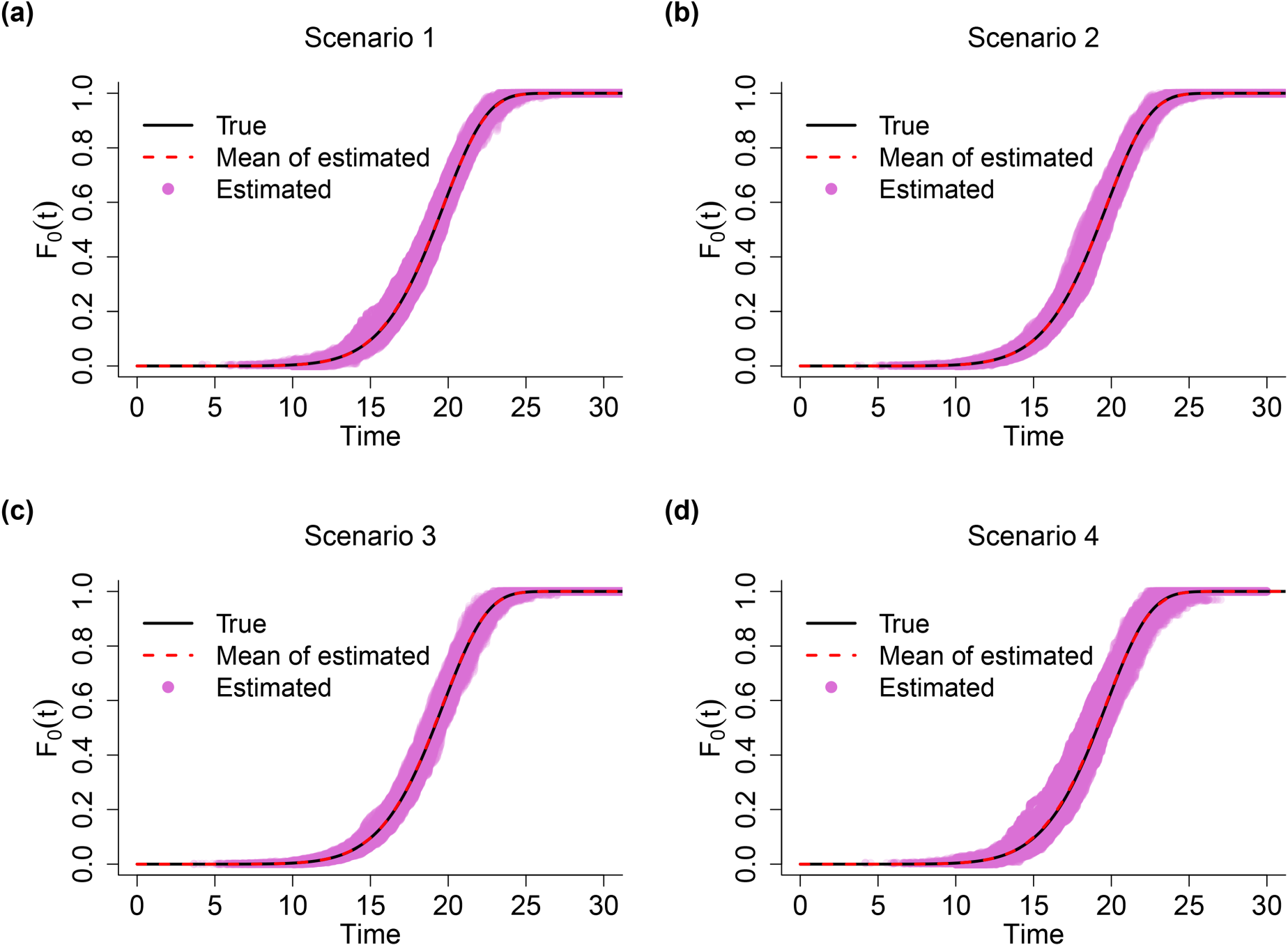
In addition to the good estimation results of JMFHC’s regression parameters shown in Table 1, the estimation of non-parametric $F_0(t)$ performed well and is presented in Figure 2. Under each of four scenarios, we can see that the mean curve of estimated $F_0(t)$ overlaps with the true curve of $F_0(t)$ , and the estimated values of $F_0(t)$ from all runs are well clustered around the true curve.

Figure 2.

Comparison of true and estimated $F_0(t)$ functions from the joint model with a flexible-hazards cure model for survival data (JMFHC) under simulation scenarios 1–4. The true $F_0(t)$ was set as $1-\exp \{-(t/20{)}^8\}$ , which is presented by the black curve. Each red shaded curve represents the mean of estimated $F_0(t)$ functions from 500 runs in each scenario. Pink dots are the estimated values of $F_0(t)$ from 500 runs.

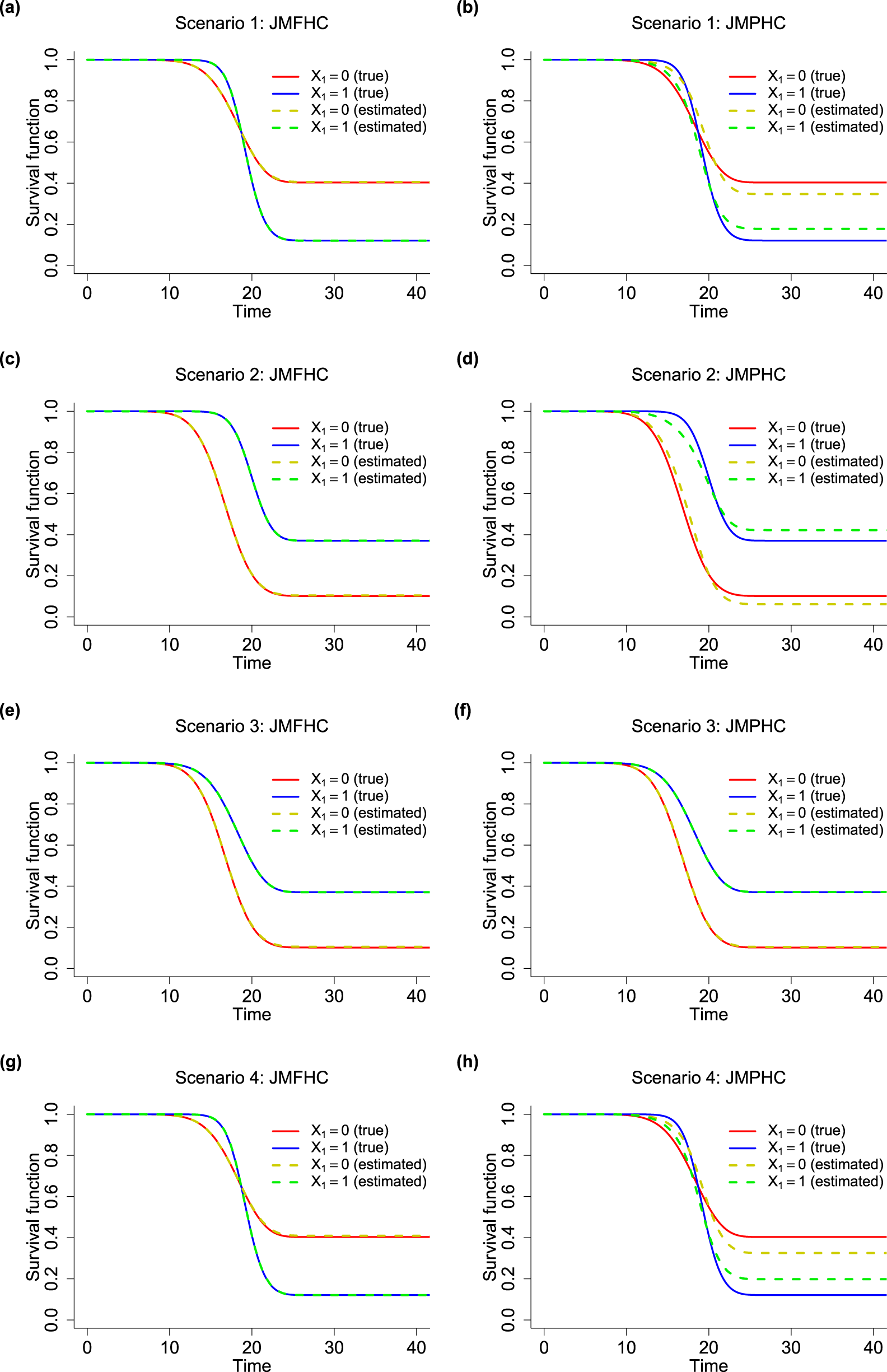
JMFHC easily captured covariates with non-PH structures. In Figure 3, we compared the means of estimated survival functions by $X_1$ from JMFHC and JMPHC with the true survival functions under four scenarios to evaluate the performance of the two models. The estimated survival functions by $X_1$ in each run were the means of survival functions by $X_1$ computed with 1000 randomly generated pairs of random effects given the estimated parameter estimates and $F_0(t)$ from that run. Under scenario 1, the true survival functions by $X_1$ had a clear crossing shown in Figures 3(a) and (b). Subjects with $X_1=1$ had larger survival probabilities or lower hazard rates in an early period than those with $X_1=0$ , but they had smaller survival probabilities in the later period, indicating $X_1$ ’s opposite survival directions for short- and long-term effects. Figure 3(a) shows that JMFHC’s estimated survival functions overlap with the true functions under scenario 1, but JMPHC’s estimated survival functions in Figure 3(b) cannot capture the crossing. Also, JMPHC forced a constant relative hazard rate between two subgroups, and the two stable plateaus at the right tails of JMPHC’s estimated survival functions were closer than the ones from the true survival functions, revealing that JMPHC underestimated the long-term survival effect of $X_1$ . Two models’ performances under scenario 4 shown in Figures 3(g) and (h) are similar to those under scenario 1. Under scenario 2, the true survival functions by $X_1$ with a non-PH structure do not cross as shown in Figures 3(c) and (d). In Figure 3(c), the survival functions estimated by JMFHC overlap with the true survival functions. The violation of the PH assumption caused JMPHC to have estimated survival functions not close to the true survival functions in Figure 3(d). In this case, JMPHC underestimated $X_1$ ’s short-term effect and overestimated its long-term effect. Under Scenario 3, Figures 3(e) and (f) show that the survival functions estimated by JMFHC and JMPHC match the true survival functions.

Figure 3.

True survival functions (solid curves) and means of estimated survival functions (dashed curves) from (a, c, e, g) the joint model with a flexible-hazards cure model for survival data (JMFHC) and (b, d, f, h) the joint model with a proportional hazards cure model for survival data (JMPHC) by $X_1$ (0 vs 1) under simulation scenarios 1–4.

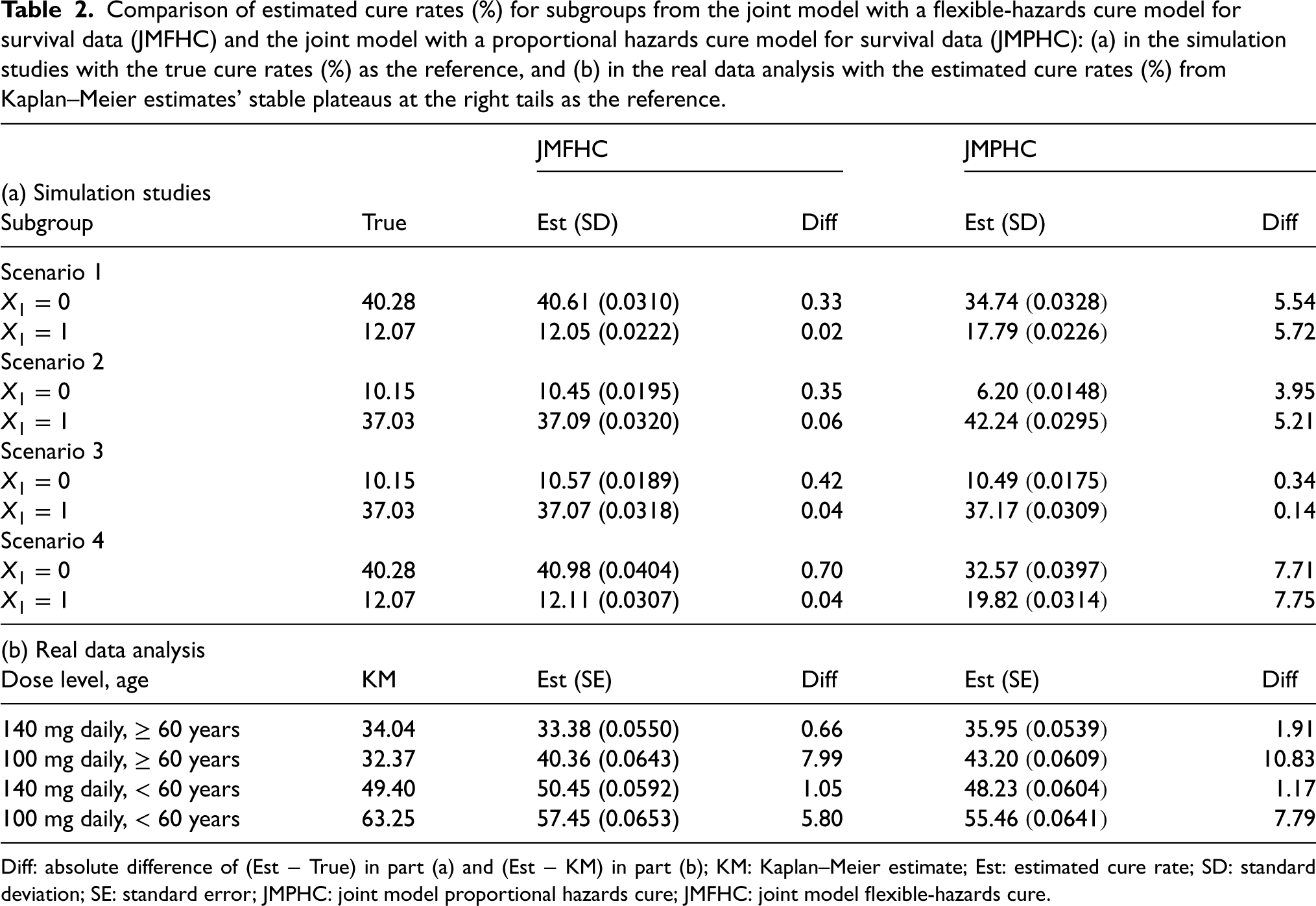
Lastly, JMFHC produced more accurate cure rates than JMPHC. Part (a) of Table 2 shows the true cure rates and the means of estimated cure rates by $X_1$ from JMFHC and JMPHC. The true and estimated cure rates were computed from equation (3) with true and estimated parameter regressions, respectively. JMFHC’s estimated cure rates by $X_1$ were close to the true values in all scenarios. Under scenarios 1, 2, and 4 with a non-PH structure of $X_1$ , the estimated cure rates from JMPHC were biased. JMPHC’s cure rate estimates were close to the true values under scenario 3 satisfying the PH assumption.

Table 2.

Comparison of estimated cure rates (%) for subgroups from the joint model with a flexible-hazards cure model for survival data (JMFHC) and the joint model with a proportional hazards cure model for survival data (JMPHC): (a) in the simulation studies with the true cure rates (%) as the reference, and (b) in the real data analysis with the estimated cure rates (%) from Kaplan–Meier estimates’ stable plateaus at the right tails as the reference.

		JMFHC		JMPHC
(a) Simulation studies
Subgroup	True	Est (SD)	Diff	Est (SD)	Diff
Scenario 1
$X_1=0$	40.28	40.61 (0.0310)	0.33	34.74 (0.0328)	5.54
$X_1=1$	12.07	12.05 (0.0222)	0.02	17.79 (0.0226)	5.72
Scenario 2
$X_1=0$	10.15	10.45 (0.0195)	0.35	6.20 (0.0148)	3.95
$X_1=1$	37.03	37.09 (0.0320)	0.06	42.24 (0.0295)	5.21
Scenario 3
$X_1=0$	10.15	10.57 (0.0189)	0.42	10.49 (0.0175)	0.34
$X_1=1$	37.03	37.07 (0.0318)	0.04	37.17 (0.0309)	0.14
Scenario 4
$X_1=0$	40.28	40.98 (0.0404)	0.70	32.57 (0.0397)	7.71
$X_1=1$	12.07	12.11 (0.0307)	0.04	19.82 (0.0314)	7.75
(b) Real data analysis
Dose level, age	KM	Est (SE)	Diff	Est (SE)	Diff
140 mg daily, $\ge$ 60 years	34.04	33.38 (0.0550)	0.66	35.95 (0.0539)	1.91
100 mg daily, $\ge$ 60 years	32.37	40.36 (0.0643)	7.99	43.20 (0.0609)	10.83
140 mg daily, < 60 years	49.40	50.45 (0.0592)	1.05	48.23 (0.0604)	1.17
100 mg daily, < 60 years	63.25	57.45 (0.0653)	5.80	55.46 (0.0641)	7.79

Diff: absolute difference of (Est $-$ True) in part (a) and (Est $-$ KM) in part (b); KM: Kaplan–Meier estimate; Est: estimated cure rate; SD: standard deviation; SE: standard error; JMPHC: joint model proportional hazards cure; JMFHC: joint model flexible-hazards cure.

In summary, JMFHC and JMPHC work well when the PH assumption holds. When the PH assumption is violated, JMFHC can easily accommodate crossing or non-crossing survival functions by allowing different relative hazard rates in both short and long terms, but JMPHC forces the PH assumption on covariates and produces biased estimated cure rates.

To illustrate our R program’s running time of fitting JMFHC and JMPHC, we took one data set under simulation scenario 1 with crossing survival functions as an example. On a laptop computer with an Intel i7-10610U CPU and 16.0GB RAM, it took JMFHC and JMPHC about 3.9 and 2.5 hours, respectively, to obtain the point estimation. The 500 replicates of simulations with four scenarios were run on the high-performance computing cluster. The running time of jackknife for standard error estimation in one dataset was around 7 hours by using a job array on the high-performance computing cluster.

5. Real data analysis

We compared the results of JMFHC and JMPHC applied to the CML study with 566 patients. This dose optimization study aimed to investigate dasatinib’s optimization of dose level (100 or 140 mg in total per day) and schedule (once or twice daily) for patients with chronic-phase CML who had experienced imatinib resistance or intolerance. Since the schedule of dose taking did not affect the efficacy of dasatinib significantly, ³⁷ we focused our analysis on the effect of dose level [100 mg daily ( $n=269$ ), 140 mg daily ( $n=253$ )] with the disease progression as the event of interest. Besides dose level, the data contains age group (< or $\ge 60$ years) as another clinically significant baseline variable. The censoring rate in this study was 58.0%.

In an LM submodel, the logarithms of the BCR-ABL expression levels were assumed to be associated with the logarithms of measurement time points as fixed and random effects, and dose group and age group as the fixed effects. Figure 1(a) shows the overall trajectory of all patients’ logarithms of BCR-ABL expression gene levels over logarithms of measurement times in years, which presents a roughly linear relationship. The relationship between the logarithms of BCR-ABL expression gene levels and the measurement times in the original form is less linear shown in Figure S1 of the Supplemental Material. In an LM model with the logarithms of the measurement time points as the fixed and random effects, the conditional coefficient of determination $R^2$ interpreting as a variance explained by both fixed and random effects is $0.870$ , which is higher than that of the model with the original measurement time points ( $R^2=0.782$ ). Patient $i$ ’s logarithm of observed BCR-ABL expression level at the logarithm of measurement time point $t_{ij}$ , for $i=1,2,\dots ,566$ and $j=1,2,\dots ,n_i,$ was modeled as

$$\begin{array}{r}\log \{{\text{bcrabl}}_{ij}(t_{ij})\}={\varphi }_0+{\varphi }_1\log (t_{ij})+{\varphi }_2{\text{Dose140}}_i+{\varphi }_3{\text{Age60}}_i+{\alpha }_{i0}+{\alpha }_{i1}\log (t_{ij})+{ϵ}_{ij}\end{array}$$

(16)

where the vector of random effects ${\mathit{\alpha }}_i=({\alpha }_{i0},{\alpha }_{i1}{)}^{\prime }\sim {\mathcal{N}}_2(\mathbf{0},\mathbf{\Sigma })$ with $\mathbf{\Sigma }$ ’s components of ${\sigma }_1,{\sigma }_2$ , and $\rho$ , and ${\mathit{ϵ}}_{\mathit{i}}\sim {\mathcal{N}}_{n_i}(\mathbf{0},{\sigma }_{ϵ}^2{\mathit{I}}_{{\mathit{n}}_{\mathit{i}}})$ .

In the Cox model with dose level, age group, and baseline BCR-ABL expression as the covariates, dose level and age group were significant. The age group violated the PH assumption significantly ( $p$ -value=0.026) from the Grambsch-Therneau test ⁴² and was set as a short-term covariate in JMFHC’s cure submodel. The long-term covariates in JMFHC and JMPHC were dose [Dose140 (mg daily), 1: 140, 0: 100], age [Age60 (years), 1: $\ge$ 60, 0: < 60], and a shared set of individuals’ random intercepts and slopes obtained from the LM submodel. With the shared set of random effects ${\mathit{\alpha }}_{\mathit{i}},i=1,2,\dots ,566$ , the cure submodel of JMFHC for patient $i$ at survival time $T$ was expressed as

$$\begin{array}{r}\begin{array}{rl}& S^{\text{JMFHC}}(t|{\text{Dose140}}_i,{\text{Age60}}_i,{\alpha }_{i0},{\alpha }_{i1})\\ & =\exp [-\exp ({\beta }_0+{\psi }_1{\text{Dose140}}_i+{\psi }_2{\text{Age60}}_i+{\eta }_1{\alpha }_{i0}+{\eta }_2{\alpha }_{i1})\{F_0(t){\}}^{\exp ({\gamma }_1{\text{Age60}}_i)}]\end{array}\end{array}$$

(17)

In JMPHC’s cure submodel, ${\gamma }_1=0$ . The estimation for JMFHC and JMPHC used the same convergence criteria, maximum number of iterations, and scenario of chains in the AM algorithm mentioned in Section 4.

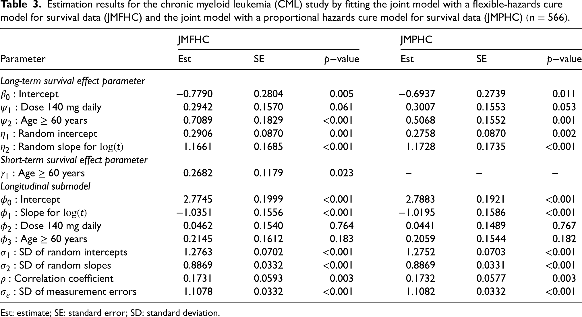
Table 3 presents the estimated regression parameters from JMFHC and JMPHC. In the cure submodels of these two models, dose, age, and individual-specific random effects had the same directions of long-term survival effects and significant effects on PFS at the significance level of 0.05. In JMFHC, age’s short- and long-term parameter estimates indicated that the directions of its short- and long-term effects differed, and patients aged $\ge$ 60 years had significantly better short-term survival ( $p$ -value = 0.023) and worse long-term survival ( $p$ -value $<0.001$ ) than those < 60 years old. Regression parameters in the two models’ longitudinal submodels have similar results.

Table 3.

Estimation results for the chronic myeloid leukemia (CML) study by fitting the joint model with a flexible-hazards cure model for survival data (JMFHC) and the joint model with a proportional hazards cure model for survival data (JMPHC) $(n=566)$ .

	JMFHC			JMPHC
Parameter	Est	SE	$p-$ value	Est	SE	$p-$ value
Long-term survival effect parameter
${\beta }_0:$ Intercept	−0.7790	0.2804	0.005	−0.6937	0.2739	0.011
${\psi }_1:$ Dose 140 mg daily	0.2942	0.1570	0.061	0.3007	0.1553	0.053
${\psi }_2:$ Age $\ge 60$ years	0.7089	0.1829	<0.001	0.5068	0.1552	0.001
${\eta }_1:$ Random intercept	0.2906	0.0870	0.001	0.2758	0.0870	0.002
${\eta }_2:$ Random slope for $\log (t)$	1.1661	0.1685	<0.001	1.1728	0.1735	<0.001
Short-term survival effect parameter
${\gamma }_1:$ Age $\ge 60$ years	0.2682	0.1179	0.023	–	–	–
Longitudinal submodel
${\varphi }_0:$ Intercept	2.7745	0.1999	<0.001	2.7883	0.1921	<0.001
${\varphi }_1:$ Slope for $\log (t)$	−1.0351	0.1556	<0.001	−1.0195	0.1586	<0.001
${\varphi }_2:$ Dose 140 mg daily	0.0462	0.1540	0.764	0.0441	0.1489	0.767
${\varphi }_3:$ Age $\ge 60$ years	0.2145	0.1612	0.183	0.2059	0.1544	0.182
${\sigma }_1:$ SD of random intercepts	1.2763	0.0702	<0.001	1.2752	0.0703	<0.001
${\sigma }_2:$ SD of random slopes	0.8869	0.0332	<0.001	0.8869	0.0331	<0.001
$\rho :$ Correlation coefficient	0.1731	0.0593	0.003	0.1732	0.0577	0.003
${\sigma }_{ϵ}:$ SD of measurement errors	1.1078	0.0332	<0.001	1.1082	0.0332	<0.001

Est: estimate; SE: standard error; SD: standard deviation.

Cure rates estimated by JMFHC were less affected by a covariate’s non-PH structure than those estimated by JMPHC. Part (b) of Table 2 compares the two models’ estimated cure rates for patient subgroups of different dose levels and age groups with those obtained from stable plateaus of the KM estimates at the right tails. Since we did not know the true parameter values for real data analysis and could not obtain the true cure rates of subgroups, we used the estimated cure rates from the KM estimates as surrogate values. For JMFHC and JMPHC, estimated cure rates were computed as shown in equation (3) with estimated regression parameters for subgroups of dose level and age groups. For each subgroup, cure rates estimated by JMPHC deviated from the corresponding KM estimates more than those estimated by JMFHC. In summary, JMFHC outperforms JMPHC when the PH assumption is violated.

6. Discussion

Our proposed joint model, JMFHC, not only incorporates the longitudinal biomarker but also relaxes the PH assumption on covariates. It possesses improved performance compared to a joint model with a widely used cure submodel requiring the PH assumption. An LM-effects submodel is used to model the longitudinal biomarker, and its random effects are shared with the cure submodel. We extend the PHC model into a cure submodel that can flexibly handle covariates’ effect patterns, which is achieved by adding short-term covariates via raising a power on $F_0(t)$ . In our model, estimated by the Lagrange multiplier method, $F_0(t)$ is a non-parametric function with a constraint. Due to the unknown random effects on patients’ longitudinal biomarker measurements, a non-parametric maximum likelihood estimation method incorporating the MCEM algorithm is applied for regression estimation. The jackknife resampling scheme is applied for standard error estimation. Good performance of the proposed model and its estimation method has been demonstrated by the simulation studies. In simulations, the results of our comparison model, JMPHC, show that if the PH assumption is subject to violation, estimated cure rates are biased. Our proposed model handles this situation well and avoids the bias of estimated cure rates. The real data analysis further illustrates that JMFHC can handle covariates’ non-PH structures and estimate the cure rates more accurately.

Our model assumes the same $F_0(t)$ for different covariate groups. This constraint may bias the estimation of $F_0(t)$ and regression parameters in the submodels, which affects the estimation of cure rates. Stratified baseline cumulative hazard functions in JMFHC merit future research to obtain more accurate estimated cure rates. In addition, we could incorporate time-varying variables as fixed variables in the LM-effects submodel. Last, instead of the shared random effects connecting the submodels for longitudinal biomarker values and survival outcomes, the current value of the longitudinal process can be a time-varying covariate in the survival submodel.^48,57 The joint model using an FHC submodel for cure-survival data with the current value of the longitudinal process as a covariate merits future research.

Supplemental Material

sj-pdf-1-smm-10.1177_09622802251320793 - Supplemental material for A new cure model accounting for longitudinal data and flexible patterns of hazard ratios over time

Supplemental material, sj-pdf-1-smm-10.1177_09622802251320793 for A new cure model accounting for longitudinal data and flexible patterns of hazard ratios over time by Can Xie, Xuelin Huang, Ruosha Li, Yu Shen, Nicholas J Short and Kapil N Bhalla in Statistical Methods in Medical Research